
Abstract
Currently, about 60% of the finishing works for freeform parts are done manually, in this paper a parallel kinematic polishing machine (PKPM) with five degrees of freedom (DOFs) and with structural configurations of the type T3R2 (three translations and two rotations) is presented. The PKPM is a variation of the existing METROM Pentapod. The PKPM has a large yaw angle space and, with the aid of an NC rotation table, it can access any given point of the freeform part. A kinematic analysis is developed, an inverse dynamic model based on Kane's equation and the affine projection method is set up in detail, and a real-time and highly efficient inverse dynamic algorithm is developed; the simulation results show that the presented PKPM could achieve an acceleration which is twice that of gravity. A mixed ℋ2/ℋ ∞ control method is presented and investigated in order to track the error control of the inverse dynamic model; the simulation results from different conditions show that the mixed ℋ2/ℋ ∞ control method could achieve an optimal and robust control performance. This work shows that the presented PKPM has a higher dynamic performance than conventional machine tools.
1. Introduction
Parts with freeform surfaces, such as blades, impellers, moulds etc., have been popularly applied in modern industries. According to the statistics, 60% of the finishing works for parts with freeform surfaces are done by hand globally. The manual polishing process is not satisfactory for the rapid development of modern industry due to its instability, unreliability, inefficiency and high cost. High precision and flexibility are the most important avenues to explore for making the whole polishing industry more efficient, stable and reliable. High precision is the basis for the efficient implementation of the finishing process and flexibility ensures the finishing processes are optimized and their stability and reliability are controlled. Therefore, the development of an automatic polishing machine is very important to the manufacturing industry.
Recently, lots of research has focused on the automatic polishing process. An XYZ Desktop NC machine tool was designed by Fusaomi Nagata to polish the PET bottle mould [1]. A 5-DOF polishing machine, consisting of an XYZ desktop NC machine table and a two-axis polishing robot, was developed to carry out the polishing task for freeform surfaces [2,3]. So far, many automatic polishing systems have been developed based on open architectural industrial robots [4,5]; both the dynamic performance and the precision of the industrial robot are quite poor due to its open-chain architecture.
The parallel manipulators are well known for their high speed, high structural rigidity and high precision etc. Parallel kinematic machines based on parallel manipulators begun to be used increasingly as innovative machining equipment over the last ten years, particularly for freeform parts. Much research focusing on PKMs, such as Delta, Tricept and METROM Pentapod, can be found in the literature [6–11]. Y. Hu and B. Li used a robust design method to propose a hybrid kinematic machine with five DOFs based on the structural configuration of a 4PUS-1RPU parallel mechanism; both the kinematic and dynamic performance indices of the proposed mechanism were carried out [12]. H. Huang, B. Li et al. proposed a novel adaptive parallel manipulator with six DOFs and with a large tilting capacity [13]. The manipulator consists of four identical peripheral limbs and one doubly actuated centre limb. Due to the special architecture, the doubly actuated centre limb could have infinite inverse solutions. In every configuration of the end-effector, the manipulator can adapt its centre limb to the position and orientation with the best dexterity. B. Li, X. Yang et al. analysed the inverse kinematics, dexterity and developed a prototype for a proposed 5-DOF hybrid parallel kinematic machine [14]. Y. Li and Q. Xu introduced the passivity-based robust control method into the tracking control of the PKM with parametric uncertainties [15].
The PKM-based polishing system has the characteristics of high flexibility, lower inertia, high stiffness performance and ease of control in the polishing process. The developed polishing system will be one of the most effective ways to achieve the goals with high precision and flexibility. D. Zhang designed a 3-DOF parallel manipulator with a small tilting angle and used an XY table to finish the freeform surface [16]. J. Zhao and M. Yu developed a hybrid polishing kinematics machine tool for freeform surface finishing [17, 18]. Liao Liang et al. developed a dual-purpose compliant tool-head for PKM for polishing and deburring [19].
In robotics technology, inverse dynamics modelling is one of the most important aspects for controlling a robot with high position precision [20, 21]. The classical computed torque is widely used in industrial robots for its easy realization and real-time control, the computed torque method with static gain is applied to the parallel manipulator to obtain the real-time tracking controller [22]. B. Achili et al. used the coupling of sliding modes and multi-layer perception neural networks to control the trajectory tracking of a C5 parallel robot without an inverse dynamic model [23]. H. Abdellatif et al. used a sliding mode to design the six DOFs parallel robot controller [24]. A robust ℋ ∞ method for tracking error control with disturbance is discussed in comparison to common robotic dynamic control [25, 26].
In this paper a parallel kinematic polishing machine with the motion type of T3R2 and a redundant linear motion actuator in the moving platform is proposed, the modelling, and an analysis of the kinematics and the inverse dynamics of the PKPM are investigated in detail.
This paper is organized as follows: the structural scheme of the parallel kinematic polishing machine (PKPM) is presented in section 2; then the kinematic modelling is developed and a dexterous workspace is obtained in section 3; in section 4 the inverse dynamics of the PKPM based on Kane's equation is developed, and the efficient inverse dynamics algorithm based on Kane's method is presented; in section 5 the mixed ℋ2/ℋ ∞ control method is introduced to the PKPM dynamic tracking error control and the performance of the mixed ℋ2/ℋ ∞ control method is discussed using simulations; the last section contains the conclusions.
2. Mechanism scheme
In this paper a mechanism scheme for the PKPM with a structural configuration of 4URHU-1URHR and a redundant translation is presented. The PKPM is shown in Fig. 1(a), from the figure we can see that the presented PKPM is composed of a moving platform, a fixed platform and five kinematic chains which connect the moving platform and the fixed platform. In order to control the polishing force during the polishing process, the linear motion actuator in the moving platform of the PKPM is introduced to carry a spindle with the polishing tool attached. In addition, a numerical control (NC) rotary table is located in the middle of the fixed platform. The spindle with the polishing tool attached is installed on the moving platform.
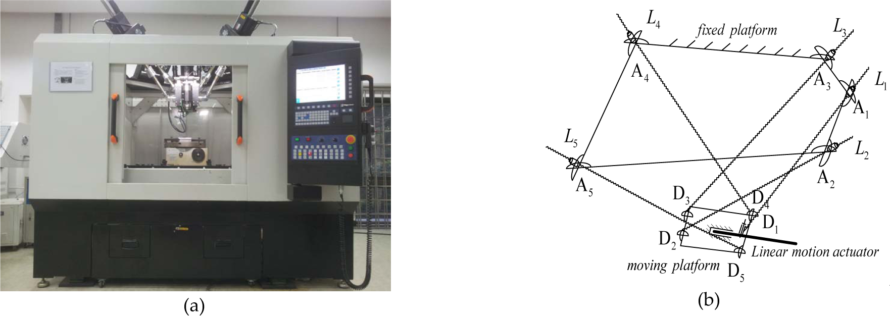
PKPM and the illustrative diagram
The illustrative diagram of the proposed PKPM is shown in Fig. 1(b). The PKM is composed of five kinematic chains, the central kinematic chain L1 consists of a universal joint U, a revolute joint R, a helical joint H and a revolute joint R, the chain can be denoted as URHR and it has five DOFs. The chains of L2, L3, L4 and L5 are four identical 6-DOF kinematic chains denoted by URHU. According to screw theory, the DOF of the moving platform is the same as the central kinematic chain L1, which means that the PKM can provide five DOFs with three translations and two rotations. The actuator installed on the moving platform of the PKM provides the redundant linear motion.
A 3D model of the PKPM can be found in Fig. 2(a). The detailed design of the moving platform is shown in Fig. 2(b), the force sensor and the linear motor are mounted between the moving platform and the spindle, which are used to control the polishing force in the polishing process in order to guarantee that a high surface finish will be obtained. This paper will focus on the modelling and analysis of the dynamic performance of the PKPM in the polishing process.
A famous PKM, the METROM Pentapod, was proposed in 2002 [9]. The PKM structure of the PKPM in this paper is a variation of the METROM Pentapod. The differences between the METROM Pentapod and the PKPM can be described as follows. For the METROM Pentapod, the revolute joints of the kinematic chains connected to the moving platform are in a special configuration, the axes of the revolute joints of the four 6-DOF kinematic chains are collinear with the axis of the spindle, and the axis of revolute joint of the central 5-DOF kinematic chain is perpendicular to the spindle. This special arrangement means that the cutting moment along the axis of the spindle acting on the moving platform will only be carried out by the central kinematic chain, but the other four kinematic chains are not devoted to bearing the cutting moment, so the METROM Pentapod has a relatively low moment-load capability, so the METROM Pentapod is not very suitable for cases where a high cutting moment is carried.

3D model of PKPM and local geometry of the moving platform
The presented PKPM contains two parts: the 5-DOF parallel kinematic mechanism and the linear motion actuator, so the PKPM is the redundant parallel kinematic machine with six driving motors, the structural configuration of the 5-DOF end-effector is T3R2, and the redundant linear translation motion is used to control the polishing force. In order to enlarge the moment-load capability and the stiffness, a variation of the METROM
Pentapod, the PKPM, is developed. The axes of the revolute joints of all the kinematic chains are distributed in three parallel lines, which are not coplanar and are perpendicular to the axis of the spindle, as shown in Fig. 2(b) and Fig. 3. The axis

General notations of the kinematic chain Li
3. Kinematic analysis of the PKPM
3.1 Parametric definitions and coordinate systems
As shown in Fig.3, let P denote a point of a moving platform, it is also the centre point of the revolute joint R at the end of kinematic chain L1, the coordinates of P are xp, yp, zp; ϑ denotes the rotation angle of the moving platform along the axis
According to the definitions, the generalized variables ϑ and φ are not defined in the Cartesian coordinate system, the orientation of the moving platform depends not only on ϑ and φ, but also depends on the position (xp,yp,zp) of the point P in other words, the orientation of the moving platform is coupled with xp, yp, zp, ϑ, φ.
Due to the dynamic equation being set up in the Cartesian coordinate system, it is necessary to transform the velocity and acceleration of the generalized variables into linear/angular velocity and linear/angular acceleration. For convenience of notation, B ij represents the j-th body of the i-th kinematic chain, where Bi1 is the first rotating joint of the universal joint; Bi2 is the stator of the hollow-shaft motor (fixed to the second rotating joint of the universal joint); Bi3 is the rotor of the hollow-shaft motor; Bi4 is the ball-screw; Bi5 is the Cardan-member (moving platform when i=1).
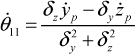
To obtain the velocity and acceleration of the moving platform described in the Cartesian coordinate system by the generalized variables, the intermediate variables θ11, θ12, θ13, θ14, θ15, which denote the joint angles of the central kinematic chain, are introduced to simplify the relationship between the velocity, the acceleration of the moving platform and the generalized variables.
3.2 Kinematic analysis of the central kinematic chain
Note that A1 (xA1, yA1, zA1) denotes the central point of the universal joint of the central kinematic chain; it is a fixed point in relation to the global coordinate system. Let δx=xA1 – xp, δy = yA1 – yp and δz=zA1 – zp′ with the supplementary equations of l = K · (θ13 – ϑ) and

where K= P/2π, P is the screw pitch, l·cosθ12 > 0 ⇒ θ12 ∈ (–90°, 90°) and θ11 ∈ (–90°, 90°) Eq. (1) shows that xp, yp, zp only affect θ11, θ12 and θ13, and θ 11 and θ12 rather than θ13 will decide the orientation of the ball-screw The transformation matrix of the moving platform relative to xp,yp,zp,ϑ and φ can be written as,

where Rs = Rx(θ11) · Ry (θ12) · Rz(ϑ) · Rx(φ); Rx(θ11), Ry(θ12), Rz(ϑ) and Rx(φ) denote the rotation matrices of their corresponding rotation axis, and
For a given vector

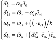
So the angular velocity of the moving platform can be expressed as,

where

The angular acceleration of the moving platform can be written as,

where

According to Eq. (1) the velocity and the acceleration of θ11 and θ12 can be obtained,


where


Combining Eq. (3), Eq. (5) and Eq. (7), the angular velocity of the moving platform can be expressed as,

The linear and angular velocity of the moving platform can be written as,
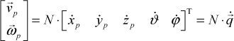
where
The angular acceleration

3.3 Velocity analysis of the kinematic mode
Fig. 4 is a diagram of the kinematic chain L i (i=2, 3, 4 or 5) for the closure vector modelling with the centre kinematic chain L1. The closure equation of the i-th kinematic chain is


Geometric model of the i-th kinematic chain
Let
The first-order derivative of Eq. (12) with respect to t can be written as,

In Eq. (13)

where

Take the inner product with
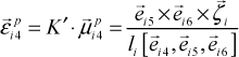
Let
where

where K is a scalar, substituting Eq. (18) to Eq. (17)

Eq. (17) implies

Substituting Eq. (20) to Eq. (19), the angular velocity
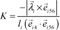
Combining Eq. (18) and Eq. (21), the vector

[·,·,·] denotes a mixed product of three vectors, the angular velocity of the ball-screw in the global coordinate system can be written as,
In order to calculate the angular velocities, the affine projection method is introduced to solve the affine coordinates.
Combining
The angular velocity
3.4 Acceleration analysis of the kinematic model
Take the first-order derivative of Eq. (13) with respect to t, we obtain,

where

where

Take the inner product with

Let

Eq. (29) can be written as,

where

Substituting Eq. (31) to Eq. (30)

Simplifying Eq. (32) we have

The relative angular acceleration
We have the angular acceleration of the ball-screw,

In order to calculate the angular velocities, the affine projection method is used to solve the affine coordinates.
Combining with

The angular acceleration

3.5 Jacobian matrix and the workspace analysis

with
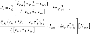
then the kinematic Jacobian matrix can be obtained
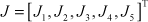
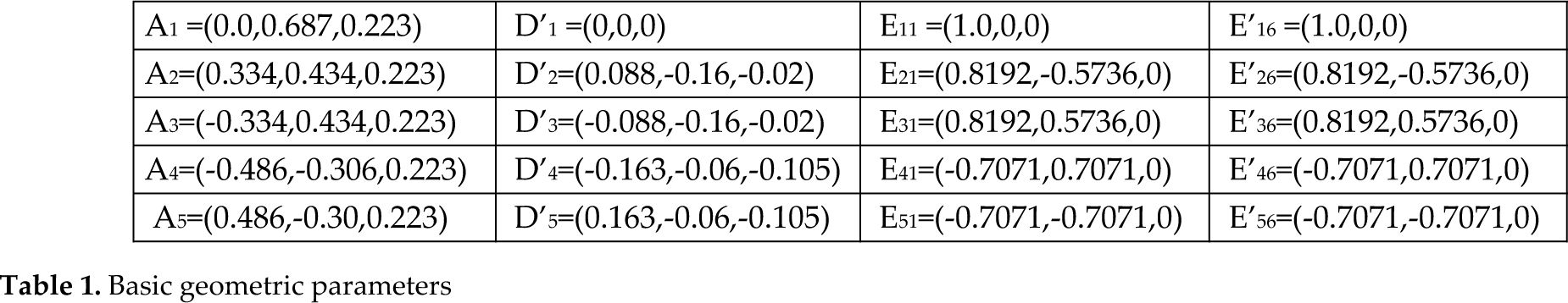
Table 1 contains the basic geometric parameters of the PKPM, D′ i and E′i6 are the local coordinates in the moving platform.
Basic geometric parameters
Let μ(J) denote the condition number of the Jacobian matrix, the dexterous workspace can be searched with the limitation μ(J) <20 by the bound workspace search method, the dexterous workspace of the yaw angle [0°, 90°] and roll angle [-25°, 25°] is shown in Fig. 5, where Fig. 5(a) is the top view of the dexterous workspace and Fig. 5(b) is the oblique view.
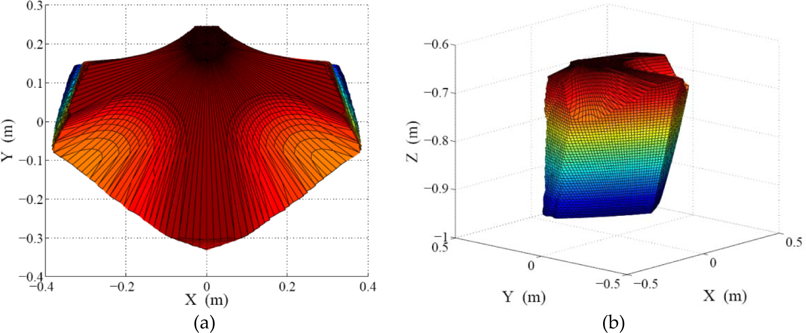
Dexterous workspace of the PKPM
The volume of the dexterous workspace of the PKPM is 0.7 × 0.4 × 0.3 m3, in the dexterous workspace the yaw angle of the moving platform can rotate from 0° to 90°, which means the PKPM is suitable for a large workspace five-axis machine tool.
Fig. 6(a) is the top view of the workspace of the PKPM obtained by fixing the yaw and roll angle of the moving platform to zero, and Fig. 6(b) is the oblique view. As Fig. 6(a)-(b) shows, the volume of the workspace of the PKPM is 1.0 × 1.2 × 0.65 m3, it is larger than that (0.8×0.8×0.5 m3) of the METROM Pentapod.

Workspace of the PKPM with zero yaw and roll angles
4. Inverse dynamics based on Kane's equation
4.1 The Kane's equation method
The Lagrange's equation and the Newton-Euler method are the most common and popular dynamic modelling methods in robotics. They are very efficient and convenient for dynamic systems with low degrees of freedom and few components. The Newton-Euler method requires an analysis of each component of the robot and needs to take the internal forces into account. Finally, it combines the dynamic equations of all the components to obtain the final dynamic equations. So it needs much more work in order to deal with lots of internal forces to obtain the final dynamic equations. The Lagrange's equation based on the energy function does not need to take the internal forces between the components of the robot into account, but it requires that we calculate the second-order derivatives of the Lagrange function. Therefore, the Lagrange's equation is low in efficiency for a system with high DOFs and lots of components.
The Kane's equation method retains the advantages of the vector analysis method and the energy method, and also avoids the drawbacks of Lagrange's equation and the Newton-Euler method. The efficiency of the algorithm based on Kane's method reflects the high efficiency of the modelling and the simple expression of the final dynamic formula. The Kane's equation method does not care about the internal force, so its dynamic modelling is more efficient than the Newton-Euler method. Compared to the Lagrange's equation method, the equations of the dynamic formula of the PKPM based on Kane's equation method are expressed directly in the linear simple matrix form, it can be calculated highly efficiently and can easily be programmed for control.
4.1 Velocity and acceleration of the PKPM components
The mass centre of the body is represented by “C”; each body mass centre of the parallel mechanism is essentially coincident with the geometric centre, so the geometric centre is regarded as the mass centre of the body. As the motion of the component Bi1 is a fixed-point rotation motion through their centres of mass, the linear velocity
Let the distance of component Bi2 deviated from the centre of the universal joint be ρCi2, then the eccentric vector of the mass centre is
The mass centre acceleration of the component Bi3 is

The mass centre of component Bi3 is on the axis of the ball-screw, suppose its eccentric vector is

The mass centre acceleration of the component Bi3 is

Supposing the total length of the ball-screw is L, the mass centre vector of the component Bi4 is
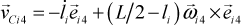
By taking the first-order derivative of Eq. (45) with respect to time t, the mass centre acceleration is

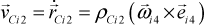
Similarly, the mass centre velocity and acceleration of the component t Bi5 are


In order to obtain the partial velocity of Kane's equation, the angular velocity of each component and the linear velocity of the mass centre relative to the generalized velocity


To simplify the formula expression, we rewrite Eq. (49) and Eq. (50) as Eq. (51):

Similarly, we can combine Eq. (35), Eq. (37), Eq. (42), Eq. (44), Eq. (46) and Eq. (48) into the matrix form:

The coefficient matrices Wij, VCij, Mεij, Maij depend on the generalized variables
4.2 Force analysis
(1) Active force and inertia force of the moving platform
The cutting force and moment and gravity act on the moving platform in the polishing process, so the principal force of the moving platform is,

where
The principal moment acting upon the moving platform can be written as follows,

where
The generalized inertia force

where Ip is the inertia matrix of the moving platform in the global coordinate system;
2) Active force and inertia force of each component
The principal forces and moments acting upon component B ij can be expressed as,


where mij is the mass of B
ij
, M
i
is a driving moment of the hollow-shaft motor in the i-th kinematic chain,
The principal inertia force

where Iij is the inertia matrix of the j-th component in the i-th kinematic chain in the global coordinate system;
Suppose that
4.3 Inverse dynamics of Kane's equation
Variables ẋp, ẏp, żp,


Wij and VCij denote the partial velocity matrix of component B
ij
's linear velocity and angular velocity relative to the generalized variables
Kane's equation shows that all the algebra sums of the generalized driving force

With the partial velocities

where
4.4 Driving torque simulation of inverse dynamics
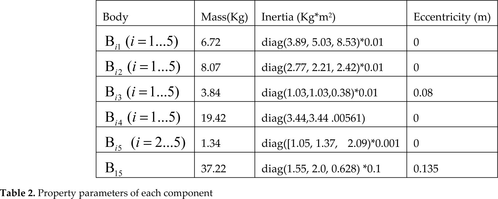
Given the geometric parameters of the PKPM as shown in Table 1, it is easy to calculate the mass and inertia of each component; the geometric and inertia parameters of the ball-screw and the hollow-shaft motor are known, and the inertia of the hollow-shaft motor is 3.8 Kg*m2 and the limit torque is 15 N-m. The property parameters of every component are listed in Table 2.
Property parameters of each component
Suppose the load is just the gravity of the PKPM in the following inverse dynamic torque simulation. Let the moving platform make a circular motion on the plane parallel to the XY plane, and keep both ϑ and φ as zero, the centre of the moving platform is moving in a circular trajectory,
The simulation results of the angular velocities and the driving moments of the motors are shown in Fig. 7
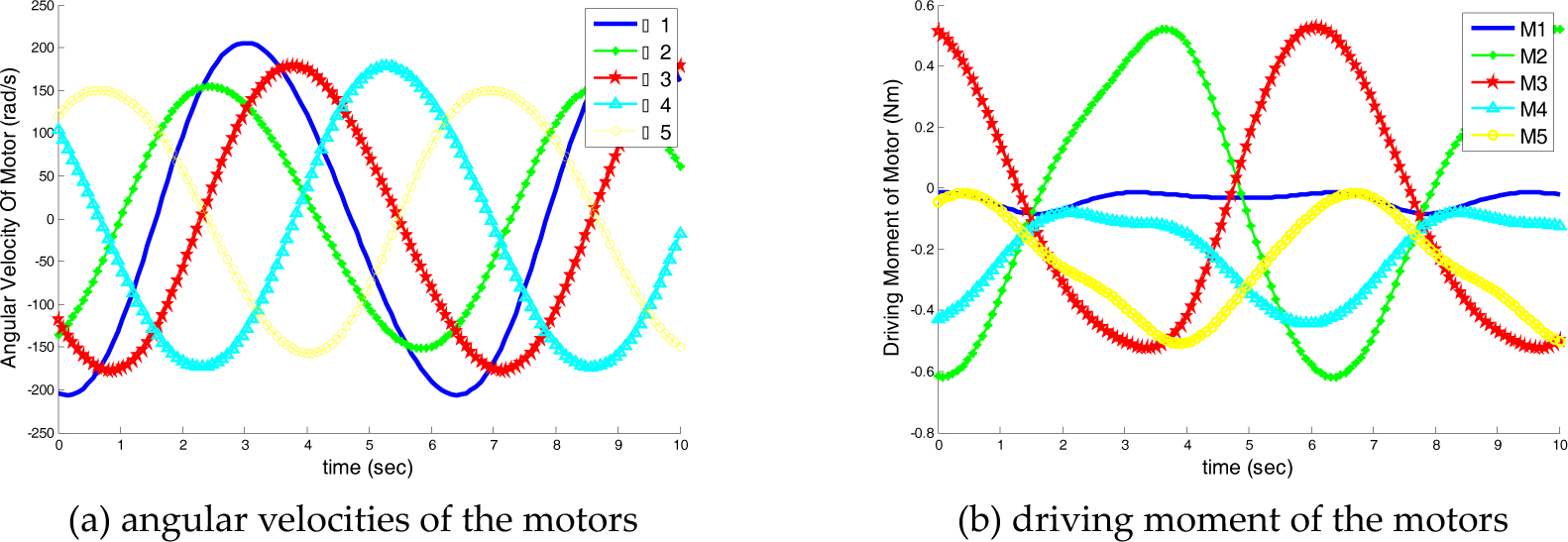
Simulation results (vp =18 m/min, ap = 0.3 m/s2)
The radius and angular velocity of the circular motion is set at rsim = 03m and ωsm = 1 rad/s, so that the linear velocity is rsimωsim = 0.3m/s and the linear acceleration is
Let rsim = 0.0045 m, ωsim = 66.7 rad/s, the polishing feedrate is 18m/min, the acceleration could reach
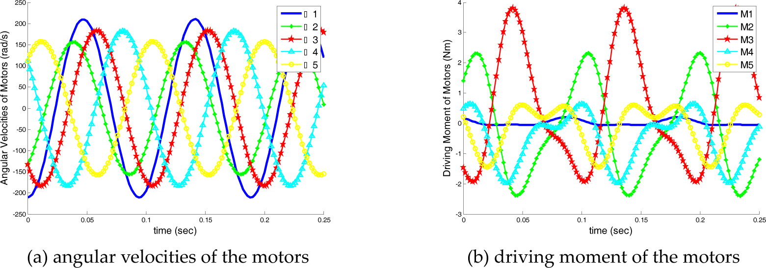
Simulation results (vp =18 m/min, ap =20m/s2)
4. Tracking error control based on the inverse dynamics
4.1 Methods for tracking error control
Currently, there exist many control techniques, such as PID control, computed torque control, slide control, fuzzy control, robust control and so on. The parallel manipulator has a complex structure. From Eq. (62) we know that the dynamic parameters of the parallel mechanism are time-varying.
In the polishing process the trajectory of the polishing tool requires it to be smooth, as the sharp motion and vibration of the polishing tool will deeply affect the polishing precision. As is well known, the slide mode control keeps the robotic motion state around the sliding mode surface, but the switch function of the sliding mode control could make the robot, at a high-frequency, chatter around the sliding mode surface; the chattering would result in a low control accuracy and joint wear occurring quickly.
The friction component
The control gain of the classical PID control method is a constant; hence the classical PID control gain does not satisfy the control of the dynamic parameters in the trajectory motion, so the adaptive control techniques should be introduced to compute the real-time dynamic control gain in order to obtain the optimal tracking error control. The computed torque control is a basic and effective control method in robotic control; with the measurement of the position and velocity of the robot it removes all the nonlinear components of the dynamic equations, so that the nonlinear dynamic control problem is changed into a linear control problem. The control laws of advanced robotic control methods are approximately based on the computed torque control model. In this paper the adapted robust control method with computed torque control is introduced to design the PKPM's trajectory controller.
4.2 Tracking error model and the mixed H2/H∞ control method
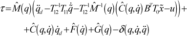
In order to simplify the discussion of designing a motion controller, the inverse dynamic Eq. (62) can be rewritten as,

where τ is used to denote

where M̂ (q), Ĉ (q,q) and Ĝ (q) are the nominal parametric matrices, and ΔM(q), ΔC(q,q̇) and ΔG(q) are the uncertainties. Let τd denote a finite energy exogenous disturbance force, τd is divided into a constant disturbance component τd and a variable disturbance

with

The tracking error of the motion controller decides the motion precision of a robot or machine. For a given motion control object, the best way is to build up its dynamic model with the exact parameters and all the disturbance information, but in the real world there will be some information that cannot be exactly measured or obtained so we need to attenuate the effects of the unknown parameters and the perturbation on the tracking error. For a given trajectory of the moving platform, qd, with its first and second order derivatives, q̇d and

The minimized control action, which includes the minimal applied torque and energy consumption on the motion control, is introduced by R. Johansson [27], considering a more general control action, a state transformation is given by

The applied torque with a variable u for the assignment of the control law is introduced into the robust control design by a minimized control action [26, 27].
Substituting Eq. (69) and Eq. (67) into Eq. (65), the tracking error model based on unknown parameter matrices and external disturbances can be obtained,

where

Let disturbance τd denote the sum of the constant disturbance
For the given positive definite weight matrices Q1, Q2, R1, R2 and an attenuation level γ, the ℋ ∞ tracking error performance for the positive definite matrix Q1f can be expressed as,

The ℋ2 optimal tracking error performance for the positive definite matrix Q2f is written as,

Hence, the mixed ℋ2/ℋ ∞ performance tracking control problem is to find the a pair (u*, w*) which satisfies the minimax problem,


In the mixed ℋ2/ℋ ∞ tracking error control problem, we take R1 = R2 = R to define the same effects of the control variable u(t) in both the ℋ2 and ℋ ∞ performance indices.
The solution of the minimax problem described by Eq. (74) and Eq. (75) turns out to solve a coupled nonlinear time-varying Riccati-like equation, but the nonlinear Riccati-like equations are too difficult to use in engineering. The simple solution for the ℋ2/ℋ ∞ performance tracking error problem is given by introducing some restrictions [26]. For a desired disturbance attenuation level γ, with 0<α<1 and the positive definite weighting matrix of ℋ ∞ , the performance index can be written as,
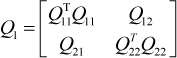
where Q22 = q22I and


Hence, the mixed ℋ2/ℋ ∞ optimal applied torque is
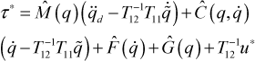
with

Eq. (79) and Eq. (80) can be rewritten in the form of a computed torque,

with mixed ℋ2/ℋ ∞ performance control gain matrices,
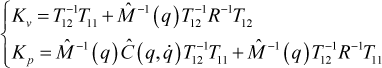
Compared to the classical static gain computed torque control, Eq. (82) shows that the mixed ℋ2/ℋ ∞ performance control has dynamic gain. Hence, the mixed ℋ2/ℋ ∞ performance control is more adaptive than the computed torque control. When the attenuation level γ=∞ is reached, the mixed ℋ2/ℋ ∞ control is degenerated into the ℋ2 optimal control.
4.3 Simulations with four control methods
In this section the computed torque method, the optimal control method, the ℋ ∞ control method and the mixed ℋ2/ℋ ∞ control method for tracking the error control of the PKPM are compared. The classical computed torque control method does not tell us how to obtain the optimal control gain kp and kv, so that we select the control gain kp =200 and kv = 25 for the computed torque control method by experience, and select the attenuation level γ = 0.5 for the ℋ ∞ and the mixed ℋ2/ℋ ∞ method.
The tracking error control focuses on control precision, the attenuation of disturbance, stability and computed driving torque. Four control methods are discussed in this paper. The following simulation is concerned with the disturbance condition. The disturbance is divided into two components, the constant component

Disturbances for simulation
The continuous trajectory command input is shown in Fig. 10. Each trajectory component of the generalized variables of the moving platform is a sinusoidal function relative to the home configuration [0, 0, –0.8, 0, 0]T.

Continuous trajectory command relative to the home position
The simulation results of the continuous trajectory command are shown in Fig. 11(a)-(d). We can see that the optimal control obtains the highest tracking error precision and the lowest one is ℋ ∞ control. This is because the optimal controller is only designed to obtain the high tracking performance and the ℋ ∞ controller is only designed to attenuate the effect of disturbance and unknown parameters. The mixed ℋ2/ℋ ∞ control has a higher tracking error precision than those obtained from computed torque control and ℋ ∞ control.

Simulation results of continuous trajectory command with disturbances
A step function command is used as the simulation's command input,

The position [0, 0, –0.8, 0, 0]T is the origin of the PKPM, the step command trajectory moves the robot to [0, 0, –0.7, 0, 0]T at initial time t0. The step command is shown in Fig. 12.

Step function command
Actually, the driving torque of the hollow-shaft motor is limited by the current passing through the motor, the limited torque of the hollow shaft motor is 15 N·m, hence, we add this torque limit into the dynamic simulation, the simulation results of the step command input are shown in Fig. 13(a)-(d) with the constant disturbance

Simulation results of step trajectory command with disturbances and torque limit
The computed torque controller can track the step trajectory command well, but when the disturbance
The simulation results of the optimal control with driving torque limit show that the tracking error is enlarged to two times that of the step trajectory command input by the optimal control and the dynamic tracking is unstable, so that the optimal control method is not suitable for the step trajectory command.
Because of the disturbance attenuation, the tracking error with the ℋ ∞ control method is insensitive to the external disturbances, but the responsibility of the ℋ ∞ control method is too low to use in tracking the step trajectory command.
From the figure we can see that the tracking error is still smooth when the disturbances
Considering the worst conditions of the step trajectory command with disturbances and driving torque limit, the mixed ℋ2/ℋ ∞ control exhibits both optimal and robust control performance, which means that the mixed ℋ2/ℋ ∞ control method is capable of the attenuation of disturbance with a high tracking error performance.
5. Conclusions
A 5-DOF PKPM with a motion type of T3R2 and a redundant linear motion actuator is developed in this paper, there are two advantages to the structural scheme: one is the large yaw angle workspace which is suitable for polishing parts with freeform surfaces; the second is that the PKPM could perform constant polishing-force control with the 3D force sensor and linear motion actuator mounted on the moving platform. This paper focuses on the inverse dynamic modelling and tracking error control.
The kinematic analysis was developed and a closure vector method was introduced to express the geometric relations of the PKPM linkages, which could avoid a lot of tedious derivations in formulating the linear velocities and angular velocities. The affine projection method was presented as a means to deal with the angular velocities and the angular accelerations projection problem efficiently, so that the linear velocities and the linear accelerations at the mass centre are obtained. Based on these variables an inverse dynamic algorithm based on Kane's equation is developed: it is highly efficient and works in real-time to obtain the driving control torque of the motors. The inverse dynamic driving torque simulation results show that the parallel kinematic machine can work at high speeds and high acceleration. The presented PKPM can achieve an acceleration two times that of gravity, while the conventional machine tool can only achieve an acceleration of one time greater than gravity.
The mixed ℋ2/ℋ ∞ control approach is introduced for PKPM tracking error control. The simulation results from comparing the computed torque method, the optimal control and the ℋ ∞ control method, show that the mixed ℋ2/ℋ ∞ control method with dynamic control gain has a high tracking precision performance and attenuation of disturbances, and a high control performance can also be obtained even under the worst conditions.
Footnotes
6. Acknowledgements
The work is supported by the National Natural Science Foundation of China (Grant No. 51175105); it is also supported by the Shenzhen Key Lab Scheme (CXB200903090033A).