Sage Journals: Discover world-class research

Abstract

This paper presents an improved modelling method for a water jet-based multi-propeller propulsion system. In our previous work, the modelling experiments were only carried out in 2D planes, whose experimental results had poor agreement when we wanted to control the propulsive forces in 3D space directly. This research extends the 2D modelling described in the authors' previous work into 3D space. By doing this, the model could include 3D space information, which is more useful than that of 2D space. The effective propulsive forces and moments in 3D space can be obtained directly by synthesizing the propulsive vectors of propellers. For this purpose, a novel experimental mechanism was developed to achieve the proposed 3D modelling. This mechanism was designed with the mass distribution centred for the robot. By installing a six-axis load-cell sensor at the equivalent mass centre, we obtained the direct propulsive effect of the system for the robot. Also, in this paper, the orientation surface and propulsive surfaces are developed to provide the 3D information of the propulsive system. Experiments for each propeller were first carried out to establish the models. Then, further experiments were carried out with all of the propellers working together to validate the models. Finally, we compared the various experimental results with the simulation data. The utility of this modelling method is discussed at length.

Keywords

Underwater Robots Propulsion System Water Jet Propellers Orientation Surfaces Propulsive Surfaces Surfaces Fitting

1. Introduction

Recently, applications for underwater robots have increased dramatically. They can be found in such diverse areas as mine-clearing operations, feature tracking, cable and pipeline tracking and deep-ocean exploration. The configuration, size, propulsion methods and shape of underwater robots are different for each application. For example, manipulators are necessary for mine-clearing operations. If a robot is used for underwater applications, a smaller, more flexible design may be desirable for easier entry into small spaces; for high-speed movements underwater, a streamlined shape may be required.

The propulsion system is one of the critical features governing the performance of underwater robots because it controls the device. Propulsion devices can have various designs, such as paddlewheels, poles, magneto-hydrodynamic drives, sails and oars.

Paddlewheel thrusters are the most common propulsion method for underwater robots and vehicles. Usually, there are at least two propellers installed per vehicle: one for horizontal movement and the other for vertical movement. A major disadvantage of paddlewheel propellers is that they disturb the water around the underwater vehicle. Biomimetic underwater robots take their designs from nature [1], [2], [3].

The steering strategy of common underwater robots is to change the rudder angle or use differential propulsive forces for two or more thrusters. Vectored propellers are also used on underwater robots and vehicles.

1.1 Related Work

Underwater robots with different sizes and shapes have been reported. Some small autonomous underwater vehicles (AUVs) have also been described [4],[5]. Most of these underwater robots or vehicles are torpedo-like and have streamlined bodies [6]. However, others robots have adopted quite different shapes [7]. All have employed screw propellers for their propulsion system.

Underwater vehicles with vectored thrusters have been described [8], [9]. Multi-channel Hall-effect thrusters involving vector propulsion and vector composition are known [10], [11]. Vectoring thrusters used on aircrafts are also an example of a vectored propulsion system [12], [13], [14].

1.2 Motivation

A spherical underwater robot that used multiple water jet propellers as its propulsion system has been described previously [15], [16], [17], [18]. We have also modelled a single water jet propeller [19]. In [20], an introduction to the development and evaluation of a spherical underwater robot is provided. In the present work, we designed an experimental dynamic model to study the hydrodynamic characteristics of a single water jet propeller while considering the ambient flow.

In our previous work, we used only one strain gage to measure the propulsive force, limiting the accuracy of the model. Since a single strain gage can only detect force in one direction, we only proposed a 2D (horizontal plane) model [17]. We tried to extend the model to three dimensions by incorporating data from basic motion experiments. However, because of the limitations of the modelling method, the agreement of the experimental and simulation results was poor. The propulsive forces and moments used in the 2D space model were not correct for 3D motion; hence, we needed to improve the methodology to obtain more accurate modelling of the water jet propulsion system. For this paper, we redesigned the experimental system so that the modelling could be done properly in 3D space. In particular, we designed a new experimental apparatus so that the mass distribution of the propulsion system was exactly centred on the robot.

1.3 Outline of the Paper

This paper is structured as follows: Section 1 provides the background to the research described. Section 2 introduces the design of the experimental mechanism as well as the orientation vectors and the surface. We also introduce multiple coordinate systems for the propulsion system. The modelling experiments are described in Section 3, with the modelling results illustrated by propulsive surfaces. Section 4 describes the verification experiments and provides a discussion of the results. Section 5 gives the conclusions for this research.

2. Technical Approaches

We needed to model not only a single water jet propeller but also the performance of the whole propulsion system. Consequently, we carried out the modelling experiments directly in 3D space. First, we measured the position of the centre of mass of the robot and then redesigned the experimental mechanism according to the mass distribution and configuration for three water jet propellers.

2.1 Design of the Experimental Mechanism

We were interested primarily in the propulsive effect when the propulsion system is used on the robot rather than just the characteristics of one water jet propeller. In other words, we wanted our experimental mechanism to have a propulsive effect that was equivalent to that of a real robot. Such a mechanism would help us to develop and improve a real propulsion system without requiring underwater experiments with an entire robot. The new experimental mechanism is shown in Fig. 1.

Figure 1.

Design of the experimental mechanism

For the purpose of measuring the mean resultant force and moment in 3D space, we used a BL six-axis load cell sensor (Fig. 2) that could detect forces and torques in the X, Y, and Z directions simultaneously and in real-time. All the propellers were suspended from the centre of the load cell. The relative position between the load cell and three propellers was the same as the position between the robot's mass centre and its three propellers. In this way, we modelled the propulsion system with its propulsive effect as if it were a real robot.

Figure 2.

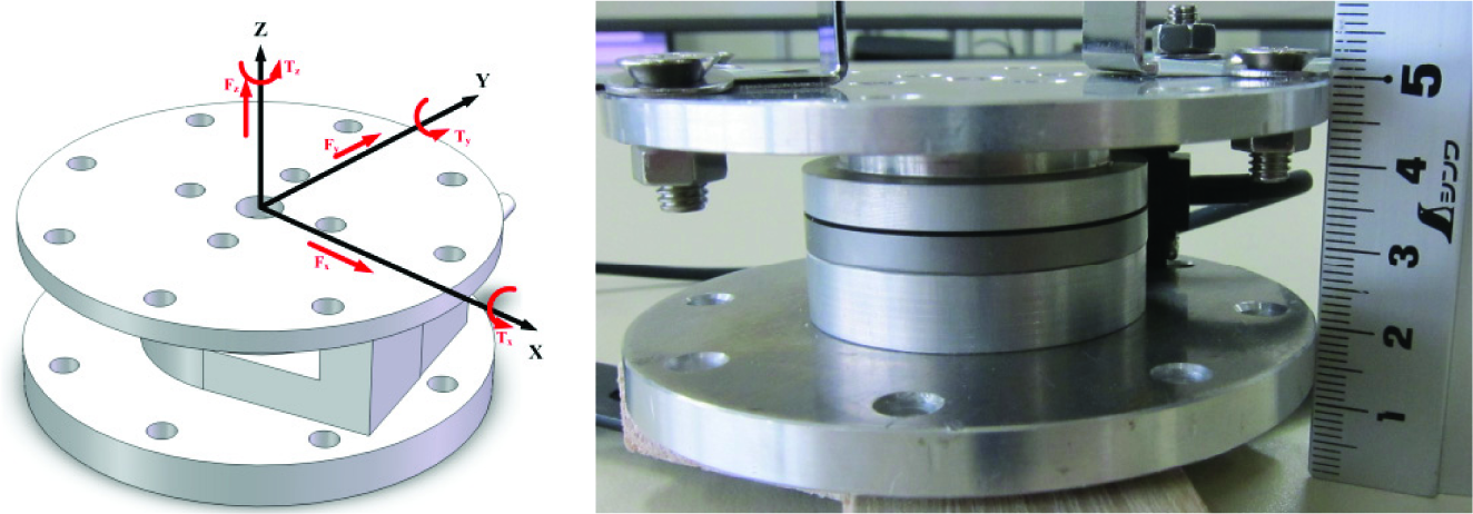
The BL six-axis load cell sensor

2.2 Orientation Vectors and Surface

Orientation vectors and an orientation surface are important in the modelling. We defined a spherical coordinate system for each propeller P: {r, α, β} with an origin Op at the rotational centre of the propeller, as shown in Fig. 3a. With the propeller-fixed coordinates, there were two angles that described the orientation of the nozzle, i.e., the elevation angle α and the azimuth angle β. The front end of the nozzle tracked as a spherical surface So whose centre was at the origin of the propeller-fixed coordinates. The real orientation at each point on the surface was a normal vector that was perpendicular to the surface and passed through the origin of the propeller-fixed coordinate system. Due to the limitation of the robot structure, we only had α∈[−π/3 π/3], β∈e[−π/3 π/3]. The resulting orientation vectors and surface for the water jet propeller are shown in Fig. 3b.

Figure 3.

(a) Propeller-fixed coordinate system; (b) Orientation vectors and surface

The normal vectors of the spherical surface could be used to determine the force vectors and thereby generate the resultant mean propulsive forces. The normal vector space N ∈ ℝ for one water jet propeller denoted in propeller-fixed coordinates was as follows:

n_{p} = (\begin{matrix} \frac{\partial S_{0}}{\partial x} & \frac{\partial S_{0}}{\partial y} & \frac{\partial S_{0}}{\partial z} \end{matrix})

(1)

2.3 Propulsion System Coordinates

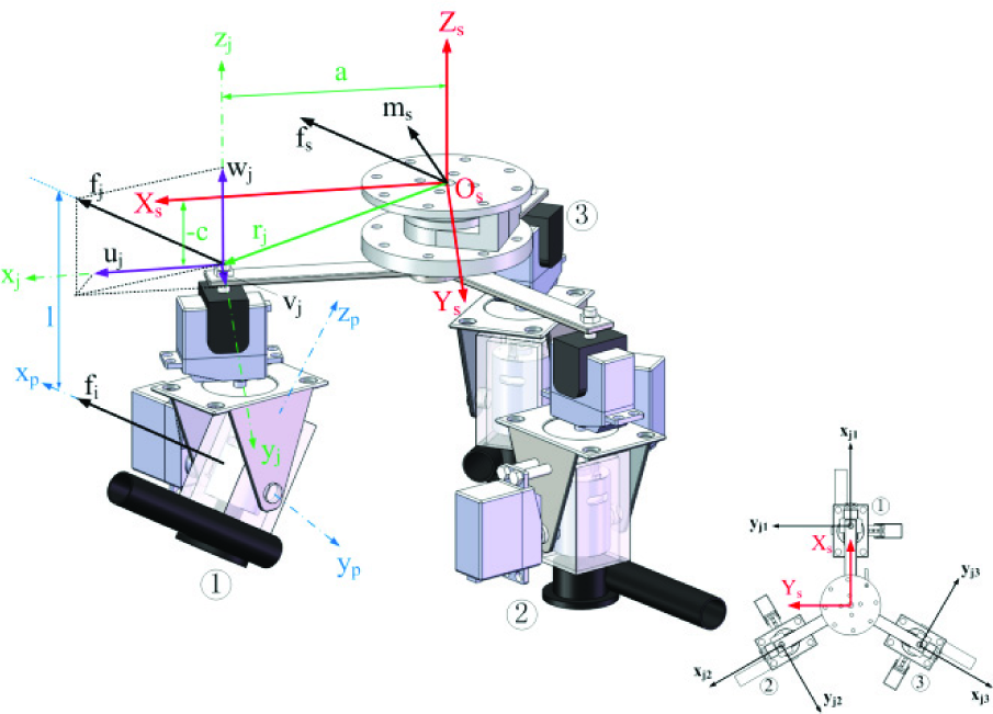
We defined another joint-fixed coordinate J: {xj, yj, zj} whose origin was fixed at the joint screw, as shown in Fig. 4.

Figure 4.

Coordinates of the multiple propellers

Here, f_i is the propeller-fixed coordinate for the i^th propeller; f_j is the equivalent force in joint-fixed coordinates and is the same as f_s, which is in robot-fixed coordinates; l is the position vector of the origin O_p in joint-fixed coordinates; and r_j is the position vector of O_j in robot-fixed coordinates. The equivalent robot-fixed coordinate S: {X, Y, Zs} was located at the top centre of the load cell. We wanted to combine the motions of all three water jet propellers to produce any desired resultant mean force f* and moment T* vectors on the robot.

Each water jet propeller produced a mean force vector f_i in the propeller-fixed coordinate system, which was a 3D space of ℝ³. Therefore, for the i^th propeller in propeller-fixed coordinates, the mean force vector could be given as f_i=(u_i v_i w_i). We also know that, between these three coordinates, the transform rules are:

{\begin{cases} f_{i} = f_{j} = f_{s} \\ T_{i} = T_{j} + f_{j} \times l \\ T_{j} = T_{s} + f_{s} \times r_{j} \end{cases}

(2)

where T is the moment generated by the propellers. r_j can be given as:

r_{1} = [\begin{matrix} a \\ 0 \\ - c \end{matrix}], r_{2} = [\begin{matrix} - \frac{a}{2} \\ \frac{\sqrt{3}}{2} a \\ - c \end{matrix}], r_{3} = [\begin{matrix} - \frac{a}{2} \\ - \frac{\sqrt{3}}{2} a \\ - c \end{matrix}]

(3)

3. Modelling Experiments and Results

The experiments used different α and β as control inputs to obtain propulsive forces and moments as outputs. These variables were input as propeller-fixed coordinates and the outputs were obtained as robot-fixed coordinates. Therefore, the system was like a black box that included a transformation of coordinates. As a result, each propeller had different coordinate transform information. We needed to carry out modelling experiments for each propeller.

We focused on the combination of different direction angles and, therefore, set the mean force of each propeller as a constant 6.5 N. For the modelling, we carried out experiments to determine the relationship between different α, β and r=[f T] for each propeller. For each propeller, we carried out 81 groups of different experiments, with different combinations of α and β for each propeller:

α, ​ β \in [\begin{matrix} - π ∕ 3 & - π ∕ 4 & - π ∕ 6 & - π ∕ 12 & 0 & π ∕ 12 & π ∕ 6 & π ∕ 4 & π ∕ 3 \end{matrix}] .

For each value of α and β was varied from -π / 3 to π/3.

The output forces and moments were functions of α and β. Therefore, the propulsive surfaces were used to describe the relationship between the input direction angles and the propulsive forces and moments. Surface functions were developed to describe these surfaces. The experimental data was first plotted as interpolant surfaces and different surface-fitting methods were evaluated. Finally, we found that a third-order polynomial surface fulfilled our requirement.

The variables f_x, f_y, f_z, T_x, T_y and T_z could be described in the same general form of a third-order polynomial equation, i.e.:

τ (a, b) = \sum_{i = 0}^{3} \sum_{j = 0}^{3} C_{i} ​_{j} a^{i} b^{j}

(4)

where C_ij is the coefficient of the term aⁱb^j, a indicates the value of α, b indicates the value of β. Figs. 5 –7 show the experimental results and fitted surfaces for the propulsive surfaces of propellers 1, 2 and 3, respectively.

Figure 5.

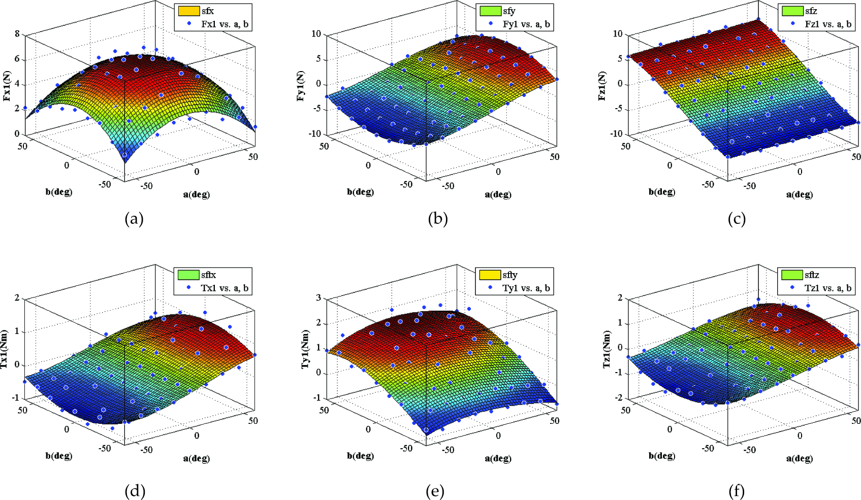
Propulsive surfaces for propeller 1. (a), (b) and (c) are the fitted surfaces for forces in the x, y and z directions, respectively; (d), (e) and (f) are the fitted surfaces for moments in the x, y and z directions, respectively.

Figure 6.

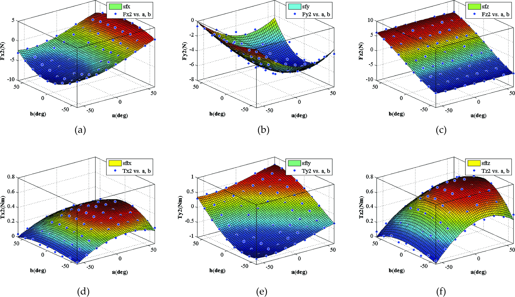
Propulsive surfaces for propeller 2. (a), (b) and (c) are the fitted surfaces for forces in the x, y and z directions, respectively; (d), (e) and (f) are the fitted surfaces for moments in the x, y and z directions, respectively.

Figure 7.

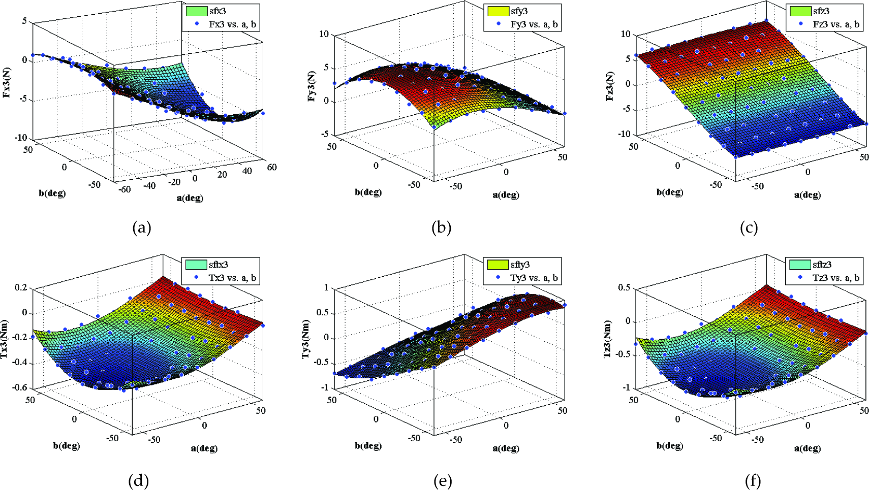
Propulsive surfaces for propeller 3. (a), (b) and (c) are the fitted surfaces for forces in the x, y and z directions, respectively; (d), (e) and (f) are the fitted surfaces for moments in the x, y and z directions, respectively.

It should be noted that the third-order polynomial equation includes the 3D information of coordinate transformation. This means the direct propulsive forces and moments acting on the robot which are expressed in the robot-fixed coordinate can be obtained by simply adjusting the orientation angles in the propeller-fixed coordinate. Therefore, to obtain the effective resultant propulsive force and moment, we can synthesize the propulsive vectors of the propellers in 3D space.

4. Verification and Discussion

4.1 Verification Experiments

Based on the experimental modelling results, we carried out combined experiments using multiple propellers to verify the utility of the model. We first carried out experiments with all the propellers working and at different directional angles, and obtained the effective propulsive forces and moments. Then, we used the modelling results of equation (4) for three propellers to simulate the same running conditions for multiple propellers. Finally, we compared the experimental and simulation results. Because the propulsive forces were actually vectors, the combined experiments required vector synthesis. The force vector could be expressed as:

\begin{array}{l} f (a, b) = f (a, b) n_{p} \\ T (a, b) = T (a, b) n_{v} \end{array}

(5)

where n_p is the orientation vector and n _v is the tangent vector to the orientation surface. We defined α,β∈[−π/3 -π4 -π/6 -π/12 0 π/12 π/6 π/4 π / 3] Figs 8 and 9 show the experimental and simulation results.

Figure 8.

Experimental and simulation results for force verification. (a), (b) and (c) are the experimental results; (d), (e) and (f) are the simulation results.

Figure 9.

Experimental and simulation results for moment verification. (a), (b) and (c) are the experimental results; (d), (e) and (f) are the simulation results.

We know that all the six variables fx, fy, fz, Tx, Ty and Tz have their own model equations which come from the general equation 4. To illustrate the implementation of equation 4, we take the motion in the horizontal plane as an example. In this case, the resultant propulsive force should be in the horizontal plane; meanwhile, the rotation moment should be minimized. Accordingly, the constraint conditions are:

\begin{array}{l} T_{z} = 0 \\ F_{x} = F_{c o n s t 1} \\ F_{y} = F_{c o n s t 2} \end{array}

(6)

where F_const1 and F_const2 are the expected propulsive forces according to the task and the dynamics model. Next, we can solve the equations to get the angles of α and β. We used GPC (Generalized Predictive Control) to control the horizontal motion. In the horizontal plane, we set the control law to change the angles of α and β, and the propulsive forces were set as constant. The control process is that the recognized CARIMA model is built at each sampling time and, accordingly, the control law will adjust to the newly recognized CARIMA model. Moreover, by carrying out the least-squares method, the controller will calculate the necessary value of angles α and β according to the pre-set tracking path in the horizontal plane.

4.2 Discussion

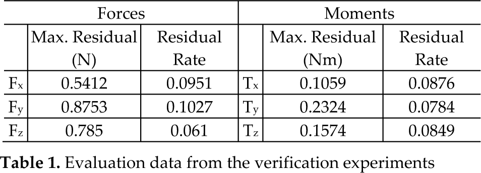
To evaluate the reliability of the verification experiments, we calculated the residuals between the experimental and simulation results. Fig. 10 shows that all the residual plots were evenly distributed around the zero plane, which means that the experimental and simulation results were in good agreement. Table 1 lists the maximum residuals and residual rates for the verification experiments. The maximum residual rate was about 10%, which fulfilled the working requirement for our robot.

Figure 10.

Residuals for verification experiments. (a), (b) and (c) are the residuals for forces; (d), (e) and (f) are the residuals for moments.

Table 1.

Evaluation data from the verification experiments

Forces			Moments
	Max. Residual (N)	Residual Rate		Max. Residual (Nm)	Residual Rate
F_x	0.5412	0.0951	T_x	0.1059	0.0876
F_y	0.8753	0.1027	T_y	0.2324	0.0784
F_z	0.785	0.061	T_z	0.1574	0.0849

5. Conclusions

We have extended the modelling described in our previous work. We considered a transformation of coordinates in the designed the experimental mechanism; thus, the mechanism could be used to find the relationship between the input control signal and output forces/moments. We redesigned the entire experimental device to extend our previous 2D model into 3D space and developed a 3D model for a vectored water jet-based multi-propeller propulsion system.

To develop this model, we first defined the orientation surface in order to describe the orientation of the propeller nozzle; this surface was needed to describe the propulsive vectors. Then, we carried out experiments for each of the propellers. Different combinations of α and β were used, with 81 groups of experiments carried out for each propeller. The experimental data was used to develop a model for propulsive surfaces that included 3D information. Finally, experiments were conducted to verify that the model was applicable when all the propellers were used. These experimental results were in good agreement with the simulation data; their residual rates were acceptable for the implementation conditions defined for our robot.

From the experimental results, the dynamic model of the multiple water jet-based propulsion system was established. According to the experimental data, we employed a third-order polynomial equation which can simply describe the relation of the input signal (orientation angles of the nozzles) and the output (propulsive forces). This equation can be implemented in practical propulsion system control by inversing the equation to get the necessary input orientation angles from the expected propulsive forces.

Footnotes

6. Acknowledgements

This research was supported by the Kagawa University Characteristic Prior Research Fund 2011.

References

Menozzi

Leinhos

H. A.

Beal

D. N.

and Bandyopadhyay

P. R.

(2008) Open-Loop Control of a Multifin Biorobotic Rigid Underwater Vehicle. IEEE Journal of Oceanic Engineering, 33(2), 112–116.

Gao

Guo

and Ye

(2011) Motion-control analysis of ICPF-actuated underwater biomimetic microrobots. Int. J. Mechatronics and Automation, 1(2), 79–89.

Pan

Guo

and Okada

(2011) A Novel Hybrid Wireless Microrobot. Int. J. Mechatronics and Automation, 1(1), 60–69.

Allen

Stokey

Austin

Forrester

Goldsborough

Purcell

and von Alt

(2002) REMUS: A small, low cost AUV; system description, field trials and performance results. OCEANS'97. MTS/IEEE Conference Proceedings, 2, 994–1000.

Madhan

Desa

Prabhudesai

Sebastiao

Pascoal

Desa

Mascarenhas

Maurya

Navelkar

Afzulpurkar

(2006) Mechanical design and development aspects of a small AUV-Maya. 7^th IFAC Conference MCMC2006.

Sangekar

Chitre

and Koay

T. B.

(2008) Hardware architecture for a modular autonomous underwater vehicle STARFISH. IEEE OCEANS 2008, 1–8.

Antonelli

and Chiaverini

(2002) Adaptive tracking control of underwater vehicle-manipulator systems. IEEE International Conference on Control Applications, 2, 1089–1093.

Cavallo

Michelini

R. C.

and Filaretov

V. F.

(2004) Conceptual design of an AUV Equipped with a three degrees of freedom vectored thrusters. Journal of Intelligent & Robotic Systems, 39(4), 365–391.

Le Page

Y. G.

and Holappa

K. W.

(2002) Hydrodynamics of an autonomous underwater vehicle equipped with a vectored thrusters. OCEANS2000 MTS/IEEE Conference and Exhibition, 3, 2135–2140.

10.

Duchemin

Lorand

Notarianni

Valentian

and Chesta

(2007) Multi-Channel Hall-Effect Thruster: Mission Application and Architecture Trade-Offs. 30^th International Electric Propulsion Conference, September 17–20.

11.

Le Page

Y. G.

and Holappa

K. W.

(2002) Simulation and control of an autonomous underwater vehicle equipped with a vectored thrusters. OCEANS2000 MTS/IEEE Conference and Exhibition, 3, 2129–2134.

12.

Kowal

H. J.

(2002) Advances in thrust vectoring and the application of flow-control technology. Canadian Aeronautics and Space Journal, 48(2), 145–151.

13.

Beal

B. E.

(2004) Clustering of Hall Effect Thrusters for High-power Electric Propulsion Applications. PhD thesis, The University of Michigan.

14.

Lazic

D. V.

and Ristanovic

M. R.

(2007) Electrohydraulic thrusters vector control of twin rocket engines with position feedback via angular transducers. Control Engineering Practice. 15(5), 583–594.

15.

Guo

Lin

X. C.

Tanaka

and Hata

(2010) Development and control of a vectored water-jet-based spherical underwater vehicle. IEEE International Conference on Information and Automation, 1341–1326.

16.

Guo

Lin

X. C.

and Hata

(2009) A conceptual design of vectored water-jet propulsion system. IEEE International Conference on Mechatronics and Automation, 1190–1195.

17.

Guo

and Lin

X. C.

(2010) Development of a Vectored Water-Jet-Based Spherical Underwater Vehicle, Autonomous Underwater Vehicles, INTECH-Open Access Publisher, ISBN: 978-953-307-432-0, Chapter 1, 3–20.

18.

Lin

X. C.

Guo

(2012) Development of a Spherical Underwater Robot Equipped with Multiple Vectored Water-Jet-Based Thrusters, Journal of Intelligent and Robotic Systems, DOI 10.1007/s10846-012-9651-3 (Online available).

19.

Guo

Lin

X. C.

Tanaka

and Hata

(2010) Modeling of water-jet propeller for underwater vehicles. IEEE International Conference on Automation and Logistics, 92–97.

20.

Lin

X. C.

Guo

Tanaka

and Hata

(2010) Development and Evaluation of a Vectored Water-jet-based Spherical Underwater Vehicle. INFORMATION: An International Interdisciplinary Journal, 13(6), 1985–1998.

3D Modelling of a Vectored Water Jet-Based Multi-Propeller Propulsion System for a Spherical Underwater Robot

Abstract

Keywords

1. Introduction

1.1 Related Work

1.2 Motivation

1.3 Outline of the Paper

2. Technical Approaches

2.1 Design of the Experimental Mechanism

2.2 Orientation Vectors and Surface

2.3 Propulsion System Coordinates

3. Modelling Experiments and Results

4. Verification and Discussion

4.1 Verification Experiments

4.2 Discussion

5. Conclusions

Footnotes

6. Acknowledgements

References