Sage Journals: Discover world-class research

Abstract

The performance of robot manipulators with nonadaptive controllers might degrade significantly due to the open loop unstable system and the effect of some uncertainties on the robot model or environment. A novel Neural Network PID controller (NNP) is proposed in order to improve the system performance and its robustness. The Neural Network (NN) technique is applied to compensate for the effect of the uncertainties of the robot model. With the NN compensator introduced, the system errors and the NN weights with large dispersion are guaranteed to be bounded in the Lyapunov sense. The weights of the NN compensator are adaptively tuned.

The simulation results show the effectiveness of the model validation approach and its efficiency to guarantee a stable and accurate trajectory tracking process in the presence of uncertainties.

Keywords

PID-NN Control Neural Network Compensator Model Free Model Free Adaptive Controller Robot Manipulator

1. Introduction

In highly automated factories, robot manipulators are often employed to increase the production volume and improve the product quality. Model-based control schemes, such as computed-torque control schemes, are widely used among different types of robot control schemes [1],[2]. No matter how well the parameter settings of these model-based controllers are adjusted, the system performance might degrade in the presence of modelled or unmodelled uncertainties. In recent years in order to overcome this problem several approaches have been taken in order to solve the problem of motion tracking in the presence of uncertainties such as adaptive control [1],[3]-[6], sliding-mode control [7],[8], variable structure control (VSC) [9] and most recently robust adaptive control [10]. In sliding-mode control, chattering often occurs in control torque signals. Fuzzy boundary-layers might be employed to reduce the chattering levels with some accuracy trade-offs [11],[12]. Although these techniques improve system performance, they tend to increase the complexity of system dynamics, which requires special attention regarding system stability. The use of neural networks in control systems has increased in recent years, since, as they do not require any detailed knowledge of mathematical and control theories, they reduce the development cost of controllers for complex systems, particularly nonlinear ones.

Neural networks have previously been applied to the control of manipulators [13]-[15]. Owing to the universal approximator property of NN, feedforward NN compensators are sometimes included in model-based controllers [16]-[19]. The success of fuzzy logic has recently encouraged researchers to use it for industrial processes. Nevertheless, the main problem of fuzzy logic is that there is no systematic procedure for the design of a fuzzy controller. Therefore, it is used with a neural network system (neuro-fuzzy algorithm) [20]-[22]. Neural or fuzzy-based sliding-mode controls are also possible. Another choice could be the gradient method [11],[23] which is widely used. However, there is no guarantee of error convergence or system stability when using the gradient method. To overcome these problems, stable-in-the-Lyapunov-sense adaptation algorithms are proposed [24]-[26]. However, in [24], an explicit positive-definite matrix has to be computed as needed in the adaptation algorithms and there is no guarantee of boundedness of the NN weights. In [25]-[28], the boundary problem is solved and the system stability is maintained even in the presence of uncertainties in the desired NN weights. [29]-[30] used fuzzy neural approaches to control the position of the manipulator and [31] proposed a position controller for robot manipulators using a neuro controller with genetic algorithm-based training. The disadvantage of these approaches lies in the use of the selection matrices for the former, whereas the choice of the input to the neural networks depends directly on the desired task, and hence their applications are limited to simple cases, which limits the diversity of the tasks in an imposed constrained motion. In [32], it was shown that neural networks are very effective at compensating for motion/force tracking in the case of a simple planar surface. Recently, [33], [34] proposed a new model free adaptive approach based on feedback linearization in which the measured signal is taken to a specific level with error less than a defined value and then some experimental rules are applied to the system to keep output error near zero. The major advantage of the model free adaptive controller (MFAC) is that there is no need for identification of the system dynamic and only output error is required. Because MFAC and NNP do not rely on a mathematical model of the system and both use adaptive rules for updating their parameters, the results of MFAC and NNP are compared in this study.

The other aim of this paper is to improve controller robustness of the controller by applying a neural network technique in order to compensate for the effect of uncertainties in the robot model. We show that this control strategy is robust with respect to payload and link mass uncertainties.

The rest of the paper is organized as follows: in Section 2, the nonlinear dynamic of the robot manipulator is described. The design procedure of NNP is represented in sections 3. In Section 4, simulation results are illustrated to highlight the advantages of the proposed method. Finally a conclusion is given in Section 5.

2. Nonlinear Model of Articulated Manipulator

The articulated robot manipulator shown in Figure 1 is a so-called “revolute robot manipulator”, “anthropomorphic robot manipulator” or “elbow manipulator”. It is composed of five main components: base, body, shoulder, elbow and forearm. The body or first joint is moved around the vertical axis and its angle is tagged as θ₁. The shoulder or second joint turns around its own horizontal axis and its angle is named θ₂. The last joint or robot elbow is worked as in the previous joint and its angle is called θ₃ [35].

Figure 1.

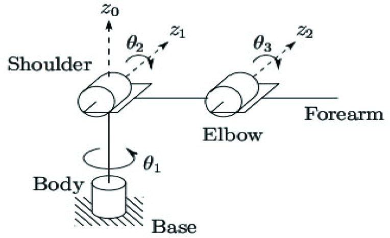
3-DOF articulated robot manipulator scheme [35]

The main objective of control of the robot manipulator is to achieve tracking accuracy in high-speed and high-precision applications. Thus, to have easy control, decrease the computational cost of the controlling process and in order to have got better performance of this system, three motors were employed to make relative torques for every elbow (joint). l₁, l₂ and l₃ are the length of the first, second and third elbow of the robot respectively. The dynamic model of the manipulator is described by the following equation

M (q) \ddot{q} + h (q, \ddot{q}) + G (q) = τ

(1)

where M(q) ∈ R^N×N is a symmetric positively defined inertia matrix, h(q, q̈) ∈ R^N×1 is the vector of Coriolis and centrifugal forces and G(q) ∈ R^N×1 is the gravity forces vector. q∈R^N×1 denotes a generalized position vector in joint-space that in this example q₁, q₂, q₃ are θ₁, θ₂, θ₃ respectively and τ ∈ R^N×1 is a vector of driving torques and finally N is a number of joints. G(q), h(q,q̈), M (q) are described as

\begin{array}{l} M (q) = [\begin{matrix} m_{11} & 0 & 0 \\ 0 & m_{22} & m_{23} \\ 0 & m_{32} & m_{33} \end{matrix}] \\ m_{11} = (m_{4} + m_{3} + 0.25 m_{2}) l_{2}^{2} \cos^{2} (q_{2}) \\ \begin{matrix}  \end{matrix} + (m_{4} + 0.25 m_{3}) l_{3}^{2} \sin^{2} (q_{2} + q_{3}) \\ \begin{matrix}  \end{matrix} + (m_{4} + m_{3}) l_{2} l_{3} \cos (q_{2}) \sin (q_{2} + q_{3}) + 1 \\ m_{22} = (m_{4} + m_{3} + 0.25 m_{2}) l_{2}^{2} + (m_{4} + 0.25 m_{3}) l_{3}^{2} \\ \begin{matrix}  \end{matrix} + (2 m_{4} + m_{3}) l_{2} l_{3} \sin (q_{3}) + 1 \\ m_{23} = (m_{4} + .25 m_{3}) l_{3}^{2} + (m_{4} + .5 m_{3}) l_{2} l_{3} \sin (q_{3}) + 1 \\ m_{32} = m_{23} \\ m_{33} = (m_{4} + 0.25 m_{3}) l_{3}^{2} + 1 \end{array}

(2)

\begin{array}{l} h (q, \ddot{q}) = {[\begin{matrix} h_{1} & h_{2} & h_{3} \end{matrix}]}^{T} \\ h_{1} = {\dot{q}}_{1} {\dot{q}}_{2} [(m_{4} + 0.25 m_{3}) l_{3}^{2} \sin (2 (q_{2} + q_{3}))] \\ - (m_{4} + m_{3} + 0.25 m_{2}) l_{2}^{3} \sin (2 q_{2}) \\ + (m_{4} + m_{3}) l_{2} l_{3} \cos (2 q_{2} + q_{3}) \\ + {\dot{q}}_{1} {\dot{q}}_{3} [(m_{4} + 0.25 m_{3}) l_{3}^{2} \sin (2 (q_{2} + q_{3}))] \\ + (m_{4} + m_{3}) l_{2} l_{3} \cos (q_{2}) \cos (q_{2} + q_{3}) \\ h_{2} = {\dot{q}}_{2} {\dot{q}}_{3} [- (2 m_{4} + m_{3}) l_{2} l_{3} \cos (q_{3})] \\ \begin{matrix}  \end{matrix} \begin{matrix}  \end{matrix} + q_{3}^{2} [- (m_{4} + 0.5 m_{3}) l_{2} l_{3} \cos (q_{3})] \\ \begin{matrix}  \end{matrix} \begin{matrix}  \end{matrix} + 0.5 {\dot{q}}_{1}^{2} [(m_{4} + m_{3} + 0.25 m_{2}) l_{2}^{2} \sin (2 q_{2}) \\ \begin{matrix}  \end{matrix} \begin{matrix}  \end{matrix} + (m_{4} + 0.25 m_{3}) l_{3}^{2} \sin (2 (q_{2} + q_{3}) \\ \begin{matrix}  \end{matrix} \begin{matrix}  \end{matrix} + (m_{4} + 0.5 m_{3}) l_{2} l_{3} \cos (2 q_{2} + q_{3})] \\ h_{3} = - 0.5 {\dot{q}}_{1}^{2} [(m_{4} + 0.25 m_{3}) l_{3}^{2} \sin (2 (q_{2} + q_{3}) \\ \begin{matrix}  \end{matrix} \begin{matrix}  \end{matrix} + (m_{4} + m_{3}) l_{2} l_{3} \cos (q_{2}) \cos (q_{2} + q_{3})] \\ \begin{matrix}  \end{matrix} \begin{matrix}  \end{matrix} - (0.5 {\dot{q}}_{2}^{2} + {\dot{q}}_{2} {\dot{q}}_{3}) (2 m_{4} + m_{3}) l_{2} l_{3} \cos (q_{3}) \end{array}

(3)

G (q) = [\begin{matrix} 0 \\ \begin{array}{l} g [(m_{4} + m_{3} + 0.5 m_{2}) l_{2} \cos (q_{2}) \\ + (m_{4} + 0.5 m_{3}) l_{3} \sin (q_{2} + q_{3})] \end{array} \\ g (m_{4} + 0.5 m_{3}) l_{3} \sin (q_{2} + q_{3}) \end{matrix}]

(4)

Two important issues are investigated in the robot system, “kinematic” and “inverse kinematic”. Robot control actions are executed in the joint coordinates while robot motions are specified in the Cartesian coordinates. Conversion of the position and orientation of a robot manipulator end-effector from Cartesian space to joint space, called the inverse kinematics problem, is an important fundamental issue in calculating the desired joint angles for the robot manipulator. In other words, kinematics relate to the movement of the robot dynamic in terms of joint angles and inverse kinematics relate to the movement of robot in terms of x, y and z (Cartesian coordinates). Their equations are given below.

Kinematic equations:

\begin{array}{l} P_{1} = 1 + \tan^{2} (q_{1}) \\ P_{2} = \tan^{2} (q_{2} + \arctan (\frac{a_{3} \sin (q_{3})}{a_{2} + a_{3} \cos (q_{3})})) \\ P_{3} = a_{3}^{2} + a_{2}^{2} + 2 a_{2} a_{3} \cos (q_{3}) \end{array}

(5)

Inverse kinematic equations:

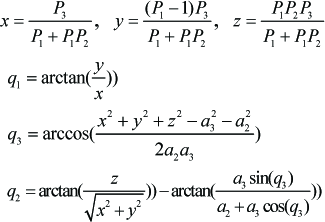
\begin{array}{l} x = \frac{P_{3}}{P_{1} + P_{1} P_{2}}, \begin{matrix}  \end{matrix} y = \frac{(P_{1} - 1) P_{3}}{P_{1} + P_{1} P_{2}}, \begin{matrix}  \end{matrix} z = \frac{P_{1} P_{2} P_{3}}{P_{1} + P_{1} P_{2}} \\ q_{1} = \arctan (\frac{y}{x})) \\ q_{3} = \arccos (\frac{x^{2} + y^{2} + z^{2} - a_{3}^{2} - a_{2}^{2}}{2 a_{2} a_{3}}) \\ q_{2} = \arctan (\frac{z}{\sqrt{x^{2} + y^{2}}})) - \arctan (\frac{a_{3} \sin (q_{3})}{a_{2} + a_{3} \cos (q_{3})})) \end{array}

(6)

where a₃, a₂ are l₃, l₂ respectively and the value of the robot manipulator parameters are shown in Table 1.

Table 1.

Parameters of 3-DOF Robot Manipulator

Parameter	Value
l₁(first link length)	0.15 m
l₂ (second link length)	0.5 m
l₃ (third link length)	0.5 m
m₁ (first link mass)	0.5 kg
m₂ (second link mass)	0.5 kg
m₃ (third link mass)	0.5 kg
m₄ (end-effector – load mass)	3 kg

3. PID with NN Compensator Approach

In this section, the main reason for using the NN in the mathematical framework is illustrated and the effectiveness of the proposed approach in attenuating uncertainties is then proved.

The relation between the joint velocity and the Cartesian space velocity can be expressed as

\dot{X} = J (q) \dot{q}

(7)

Where J(q) represents the n×n Jacobian matrix of the manipulator which is supposed to be nonsingular. By differentiating (7), the Cartesian acceleration term can be expressed as

\ddot{X} = J (q) \ddot{q} + \dot{J} \dot{q}

(8)

Then the equation of robot motion in the joint space can also be represented in Cartesian space coordinates as

\ddot{q} = J {(q)}^{- 1} (\ddot{X} - \dot{J} \dot{q})

(9)

Substituting (9) into (1) yields

τ = A (q) J {(q)}^{- 1} (\ddot{X} - \dot{J} \dot{q}) + C (q, \dot{q}) + G (q)

(10)

The actuator forces are related to the joint torques of the actuators through the Jacobian of the mechanism, consider the following

τ = J^{T} (q) F

(11)

The model of the robot in Cartesian space is thus given by

F = D \ddot{X} + H

(12)

where

\begin{array}{l} D = (J^{T})^{- 1} A J^{- 1}, \\ H = {(J^{T})}^{- 1} [C (\dot{q}, q) + G (q)] - D \dot{J} J^{- 1} \dot{X} \end{array}

(13)

this leads to the following control structure

F = \hat{D} U + \hat{H}

(14)

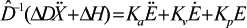
Where U is defined as

U = K_{a} ({\ddot{X}}_{d} - \ddot{X}) + K_{v} ({\dot{X}}_{d} - \dot{X}) + K_{p} (X_{d} - X)

(15)

D̂, Ĥ are the estimates of D and H, respectively; F is the n×1 vector of generalized forces at the end-effector; U is the n×1 vector of the decoupled end-effector; Ka, Kv, and Kp are coefficients of the PID controller. Combining (13), (14) and (15) yields the closed-loop tracking error dynamic equation

{\hat{D}}^{- 1} (Δ D \ddot{X} + Δ H) = K_{a} \ddot{E} + K_{v} \dot{E} + K_{p} E

(16)

where

\begin{array}{c} Δ D = D - \hat{D}, \begin{matrix}  \end{matrix} \begin{matrix} Δ H = H - \hat{H} \end{matrix} \\ \ddot{E} = {\ddot{X}}_{d} - \ddot{X}, \begin{matrix}  \end{matrix} \dot{E} = {\dot{X}}_{d} - \dot{X}, \begin{matrix} E = X_{d} - X \end{matrix} \end{array}

It is should be noted that while the dynamic model is known perfectly, ΔD, ΔH are zeros.

NNP is proposed to achieve disturbance rejection and cancel some drawbacks of uncertainties. The proposed scheme is given in Figure 2. The idea is that the neural network output φ cancels out the uncertainties caused by an inaccurate robot model. The output signal φ of the neural network is added to the control input U whose dimension equals the number of degrees of freedom of the robot manipulator. Therefore, the vector φ is three dimensional. The control law becomes

F = \hat{D} (U + φ) + \hat{H}

(17)

Figure 2.

Anthropomorphic robot manipulator with PID controller and neural network compensator

Combining (8), (10) and (17) yields the corresponding closed-loop system error as

V = K_{a} \ddot{E} + K_{v} \dot{E} + K_{p} E = {\hat{D}}^{- 1} (Δ D \ddot{X} + Δ H) - φ

(18)

In order to drive this error to zero in the presence of the uncertainties, the output of the neural compensator is required to be

φ = {\hat{D}}^{- 1} (Δ D \ddot{X} + Δ H)

(19)

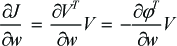
Since the control objective is to generate φ such that V tends to zero, here we propose using V as the error signal for training the neural network. Thus, the ideal value of φ at V=0 is the same as the uncertainties given by (19). Equation (19) is nonlinear and depends on the position, velocity and acceleration of the end-effector. So V is considered as neural network input. The weight updating law minimizes the objective function J, which is a quadratic function of the training signal V

J_{} =_{} \frac{1}{2} V^{T} V

(20)

Differentiating (20) and using (18) yields the gradient of J

{\frac{\partial J}{\partial w}}_{} =_{} \frac{\partial V^{T}}{\partial w} V_{} =_{} - \frac{\partial φ^{T}}{\partial w} V

(21)

The adaptation of the weights is obtained by using the algorithm of retropropagation of the gradient given by the following equation

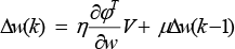
Δ w {(k)}_{} =_{} η \frac{\partial φ^{T}}{\partial w} V +_{} μ Δ w (k - 1)

(22)

Where e˜ is the update rate and μ is the momentum coefficient.

The three layer feedforward neural network structure which is depicted in Figure 3 is used as the compensator. It is composed of linear input layer, output layer and a nonlinear intermediate hidden layer which uses a sigmoid function and is bounded in magnitude between −1 and 1 in accordance with the following equation

f (.) = \frac{1 - \exp (- (.))}{1 + \exp (- (.))}

Figure 3.

Neural Network Compensator

The input is

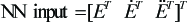
NN  input = {[E^{T} \begin{matrix}  \end{matrix} {\dot{E}}^{T} \begin{matrix}  \end{matrix} {\ddot{E}}^{T}]}^{T}

So this presented algorithm can cancel the effect of modelled or unmodelled uncertainties while it achieves a good tracking performance of the desired trajectory.

4. Simulation Results

For evaluating the performance of the proposed method, two 3-D desired trajectories are considered; in the first the path tracking property of the system is studied by both controllers (NNP and MFAC) and in the second case, uncertainties are enforced on the system while using the NNP controller.

For each trajectory, an asymmetric 3-D curve is produced as the desired path, then the desired angles are obtained using the inverse kinematic equations. The obtained angles are assumed as manipulator target angles. Then desired input is given to the system to be tracked by the articulated robot manipulator. Finally the tracked position which is given by the kinematic equation is acquired using system outputs (actual angels q₁, q₂, q₃). Figure 4 illustrates the system response in Cartesian space gained by NNP and the corresponding 3-D tracking curve can be seen in Figure 5. The same simulation is executed using the MFAC method and the results are shown in Figure 6 and Figure 7. The result clarifies that the NNP can track the desired trajectory more efficiently than MFAC generally. As it is clear from Figure 5, the NNP controller is able to reduce the error in a short time and afterward, the output keeps track of the desired path with an extremely small tracking error. Furthermore, it is seen that the NNP controller is able to keep the error small, even in sharp edges, while with MFAC (Figure 7) there is a large tracking error both at the beginning and after reaching the desired path.

Figure 4.

Simulation results for the 3-DOF articulated robot manipulator in tracking first path using NNP (a) Cartesian space, (b) joint angle

Figure 5.

Simulation results for the 3-DOF articulated robot manipulator in tracking the desired curve using NNP in 3-D Cartesian coordinates

Figure 6.

Simulation results for the 3-DOF articulated robot manipulator using MFAC (a) Cartesian space, (b) joint angle

Figure 7.

Simulation results for the 3-DOF articulated robot manipulator in tracking the desired curve using MFAC in 3-D Cartesian coordinates

In Figure 8 and 9, a 30% payload uncertainty and 10% link mass uncertainties are applied to the system. At the beginning it takes a few seconds for the NN to adapt the parameters to the new condition, but after this transient period it can follow the path very well. Clearly NNP can successfully attenuate the negative effects of the uncertainties due to its adaptive nature.

Figure 8.

Simulation results for the 3-DOF articulated robot manipulator using NNP (a) without uncertainties, (b) with uncertainties

Figure 9.

Actual and desired 3-D curve in Cartesian coordinates using NNP without uncertainties, (b) with uncertainties

5. Conclusion

In this study, we aimed to introduce a new intelligent adaptive controller with a simple structure that can adapt itself to system dynamic uncertainties. Thus, with this procedure we can add an uncertainty rejecting property to PID controllers, which are employed in great numbers by different industries. Simulation results confirm the satisfactory tracking and robustness performances of the proposed controller.

References

Slotine

JJE

(1991) Applied nonlinear controller. Englewood Cliffs, N.J.: Prentice Hall.

Ziauddin

Zalzala

AMS

(1995) Model-based compensation and comparison of neural network controllers for uncertainties of robot arms. IEEE Proceedings: Control Theory and Applications; 142(5):501–507.

Yuan

(1997) Adaptive control of a constrained robot- ensuring zero tracking and zero force errors. IEEE Transactions on Automatic Control; 42(12):1709–1714.

Kamnik

Matko

Bajd

(1998) Application of model reference adaptive control to industrial robot impedance control. Journal of Intelligent & Robotic Systems; 22(2):153–163.

Singh

Popa

(1995) An analysis of some fundamental problems in adaptive control of force and impedance behavior: Theory and experiments, IEEE Transactions on Robotics and Automation; 11(6): 912–921.

Whitcomb

(1997) Adaptive model-based hybrid control of geometrically constrained robot arms, IEEE Transactions on Robotics and Automation 13(1): 105–116.

Belhocine

Hamerlain

Bouyoucef

(1997) Robot control using a sliding mode. Proceedings of the IEEE International Symposium on Intelligent Control, Istanbul, Turkey; pp. 361–366.

Yang

Yamane

Zhang

Zhu

(1998) Sliding mode control of robot manipulator with variable payload. Proceedings of the IEEE International Conference on Intelligent Processing Systems, China; pp. 1312–1316.

Yao

Chan

Wang

(1992) Robust motion and force control of robot manipulators in the presence of environmental constraint uncertainties. Proceedings of the IEEE Conference on Decision and Control, Tucson, AZ, USA, pp. 1875–1880.

10.

Chiu

Lian

(2004) Robust adaptive motion/force tracking design for uncertain constrained robot manipulators. Automatica, 40(12): 2111–2119.

11.

Ertugrul

Kaynak

(1997) Neuro-sliding mode control of robotic manipulators. Proceedings of the Eighth International Conference on Advanced Robotics, Monterey, CA, USA. pp. 951–956.

12.

Lee

(1997) Sliding mode controller with neural network and fuzzy logic. Proceedings of the IEEE International Conference on Neural Networks, USA, 4: 2414–2417.

13.

Choi

Lee

Kim

Kay

(2001) Design and implementation of an adaptive neural-network compensator for control systems, 48(2): 416–423

14.

Wang

Chai

Yang

(2012) Neural-Network-Based Contouring Control for Robotic Manipulators in Operational Space, Doi: 10.1109/TCST.2011.2147316: 1073 – 1080.

15.

Wang

Zhou

(2011) Control of an uncertain nonholonomic mobile manipulator based on the Diagonal Recurrent Neural Network, Control and Decision Conference, Chinese, Doi: 10.1109/CCDC.2011.5968931: 4044–4047.

16.

Fukuda

Shibata

, (1992) Theory and applications of neural network for industrial control systems. IEEE Transactions on Industrial Electronics, 39(6): 472–489.

17.

Ishiguro

Furuhashi

Okuma

Uchikawa

(1992) A neural network compensator for uncertainties of robotics manipulators. IEEE Transactions on Industrial Electronics, 39(6):565–570.

18.

Abdalla

Cai

(1994) Stability analysis of robot manipulators subject to feedforward neural network controllers. Proceedings of the IEEE International Conference on Systems, Man and Cybernetics, USA, 1994; 3: 2588–2593.

19.

Katic

Vukobratovic

(1995) Learning control algorithms for robot contact task using feedforward neural networks. Proceedings of the IEEE International Conference on Intelligent Robots and Systems, Pittsburgh, PA, USA, 3: 522–527.

20.

Selene

Castillo

Aguilar

Castro

(2010) A T-S Fuzzy Logic Controller for biped robot walking based on adaptive network fuzzy inference system, IJCNN: 1–8.

21.

Patricia

Castillo

(2004) Intelligent control of a stepping motor drive using a hybrid neuro-fuzzy approach. Soft Comput. 8(8): 546–555.

22.

Castillo

Melin

(2003) Dynamic systems with a hybrid fuzzy-neural approach. Appl. Soft Comput, 3(4): 363–378.

23.

Jin

(1998) Decentralized adaptive fuzzy control of robot manipulators. IEEE Transactions on Systems, Man, & Cybernetics, Part B: Cybernetics, 28(1):47–57.

24.

Lee

Harris

, (1998) Adaptive neural network control of robotic manipulators. Singapore: World Scientific, 381 p.

25.

Lewis

Jagannathan

Yesildirek

(1999) Neural network control of robot manipulators and nonlinear systems. London: Taylor and Francis, 442 p.

26.

Kim

Lewis

(1998) High-level feedback control with neural networks. Singapore: World Scientific, 216 p.

27.

Lewis

Liu

Yesildirek

(1995) Neural net robot controller with guaranteed tracking performance. IEEE Transactions on Neural Networks; 6(3): 703–715.

28.

Lewis

Yesildirek

Liu

(1996) Multilayer neural-net robot controller with guaranteed tracking performance. IEEE Transactions on Neural Networks 7(2): 388–399.

29.

Kiguchi

Fukuda

(1995) Robot manipulator contact force control application of fuzzy neural network, Proceedings of the IEEE International Conference on Robotics and Automation, Japan, pp. 875–880.

30.

Kiguchi

Fukuda

(1997) Intelligent position/force controller for industrial robot manipulators-application of fuzzy neural networks, IEEE Transactions on Industrial Electronics 44(6): 753–761.

31.

Nakawono

Katagiri

(2003) Force and position control of robot manipulator using neurocontroller with GA based training, Proceedings of IEEE International Symposium on Computational Intelligence in Robotics and Automation, Japan, pp. 1354–1357.

32.

Ferguene

Toumi

(2005) A neural approach to force/position parallel control of robotic manipulators application to the follow-up of trajectory in unknown stiffness environment, Proceedings of the International Conference on Computer Systems and Information Technology, Algeria, pp. 247–251.

33.

Pezeshki

Badamchizadeh

(2010) A New approach for designing of adaptive model free controllers. Journal of Electrical Engineering, Tabriz University, 40(2): 21–36.

34.

Javadi

, and Pezeshki

(2012) A new model-free adaptive controller versus non-linear H∞ controller for levitation of an electromagnetic system. Transactions of the Institute of Measurement and Control, Doi:10.1177/0142331212444664.

35.

Spong

Hutchinson

, and Vidyasagar

(2005) Robot Modeling and Control. John Wiley & Sons, Inc. First Edition, 407 p.

Performance Analysis of a Neuro-PID Controller Applied to a Robot Manipulator

Abstract

Keywords

1. Introduction

2. Nonlinear Model of Articulated Manipulator

3. PID with NN Compensator Approach

4. Simulation Results

5. Conclusion

References