
Abstract
A combined kinematic/torque control law is developed by using a backstepping design approach for a nonholonomic mobile robot with two driving wheels mounted on the same axis to track a reference trajectory. The auxiliary velocity control inputs are designed for the kinematic steering system to make the posture error asymptotically stable. Next, a computed-torque controller is designed such that the mobile robot's velocities converge on the given velocity inputs in an optimal manner by converting the tracking control problem into the regulation problem whereby the uncertainties in the dynamics of mobile robots are considered. The proposed online and forward-in-time policy iteration (PI) algorithm based on approximate dynamic programming (ADP) is used to solve the optimal control problem with unknown internal dynamics by using single neural networks (NNs) to approximate the cost function. Afterwards, the near-optimal control policy can be computed directly according to the cost function, which removes the action network appearing in the ordinary ADP method. The stability of the dynamical extension system is demonstrated using Lyapunov methods. The simulation results are provided to demonstrate the effectiveness of the proposed approach.
1. Introduction
A differentially driven wheeled mobile robot (WMR) is a typical nonholonomic system where the wheels are assumed to roll without slipping [1, 2]. In the mean time, it is also an intrinsically nonlinear system with uncertainties in the dynamic model. The tracking control of such system turns out to be a nontrivial problem due to both its challenging theoretic nature and its practical importance.
Originally, many works [3–6] consider only the kinematic model of the mobile robot, with the assumption that the control signals instantaneously generate the actual velocity control inputs. However, the perfect velocity tracking [7] assumption does not hold in practice.
Controllers based on a full dynamic model [1, 2, 8–10] capture better behaviour because they account for dynamic effects such as mass, friction and inertia, which are neglected by kinematic controllers. Optimization algorithms, such as genetic algorithms (GAs), Ant Colony Optimization (ACO) and Particle Swarm Optimization (PSO), have been used to find the optimal intelligent controller for WMR [11–15]. However, the proposed control scheme only ensures the stability of the closed-loop system and the satisfactory tracking of the output to the given reference signal. There were no optimality criteria which were considered in the control objective. In many cases, it is desirable that the tracking control law not only stabilizes the system but also that it renders optimality based on a pre-defined cost function [16–19].
From a mathematical point of view, the sufficient condition for solving this optimal control problem is the solution to the Hamilton-Jacobi-Bellman (HJB) equation [18, 19]. However, for nonlinear systems, finding a cost function that satisfies the HJB equation is challenging because it requires the solution of a partial differential equation that cannot be solved explicitly. For this reason, considerable efforts have been devoted to developing ADP algorithms [20, 21], including attempts to use, analyse or develop general-purpose methods to find good approximate answers to this optimization problem, using learning or approximation methods to cope with complexity. Actor-critic (AC) architectures [16, 22] have been proposed as models of ADP algorithms since AC methods are amenable to online implementation. Typically, the AC architectures consists of two NNs -an actor NNs and a critic NNs. The actor NNs approximates the optimal control law and generates the control signals while the critic NNs rates the quality of the control signals by the approximation of the cost function.
As part of the optimal control and one of several important new tools for intelligent control, the ADP algorithm presented in this paper does not require preliminary learning. It works online and consists of only one NNs to approximately solve the HJB equation, while the internal dynamics in terms of the velocity tracking errors are considered as unknown difference with AC architectures mentioned above.
The paper is organized as follows. Section 2 provides the kinematic and dynamic model of WMR. The formulation of the adaptive optimal tracking control problem is shown in Section 3 and a unifying design framework is proposed based on a backstepping control approach and nonlinear-optimal control theory. The Lyapunov theory guarantees the stability of the dynamical extension system while considering the error between the cost function and its approximation by using NNs' approximation structures. The convergence proof of the combined control law is presented in Section 4. Section 5 evaluates the control performance of the near-optimal controller by comparing with the initial stabilizing control. Finally, Section 6 gives some concluding remarks.
2. Kinematic and Dynamic Model of the WMR
The WMR as shown in Fig.1 consists of a vehicle with two driving wheels mounted on the same axis and a passive self-adjusted supporting wheel, which carries the mechanical structure. The two driving wheels are independently driven by two actuators (e.g., DC motors). It is assumed that the mobile robot under study is made up of a rigid frame equipped with no deformable wheels and that they are moving on a horizontal plane.
Both wheels have the same radius, denoted by r. The two driving wheels are separated by 2R. The centre of mass of the mobile robot is located at point C. The pose of the robot in the global coordinate frame OXY can be completely specified by three generalized coordinates

System configuration of the WMR
2.1. Kinematic Model
For the WMR system considered here, the pure rolling and non-slipping, nonholonomic condition (1) states that the robot can only move in the direction that is perpendicular to the axis of the driving wheels:

The kinematic constraint (1) can be written as:

The null space of

The vector q̇ has to lie in this null space, therefore:
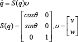
where
2.2. Dynamic Model
Using the Euler-Lagrange equations, the dynamical equations of motion can then be derived as:
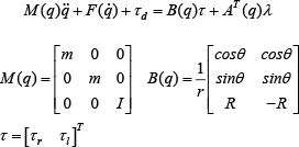
Here, m is the mass, I is the moment of inertia of the robot around its centre of mass,
Next, we differentiate (4) with respect to time, substituting the expression for

3. Control Design
From the perspective of backstepping control, the control design problem of the WMR can be described thus: it generates the desired velocity profiles for the mobile robot to follow a reference trajectory (called motion control) and then the control inputs to the robot (mostly the driving torques/voltages of the motors) are determined to achieve the required velocities that take into account the mass, friction, etc., parameters of the actual cart (called speed control).
3.1. Tracking Control Problem Formulation
In the trajectory tracking task, the mobile robot is required to follow a trajectory generated by a reference robot, prescribed as (7), where it moves at the desired linear and angular velocities,
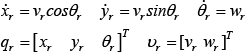
To track a reference trajectory is to find a control law, which makes the real robot follow a given reference moving posture
3.2. Motion Control
The tracking error is expressed relative to the local coordinate frame fixed on the mobile robot as:

and the derivative of the error (8) is:

An auxiliary velocity control input [1] that achieves tracking for (4) is given by:
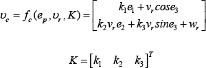
where
since the perfect velocity tracking assumption is unrealistic. Therefore, the actual control inputs to the robot must be considered in order to achieve the required speeds.
3.3. Near-optimal Speed Control
Define the auxiliary velocity tracking error as:

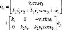
Differentiating (12) and using (6), the mobile robot dynamics may be written in terms of the velocity tracking error as:

where the function
Therefore, a suitable control input for following velocity is given by the computed-torque like control:

where
Using this control input (14) in (13), the closed-loop system becomes:

Eq. (15) can be rewritten as:
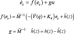
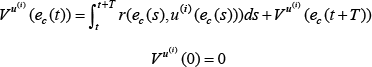
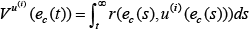
Define the infinite horizon integral cost function as:
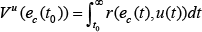
where
Definition 1 Admissible Control
A control
(1)
(2)
Then, an infinitesimal version of (17) is the so-called nonlinear Lyapunov equation:
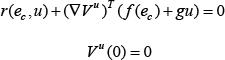
where
The optimal control problem can now be formulated: given the continuous-time system (16), the admissible control set
Defining the Hamiltonian of the problem:

The optimal cost function defined by

Assuming that the minimum on the right hand side of (20) exists and is unique, then the optimal control function for the given problem is:

Inserting this optimal control policy (21) in the Hamiltonian (19), we obtain the formulation of the HJB equation in terms of

In order to find the optimal control solution
In the following, we discuss a new online algorithm based on PI which will adapt to solve the continuous-time (CT) optimal control problem without using any knowledge regarding the system's internal dynamics (i.e., the system function
Proof of the convergence of the algorithm to the optimal control function is provided in next section.
3.3.1. Modified PI Algorithm for Solving the HJB Equation
Instead of trying to solve the HJB equation directly, the PI method starts by evaluating the cost of a given initial policy and then tries to use this information to obtain a new improved control policy.
The modified PI algorithms [19, 23] proposed by the online adaptive critic [16, 21, 24, 25] techniques are built as a two-step iteration, where i denotes the number of iterative steps:
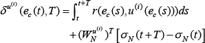
(1) Policy evaluation: solve for the cost function:
(2) Policy improvement: update the control policy using:

Given an initial stabilizing control policy
We solve this iteratively between Eqs. (23) and (24) without making use of any knowledge of the internal dynamics of the system,
3.3.2. Single NNs-based ADP Algorithm for the HJB's Approximate Solution
In order to solve Eq. (22) using the modified PI algorithm proposed previously, we will use a NN to obtain an approximation of the unknown cost function
The cost function

where
Using the NN's approximate description for the cost function
where:
we tune the weights

This amounts to:

Using the inner product notation for the Lévesque integral, (28) can be rewritten as:

According with the properties of the inner product, (29) becomes:

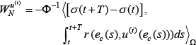
If there exist values of T such that Φ is invertible [17], then we obtain:
From (24), we get the new control policy:

In order to make a difference with (24), we let
Eqs. (31) and (32) are successively solved at each iteration i until convergence.
A general structure for the tracking control system is presented in Figure 2.
4. Convergence Proof
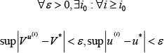
Theorem 1. The policy iterations (23) and (24) converge uniformly to the optimal control problem (17), without using any knowledge of the internal dynamics of the controlled system (16):
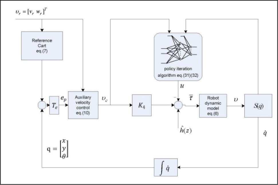
Combined kinematic/torque near the optimal tracking control structure
Proof:
Theorem 1 in [19] shows that
From Eq. (17), we get:
The infinitesimal version of (33) is:

Integrating (34) over the time interval
Thus, assume that the solution of Eq. (18) also satisfies Eq. (23).
Subtracting (18) from (34), we obtain:
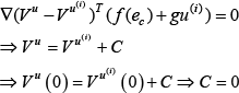
Thus Eq. (23) has a unique solution which is equal to the unique solution of (34).
The algorithm between (34) and (24) is equivalent to the iteration between (23) and (24), which has been proven converge on the solution of the HJB equation [27].
Theorem 2. Given an initial admissible control

Proof:
Due to the Weierstrass Approximation Theorem [2],
where

Let

Due to the fact that the completeness of

Since

Similarly, since
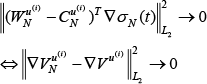

By combining (39)–(41), based on the universal approximation property of multilayer feedforward NNs, when the number of neurons in the hidden layer is sufficiently large, then:

Taking the derivative of

Using (18), we obtain:


Using (24), we obtain

From the result we proved above,
Theorem 3. Given an initial admissible control

Proof:
The results 1, 2 in Theorem 3 follow directly from Theorems 1 and 2.
Establishing a Lyapunov function:

Using (9), we have the expression of

This implies that

From (45) we know that

By assumption

From the above, the exponential stability of the auxiliary velocity tracking error
5. Simulation Results
We would like to implement the near-optimal control scheme presented in Fig. 2 and compare its performance with the initial one to show the effectiveness of the control law developed in this work.
We took the WMR parameters as follows:

The control gains were selected as:

The reference trajectory is generated using the reference model in (7), with

The initial posture for the actual WMR is:
Additionally, we assumed the uncertainties in (16) as:

The weighting matrix Q should be large enough to weigh heavily in the cost function (17). Accordingly, the accumulated states' error could be small and the weighting matrix R should be selected as large if we want to be able to keep the energy consumption as small as possible. For a convenient simulation, we selected
For the NNs, we selected the activation functions with

The initial stabilizing controller was taken as:

Convergence of the NNs' weights
The simulation was conducted using data obtained from the system at every

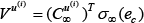
Using (33), we have the expression of the near-optimal controller:

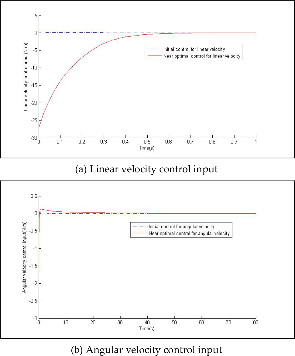
Initial control VS near-optimal control

Velocity tracking error with near-optimal control

Trajectories with initial/ near-optimal control
Fig. 4 shows the initial reinforcement control inputs (46) and the near-optimal reinforcement control inputs (47) for controller (14). We can see the change of the reinforcement control input in controller (14). The velocity tracking error with a near-optimal controller is shown in Fig. 5. The responses with different controllers are shown in Fig. 6 - the tracking error
6. Conclusion
In this paper, we proposed an online PI algorithm based on ADP to solve the optimal control problem with unknown internal dynamics. It uses a single NN to approximate the cost function and then computes the near-optimal control law directly according to the approximation of the cost function. The action networks [22, 25, 28] are no longer needed as an important additional advantage, and the associated iterative training loops are also eliminated. This leads to a notable simplification of the architecture and results in substantial computational savings. Besides this, it also eliminates the NN's approximation error due to the eliminated action networks.
This paper also presents proofs of convergence for the online NNs-based version of the algorithm while taking into account the NN's approximation error. The simulation results support the effectiveness of the online near-optimal controller.