
Abstract
The need to increase security in open or public spaces has in turn given rise to the requirement to monitor these spaces and analyse those images on-site and on-time. At this point, the use of smart cameras – of which the popularity has been increasing – is one step ahead. With sensors and Digital Signal Processors (DSPs), smart cameras generate ad hoc results by analysing the numeric images transmitted from the sensor by means of a variety of image-processing algorithms. Since the images are not transmitted to a distance processing unit but rather are processed inside the camera, it does not necessitate high-bandwidth networks or high processor powered systems; it can instantaneously decide on the required access. Nonetheless, on account of restricted memory, processing power and overall power, image processing algorithms need to be developed and optimized for embedded processors. Among these algorithms, one of the most important is for face detection and recognition. A number of face detection and recognition methods have been proposed recently and many of these methods have been tested on general-purpose processors. In smart cameras – which are real-life applications of such methods – the widest use is on DSPs. In the present study, the Viola-Jones face detection method – which was reported to run faster on PCs – was optimized for DSPs; the face recognition method was combined with the developed sub-region and mask-based DCT (Discrete Cosine Transform). As the employed DSP is a fixed-point processor, the processes were performed with integers insofar as it was possible. To enable face recognition, the image was divided into sub-regions and from each sub-region the robust coefficients against disruptive elements – like face expression, illumination, etc. – were selected as the features. The discrimination of the selected features was enhanced via LDA (Linear Discriminant Analysis) and then employed for recognition. Thanks to its operational convenience, codes that were optimized for a DSP received a functional test after the computer simulation. In these functional tests, the face recognition system attained a 97.4% success rate on the most popular face database: the FRGC.
1. Introduction
Recently and in parallel with the increased importance of security, there has also been a trend towards the use of video cameras in all aspects of life. The rise in video sources has likewise necessitated the birth of smart systems that can automatically process such images and generate results. However, a centre filled with huge numbers of computers not only requires a high amount of image transfer but also increases the related costs. At this point, systems with camera sensors and high-speed embedded system combinations offer a better solution. In addition to being energy efficient, these systems – as they are more compact – offer a better solution for mobile systems, like robotics and traffic [1, 2]. The problem that appears herein concerns the development of appropriate image processing methods for embedded systems.
Increases in the amount of traffic and the human population introduce the requirement to observe and analyse the vehicles and people as well as generate results. At this point, personal rights and freedoms as well as public security emerge as distinct topics. The aim is to monitor and recognize objects. It is the human being which occupies the central position in this subject; in other words, the biometric features of humans matter. Amongst these biometric systems, face recognition -though not achieving high success and unlike others – is distinguished from the other systems since it demands no direct interaction [3]. To illustrate this, physical contact with sensors is necessary to obtain hand biometry and fingerprints. This poses a problem in keeping sensors clean and hygienic. In iris recognition systems – which demand no physical contact – there is an interaction with the sensor [4]. Because there is a dependency on the user, they are not appropriate for a wide range of security applications.
Furthermore, face recognition is a complex process since faces are quite vulnerable to elements such as a change of expression or illumination. Indeed, the changes in the face of the same person can be far greater than the change in the faces of different people.
Face recognition methods can be analysed into two distinctive categories, namely holistic and context-based methods [5]. Holistic approaches extract features by taking the whole face as a high-dimensional signal. Context-based approaches make use of the geometric qualities of the reference points on the face. In other studies, however, methods that divide the face into sub-regions to alleviate disruptive effects like illumination and change of expression have been used [6, 25]. Hence, the advantages of both methods have been combined.
A good number of face recognition methods have been proposed during the past 20 years. These methods have proven to be highly successful in the environments where illumination, expression and pose change are under control, whereas in uncontrolled environments they are not so successful compared with other biometric recognition methods. Therefore, they are still being investigated.
Regardless of the fact that an abundance of methods has been proposed, very few researchers have tested these methods on embedded systems, aside from general-purpose processors (GPU). In one of these methods, Batur et al. [7] designed a face recognition system by employing a C6416 DSP processor with 500MHz. Their research can be analysed in two respects, namely face detection and face recognition. In face detection, in order to minimize the working load, the approach proposed by Kotropoulas and Pitas [8] is employed, stating that “in points where there are sudden, vertical and horizontal floats in profile, there may be boundaries on the face.” With the face recognition method, the Eigenface method has been harnessed and a 93% recognition rate has been achieved for a 10-person database. Actually, the face detection method employed in the current research sought to localize the face on a controlled background, which is why Kotropoulas and Pitas's method was studied. However, this method could not be tested in environments with complex texture information and multiple faces. In face detection, one of the greatest problems concerning processors is the memory and process load which is brought with different-size searches in the image. For instance, in a 640×480 scale image used by Batur, around 1.5 million windows had to be searched to conduct a 20×20 pixel window search with 2 pixel intervals. This is indeed a serious memory and processing problem for even a GPU, let alone for DSPs. In our research, a face search was conducted for 704×576 scale video images and the search was generalized over 2 million windows as well.
Yang and Paindavoine [9] tested for three different embedded systems by using a Radial Basis Function (RBF) neural network-based method for the purpose of localizing and recognizing faces. In the tests conducted for the ORL database, they achieved a 92% success rate for FPGA, an 85% success rate for ZISC and a 98.2% success rate for a DSP. In the study, the power consumptions and speeds of embedded systems were also explored. DSPs – regardless of being the slowest systems – achieved the lowest power consumption and ratio of accuracy. In the test, a 288×352 scale input image was scanned using 40×32 windows through a 2 pixel shift. A total of 10,143 windows were analysed. The number of scanned windows was far smaller than the 2 million windows used in our study.
Günlü [10] harnessed artificial neural networks to conduct face recognition. Unlike other researchers, he tested the training with a DSP. In one particular study, the DSP's effect over the operational speed of cache parameters was analysed. The author achieved an 88% success rate on tests conducted in the ORL database.
Munich et al. [11] created a robot capable of object recognition, navigation and machine-human interaction by employing the Scale Invariant Features Transform (SIFT) method. The Robot 3D could retrieve the images of objects with a camera from different angles, extract 1,000 SIFT features of these objects and then, by using these features, reach recognition. A 600MHz 64-bit RISC processor was employed for the processes. With this processor, a 5 fps speed was obtained for a 208×160 input. In the study, the financial cost of the robot and its applicability for the robotics industry – rather than the algorithm – were analysed.
Theocharides [12] preferred to implement the Viola-Jones method over FPGA. By using the parallel-calculability quality of Haar features in FPGA, he reached a speed of 52 frames per second. In FPGA, he began to search with algorithms alone and used the Open CV library for the training. No information was provided regarding the scales of the images employed for the training and the test.
One of the basic contributions of the current research is that the face detection and recognition algorithm was also adapted for a DSP-based system. To this end, the Viola-Jones method is used for face detection while the block DCT based face recognition method was used for face recognition, with both being analysed at length. An optimization was conducted afterwards in order to determining the memory needs of the method and the stages that would demand the greatest processing power.
Another contribution was made by the sub-region dividing method and the feature selection method, which were applied in the DCT-based face recognition method and which saw a rise in the recognition rate.
Upon dividing the face image into sub-regions, from each sub-region discriminative coefficients in a variety of numbers were selected. By examining the intensity of the coefficients selected from each sub-region, the discriminative value of the related region was computed. It was noticed that the eye and the nose area had further discriminative quality whereas the mouth, cheek and forehead areas were less discriminative. It should be noted that the most discriminative coefficients centred around the eye and nose areas. In comparison with the eye and nose, the discriminative features of the mouth, cheek and forehead areas were smaller.
The algorithm used for embedded platforms was tested for the very first time on the most popular face database FRGC and achieved a recognition rate of over 97%.
In the first part of this paper, information in provided on the previous studies covering embedded systems and their contributions. In the second part, DSP sources and the way in which they are employed in the optimization of vision processing algorithms are explained. In the third part, the Viola-Jones method for face detection and the details of a Discrete Cosine Transform (DCT) algorithm in face extraction are elaborated, and the obtained experimental results are presented. In the fourth part, the algorithm was optimized and run for the DSP and the difficulties experienced and the solution methods are examined. In the conclusion, the obtained findings are reviewed.
2. DSP and optimization
DSPs are distinguished from GPPs (General Purpose Processors) thanks to a set of qualities such as memory management, processing power and architecture. GPPs, in addition to having high processing power and large-scale memories, do not possess highly restrictive forces for image processing algorithms. Furthermore, via the Memory Management Unit in their structure, the memory management operation seen in the algorithms is conducted automatically. The biggest restrictions blocking algorithms in embedded systems are processing power and memory scale. The manual management of memory in the algorithms emerges as one of the obstructing elements. When the signal to be processed is one-dimensional, low performance DSPs can be sufficient, but in image processing with a 2-dimensional signal it is crucial to design memory management and process steps in such a way as to boost the algorithm.
2.1 Embedded Systems
Smart cameras are embedded and system-based. Generally speaking, embedded systems can be divided into subgroups as Reduced Instruction Sets (RISCs), Field Programmable Gate Arrays (FPGAs), Application Specific Integrates Circuits (ASICs) and GPUs [1].
RISC processors mostly integrate the sets of instructions to process in 1 cycle. The most common RISC processor is the ARM processor, which runs in 92% of mobile phones [13].
FPGAs are those units composed of numerous logical gates and they can be programmed via a Hardware Description Language (HDL). Although it is feasible to create complex processors – like FPGAs and DSPs – because of their high price, they are basically employed in applications that demand prototypes or very high processing power.
ASICs contain logical gates prepared to serve a specific application. The most salient feature is that costs are reduced through their manufacture in large quantities.
DSPs are processors which have customized units for signal-processing. They can conduct computation and multiplication which is specifically present in the most innate signal processing methods – like a filter and FFT – and these are the kind of processors whose process performances can be measured via Multiply and Accumulate (MAC). DSPs can process signals as quickly as GPUs, depending on the control of the code-developer over the DSP architecture and algorithm to run. To this end, the codes are mostly written in C++, C and an assembler language. DSPs are generally classified as either Fixed Point or Floating Point. Fixed point DSPs are favoured as they are comparatively faster and cheaper.
GPUs, on the other hand, have basically been customized for graphics processing. The most salient characteristics of these systems is that there are units which can process parallel operations as vectors which enable a faster function of highly complex graphical processes. Despite their similarities with DSPs in certain respects, they consume more power.
Two methods are utilized in developing a program for any particular hardware [1]. In the first method, the program is developed – with no restrictions – for general hardware on a PC. Later, modifications are conducted according to the restrictions of the selected hardware. In the second method, by considering the restrictions of the program hardware and the features of the program, it is developed directly for the selected hardware. In our research we preferred the first method. That is because the program load in the DSP environment, the positioning of the image into the DSP's memory for error debugging and the tools provided for error debugging run much faster in a PC environment.
While developing the algorithm and optimizing for the DSP, a PC-based approach was followed. To this end, the algorithm was run on the DSP to detect the steps that needed to be accelerated. After taking the structure of DSP into account, and by remaking changes to the program on the PC, the required corrections and modifications were implemented.
The greatest restriction for the algorithms is the size of the memory on the DSP. Fast internal RAM is small, while slow external RAMs are comparatively bigger. The developed algorithm was run by transmitting from the external memory to the internal memory. If the data that was to be processed by the algorithm was within the internal memory, it would be processed without any interval, but if the data was within the external memory, the speed of the algorithm would fall substantially. Hence, it becomes necessary to keep the data-to-be-processed inside the internal memory. However, the image characteristics of the data-to-be-processed complicate this procedure and lower the performance of the process.
2.2 DM6437 and ways to increase the process speed
Although the DM6437 has the power to address 4G external memory, in the system we use there is only 128MB external memory at hand. 128kB L2/SRAM, 112kB L1/SRAM are available. The L1/SRAM access time of the processor is 1 process cycle while the L2/SRAM access time is 4 process cycles. The access time to the external memory is above 50 cycles.
The DM6437 has 6 Arithmetical Logical Units (ALU), 2 multipliers and 64 units of 32-bit registers. This processor bears the Very Long Instruction Word (VLIW) attribute. By virtue of this, 8 sets of instructions can be processed concurrently, which enables the compiler to parallelize the instructions.
2.2.1 Single Instruction Multiple Data
One way of accelerating the speed of algorithms is through Single Instruction Multiple Data (SIMD). For instance, regardless of the 32-bit length of registers, in one single register it is possible to run two 16×16-bit or four 8×8-bit processes, which enables the processing of grey level images composed of 8-bit pixels to be four times faster. From the video source, the image is transmitted in the YCbCr format. Since the employed algorithms are colourless, level information alone(Y) was utilized, Cb and Cr – since they carried colour information – were not used in the processes. By eliminating Y from the YCbCr image, grey level image was retrieved. Such 8-bit information is applicable to SIMD processes.
2.2.2 Alignment
Since data buses on DSPs are double-word (64-bit), the alignment of the data in the memory as 64-bit accelerates the speed of the process. However, it is necessary to align video data so as to be applicable to 64-bit accesses. To this end, although the video input is 720×576, for 64-bit alignment, 704×576 part is extracted and processed.
2.2.3 Compiler
There is a discrepancy between the length of the code formed by the compilers and the speed of processing. In order to establish a fast code, the processes need to be parallelized, which in turn increases the length of the code. In our research, we ignored the code length and performed the necessary arrangements to construct the fastest code.
2.2.4 Use of internal memory
It is necessary to integrate the image into the internal memory so as to accelerate the speed of the processor. However, the size of the video image that we processed was far too big to be placed within the internal memory. In this case, it may be useful to process the image by dividing it into sub-regions. Dividing into matching sub-regions as a solution means, on the other hand, making the algorithm even more complex. Besides the designation of the algorithm, the required parameters for each window were first computed and then integrated into the memory at the start in order to allow for a faster operation. Hence, since a considerable amount of memory was separated for that process, it was decided that the process of dividing into sub-regions would offer no solution.
2.2.5 Pipeline
Inside the CPU, instructions are processed in 3 steps, namely fetching, decoding and executing [14]. Because of this, it takes more than one cycle to process every single instruction. However, by means of the pipeline mechanism the processes for each instruction are integrated into one another; in other words, the steps belonging to different instructions are parallel-processed so that in each cycle it becomes possible to process one instruction alone. The formation of a suitable code for the pipeline is concluded during compilation. Software parts that are composed of tiny process groups and multiple amounts of data-to-be-processed are suitable for the software pipeline. It is necessary to inform the compiler in order to achieve this aim. If the compiler fails to detect how many times the cycle will be repeated, it creates a generic code. In that case, since the code does not match the structure of the software pipeline, the process is slowed down. Even though they might consist of simple processes, it may be that not every code can be parallelized; conditioned statements – in particular – are not suitable for this process. Therefore, it becomes necessary to reform the code in order to enable matching.
2.2.6 Making fixed point processes
DSPs are basically designed for fixed point processing. Although DSPs that are capable of floating process have recently been generated, these DSPs are comparatively more costly and slower. However, code development is even more problematic for fixed point processors. In particular, arithmetic overrun and scaling need to be computed attentively.
The algorithm that we developed in the experimental studies was designed as fixed point to make it faster. Nonetheless, in one of the tests we conducted, although face detection provided accurate results for floating processes, it yielded false results for fixed process. The analyses revealed that the processes were not at an adequate level of solution and that the error became even greater during cascade summation. In order to solve this problem, a 64-bit fixed point process was conducted for the problematic process; hence, not only was the dynamic resolution widened but so were the boundaries. Double-word capacity of the DM6437 processor, however, did not increase any loss of speed as much as expected. However, in certain cases the performance that could be gained when a 2×32-bit process was concurrently available was blocked.
One of the most frequently encountered problems in embedded image processing in DSPs is that the processors fail to backup floating point process in terms of the hardware. This problem is a slowing factor in face detection and recognition processes. The algorithms that we employed in the present study are applicable for floating point processes. Fixed point processing is applicable for use with images with preset boundaries. To illustrate this, we conducted an analysis for the integral image used in the Viola-Jones face detector. Every frame of the video image is 576×704 in size. In the worst case, when it is constructed at 255 grey level, the integral value of the extremist pixel is equal to 255×576×704 = 103.403.520, which can be expressed with a 32-bit figure. However, once it is multiplied by the weight value of the window, it will be overrun, and so where there are a significant number of processes it is necessary to have a 64-bit fixed point process.
3. Face Detection and Recognition
The system utilized consists of four sub-modules, namely face detection, feature extraction, feature selection and classification (Figure 1). In the subsequent sections, each sub-unit shall be explained at length.
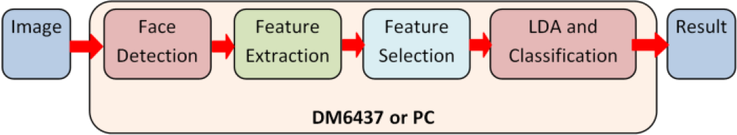
Sub-units of the system utilized in this research
3.1 Face Detection
The detection and alignment of the face to be recognized is directly influential in the success of the recognition method. In face recognition, the information relating to details accelerates the success of recognition for a well-aligned face recognition method, whereas a coarsely-aligned face entry adversely affects the success of recognition.
The Viola-Jones [15, 16] face detection method – due to its speed and high success – is one of the most popular face detection methods [17, 18, 19]. In this method, by shifting a window inside the picture, in every single window the object is searched for via Haar features. The classifier stage is composed of a large number of cascade classifiers with high levels of a False Accept Rate. If a cascade classifier – upon applying every single Haar feature into a window – gains an output above the threshold value, then it applies the next and more complex Haar feature. In Figure 2, the Haar features within the red window have been drawn with blue boundaries. The pixels within the black region are weighted with −1, while the pixels remaining within the white region are weighted with +1. Those Haar features are applied to search windows sequentially, but not all features are applied for all windows. The speed of the method is achieved through cascade classifiers by discarding simple Haar features in the first few searches, namely those regions with the low possibility of being a face. In Figure 3, a histogram for the experimentally acquired stage number where classification was terminated is presented. For a 15×104 window, the search was terminated in the first cascade classifier. 72% of windows ended within the first 2 classifiers and 92% within the first 4 classifiers. Therefore, it became possible to maintain the search with more complex features over 8% of windows with a high potential for bearing face (Figure 3-a). This condition boosted the speed of the method as well. The histogram of the Haar feature number computed for each window is given below. The Haar feature number computed in Figure 3-b decreased exponentially, and a good number of windows were discarded after taking the first features into consideration.

Haar features employed in face detection; inside the red window, the Haar features are indicated with blue boundaries. Those pixels remaining inside the black region are weighted with −1, while those pixels remaining inside the white region are weighted with +1.

(a) In the Viola-Jones method histogram for the stage number where the classification for the searched windows was terminated. 74% of the terminated stages were eliminated in the first 2 stages; 92% were terminated in the first 4 stages. (b) Histogram (logarithmic) for the Haar feature number applied to conduct the search in each window.
Another factor boosting the speed of the method is the “integral pattern” used in computing Haar windows. When the “integral image” is computed for one instant, for each Haar feature computation, 8 summations and 2 multiplications alone prove to be adequate. Additionally, it is not necessary to re-compute the “integral image” to search the face in different scales. The “integral image” concept has been effectively harnessed in the Viola-Jones method during pattern processing. Fast algorithms developed to compute the integral image have also been widely used in embedded applications with low performance levels. By virtue of all of the above, a face search in different scales can be conducted rather quickly.
3.2 Discrete Cosine Transform-based Face Recognition
DCT is quite a popular method in feature extraction by virtue of its data compression capacity, independence of data inputs and fast computation [20, 21, 23]. DCT transforms the signals into the sum of sinuses at varying frequencies. Low frequency DCT coefficients have importance in relation to the expression of the relevant face data. Low frequency DCT coefficients use a great portion of energy. In face recognition problems, these coefficients are transmitted to 1D series through zig-zag scanning; hence, the feature vector is created. Hafed et al. [22] and Ekenel et al. [23] took low frequency DCT coefficients of faces on ORL through low frequency zig-zag scanning and used them for recognition. Notwithstanding the fact that the first coefficients carried a substantial portion of data, these coefficients were comparatively more contingent upon illumination. Thus, in one study [24] it has been suggested the first coefficient should be discarded so that it would be possible to conduct face recognition which is resistant to illumination. As opposed to common practice, it was proposed in the same study to use high frequency coefficients, but this practice requires well-aligned faces since high frequency coefficients are highly sensitive to noise and shift.
Jing et al. [25] divided the DCT coefficients into a set of band regions and after calculating the discriminative power of each band region they utilized the most discriminative regions for the recognition process. In this case, the highest and the lowest band regions were discarded. In the current study, the distinctiveness of every single DCT coefficient was statistically computed so as to be employed in face recognition. However, and as distinct with the previous ones, a definite band region or frequency zone was not discarded intuitively. Each coefficient was selected with respect to their individual or combinational distinctiveness. Details of this issue are provided in the section called the ‘feature selection’. The DCT coefficients obtained from each block were selected in the same way as with the globally obtained DCT coefficients. Nevertheless, since the first coefficients were highly dependent on illumination and change of expression, these coefficients were discarded intuitively. For local 2D DCT, a similar approach was also followed [26].
DCT can be applied over images in two forms: global or local. The DCT applications mentioned so far are global DCT applications. To put it another way, DCT is directly applied to the whole image. By applying 2D DCT on a MxN size image, it is feasible to procure DCT coefficients in a MxN size.
The conversion factors obtained in the global DCT method carry information of the whole image; however, in this case, an attempt was made to code the connection amidst the whole of the points of the image. This, on the other hand, causes a failure of proper-coding amidst the different reference points, particularly on the face. Furthermore, each region on the face is affected at different levels from illumination and changes of expression. In that case, disruptive effects will be influential over all of the DCT coefficients. In order to remedy this failure of global DCT, the use of local DCT has been proposed.
2D DCT transmits spatial signals to frequency regions and hence spatial information cannot be saved. In order to save spatial information in addition to frequency information, the use of local DCT coefficients has been proposed. To this end, by separating face images into blocks, low-frequency DCT coefficients obtained from every block are used as low frequency features. This method provides two advantages: 1) with local DCT coefficients spatial information is transmitted, and 2) regional effects – such as change of expression – affect only local DCT coefficients. As is widely acknowledged, not all of the regions on the face are affected in the same way by a change of expression. To illustrate, the cheek and mouth regions are highly sensitive to facial expressions, whereas the nose and eye regions are less sensitive. On the other hand, when global DCT is applied, changes in the mouth and cheek regions affect all of the coefficients to some extent, which in turn decreases the robustness of the coefficients. Since, in the present study, 2D figure information was employed, we have mentioned the effect of the local 2D DCT method with regards to expression change. However, one of the problems relating to 2D face recognition is illumination. The regions on the face are affected at different levels from the light. For instance, the sidelights create different illuminations on the right and left parts of the face. This is why in 2D face recognition the local 2D DCT method is advantageous, not only for changes of expression but for the effect of illumination as well.
What matters in local DCT is the size of the sub-region. Selecting a very small sub-region increases the dependency of the coefficients on noise and shift, whereas selecting a very large sub-region alleviates the advantages of this method.
3.3 Experimental study
Although a face recognition system has been developed for DSP and processed on camera images, it has been developed upon testing on the FRGC [27] database.
Face Recognition Grand Challenge (FRGC) is one of the most extensive and popular databases of faces. There are a total of 4006 faces, changing between 1–22 among 466 individuals. Faces contained in the database bear expression and illumination changes that obstruct recognition.
In this section, experimental results for the DCT-based methods explained in the previous sections are obtained. The findings are presented under two subtitles: the first part contains the results for the proposed methods in the previous sections; the second part contains the results obtained by selecting the features proposed in the current study.

Image size for the face and sub-regions (D=128,d=64)
3.3.1 Recognition rate when low-frequency DCT coefficients are used
To allow a comparison, the results related to the previously suggested DCT-based methods are provided in Table 1. In order to analyse the effect of image size on face recognition, the same face image was down sampled to 32×32, 64×64 and 128×128 sizes (Figure 5). In the Global DCT method, and starting from the top left corner, coefficients varying between the lowest frequency 5×5 and 50×50 were used as features and the results were presented in Table 1 and Figure 6. As the graphic in Figure 6 is analysed, it emerges that due to the loss of data for the 32×32 size image, the success ratio was relatively lower. There was no difference between 128 and 64 dimensions as regards the success of recognition, which indicates that both images could be utilized for recognition. Besides this, and with regard to all image dimensions, the recognition rate saw no increase after 625 coefficients.
Recognition rate for the coefficient dimensions changing in the Global DCT method


2D texture information (128×128) on a face image, with global and local DCT conversions in varying sub-region sizes
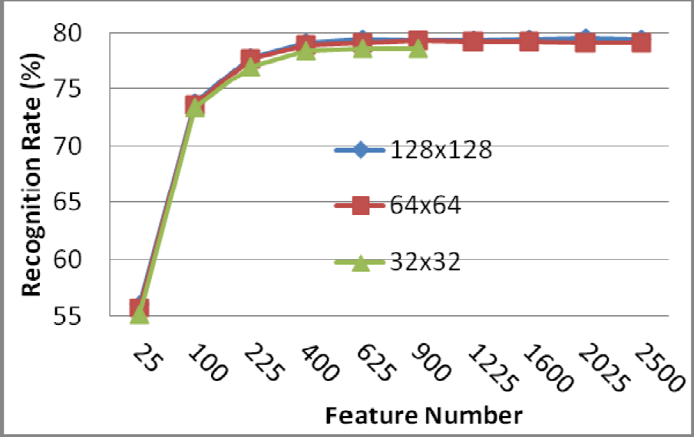
Effect of changing the feature number with the Global DCT method on recognition
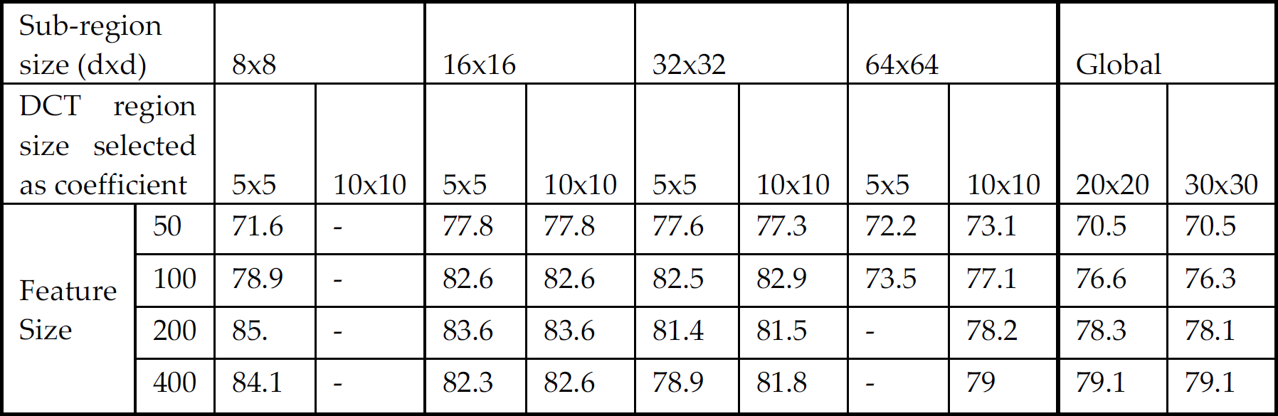
With the local DCT method, face images in 3 different dimensions were also used. In order to apply the local DCT method, these images were re-separated into sub-regions varying between 8×8 and 64×64 dimensions. Within each sub-region, the coefficients changing between the lowest frequency 2×2 and 6×6 dimensions were selected and used as features. As the results which are demonstrated in Table 2 are examined, it emerges that the recognition rate is not fixed for any given parameter but rather that it is dependent on all of the parameters to a certain extent. Moreover, the use of greater numbers of coefficients does not necessarily elevate the recognition rate.
Recognition rate for changing the coefficient size with the Global DCT method

3.3.2 Feature Selection
In sub-space-based methods, not all conversion factors possess a recognition-enhancing effect. The use of conversion factors collectively – regardless of the non-presence of a dimension problem – does not constitute a proper approach because certain base images are contingent upon factors like expression changes on the face. In case of use they lower the recognition rate. Via feature selection methods, the recognition rate can be increased by discarding the coefficients with low levels of discriminativeness. Another objective of feature selection is to lower the dimension. Irrespective of the fact that methods like Independent Component Analysis and DCT condense information on particular coefficients, the dimension of the obtained coefficients may be greater. With discriminative methods – such as Mahalonobis or LDA, which are especially used in classification – this may result in an inability to take the reverse of the covariance matrix, which is largely related to the smallness of the training set number. In practice, on the other hand, the number of training sets is generally far from adequate.
A substantial number of pattern recognition methods have not been designed in such a way as to discard irrelevant features. On account of large-scale data, this has been a requisite in order to select features in biometric applications.
The objective in feature selection is to obtain a d scale Xopt={xk | k=1,..,d} subset out of the D scale Y={yj | j=1,..,D} set with the aim of maximizing the J(Xopt) criterion. The optimum subset can be found by trying a 2d probability; however, this is not applicable enough for practical problems. This is why suboptimal methods are preferred.
Saey et al. [28] classified feature recognition into three sub-groups, namely filter, wrapper and embedded. Filter methods look into account the self-qualities of features. Its advantages are related to its applicability to large-scale databases and its speed. The disadvantage is that it fails to use the correlation between features. A good number of filter methods utilize class discrimination value as the performance criterion. Among these methods, the most frequently-used one is that of Fisher Discrimination Value (FDV).
In order to determine the class discrimination power of each coefficient via FDV, the ratio of the interclass variance of each coefficient to the interclass variance is utilized [29, 30, 31].
If class average for j. is represented with x̄j in-class variance:
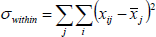
where x̄ is the means of all coefficients, and interclass variance:


Out of the input data l the term with the highest classification power is selected, and by combining all of these terms, a feature vector is created:

3.3.3 Feature Selection out of Global and Local 2D DCT coefficients
With 2D face recognition, the recognition process has been achieved by selecting low-frequency terms, mostly from 2D DCT coefficients. In the current study, on the other hand, 2D conversion factors were separated into different band regions to determine the class discrimination power of each band individually [25]. The coefficients that were selected with respect to each band with a different power of class discrimination were utilized as feature vectors. Unlike the rest of the studies, by computing the class discrimination power of every single DCT coefficient, the most discriminating n={50,100,200,400} feature was used for recognition. In Table 3, after computing the DCT coefficients of a 128×128 size image, the selected n coefficient from the low frequency {5×5, 10×10, 20×20, 30×30 block was employed as the feature. An ‘n’ quantity of increase in the number of the selected feature did not necessarily elevate the success for all of the sub-regions; it even reduced the recognition rate to a certain extent, which may be attributed to the fall in the generalizing capacity of high-frequency coefficients.
The change of the recognition rate with the global and local DCT methods with respect to the change in the number of features
3.3.4 Linear Discriminant Analysis and Classification
Prior to the classification process, and in order to increase the distance between the classes even further, all of the feature vectors were used as a unity and LDA was conducted. The WLDA matrix computed via the LDA method was multiplied by the y feature vector and the new feature vector Y'=WLDA×Y was obtained. The objective was to use the conversion matrix (det(Sb)/det(Sw)), optimizing the ratio between the inter-class matrix (Sw) and the in-class matrix (Sb) [32]. In-the class matrix:
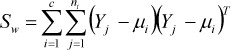
and the inter-class matrix:
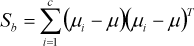
where c stands for the number of the class, ni i stands for the number of faces in the class, Yj represents j. feature vector of class, μi represents i. the feature vector means of class, μ represents the means of all classes. WLDA is the eigenvector of the SbSw−1 matrix.
3.3.5 Experimental Results with Linear Discriminant Analysis
In the previous section, the recognition rate was increased to 83% by selecting the features with respect to their discrimination. Once the LDA was conducted over the selected features, the recognition rate increased to above 97%.
3.3.6 Detecting the optimum feature size
As the findings shown in Table 4 are analysed, it emerges that in terms of both local DCT and global DCT, the rise in the number of features does not increase the recognition rate; indeed, it even reduces the recognition rate. This is because high frequency coefficients are more dependent on the noise in the image which affects the success adversely. It is not possible to use high frequency as well as low frequency coefficients collectively as features. Some of these coefficients are reliant on factors such as illumination or facial expression; hence, the most discriminative coefficients need to be selected and used as features.
The change of the recognition rate in relation to global and local DCT methods after LDA was applied with respect to a change in the number of features

The features of the image of which the DCT coefficients are computed after dividing into 32×32 size sub-regions were selected and utilized for recognition. In Figure 7, we see that the recognition rate changes with respect to the number of selected features. The highest recognition rate was achieved for 170 coefficients. The increase in the recognition rate was not parallel to the increase in the number of features, even though the opposite holds true. This outcome is described as the “curse of dimensionality” in image processing [33]. The utilization of higher numbers of features reduces the success of generalization.

Change in the recognition rate with respect to the number of selected features
In Figure 8(b), the positioning of the coefficients selected from the sub-regions is symmetrical with respect to the vertical axis, which is attributed to the fact that the face is symmetrical alongside the vertical axis passing through the nose and the right and left sides of face bear almost the same discriminative values.
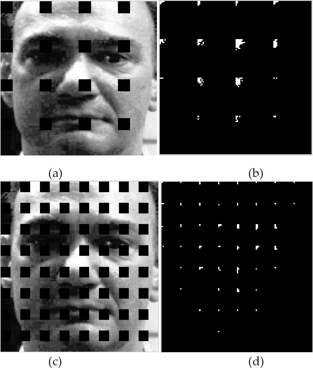
Sub-regions (a,c) and coefficients selected from each sub-region (b,d)
The face was divided into sub-regions and the coefficients selected from each sub-region are demonstrated in Figure 8. By exploring the intensity of the coefficients selected from every single sub-region, it is feasible to determine the degree of discriminativeness of the relevant region. Attention is drawn to the fact that the most discriminant coefficients are centred on the eye and nose areas. The discriminativeness of the mouth, cheek and forehead regions, however, are lower than with the eyes and nose. The eyes and nose – on account of being the areas that are most sensitive to changes of expression – possess higher numbers of discriminating features. Previous methods established recognition by using a fixed quantity (such as 3×3) of coefficients as features. The use of a fixed quantity of coefficients should give way to the selecting of noisy coefficients from non-discriminative areas, like the cheeks and the forehead.
4. Experimental Studies for the DSP
The algorithm running over the DSP is made up of two parts, namely face detection and face recognition. In the literature, two methods are followed in order to develop software in embedded systems. With the first method, the algorithm is developed on a general-purpose PC and optimized for preset hardware. With the second method, the algorithm is directly and exclusively developed for the preset hardware. For the present research, we selected the first method and used the environment presented in Figure 9. Although the memory and processor power create no problem on a general-purpose PC, in embedded systems these resources are limited. However, it was preferred to test the algorithm after development without these restrictions and then to customize it upon successfully achieving our targets. To this end, we developed the algorithm in a PC environment and then optimized for the DSP.

(a) Block schemes for the tools used in the experiment (b) Face detection experimental setting
4.1 Face Detection and Recognition on the DSP
The Viola-Jones face detector was tested for face detection. This method was run on computer and a DSP but the operational period was restricted to minutes. In order to speed up the algorithm, tests were conducted on both a PC and a DSP. In the aftermath of all these tests, the parts of the algorithm that demanded the greatest operation were examined. During these tests, the most frequently called upon functions were identified by taking logs. Since the PC was not operating in real-time and was inaccessible throughout the process cycle, in order to determine the cycle lengths we used the free running timer of the DSP. At the end of the analyses, the steps that required the greatest number of processes were detected: 1) the floating point processes, 2) the floating point square root, 3) the integral image, and 4) because of the random characteristics of Haar features, the increase in the time taken to access the memory
The first problem stems from the fact that the DM6437 processor bears a fixed point ALU. It is capable of floating point processes, however, since it can manage this process with the help of a program – the fixed point multiplication that can be completed in one cycle alone rises to 40–50 cycle lengths. The same problem holds true for other arithmetical operations and comparison processes. To solve this problem, the highest and smallest threshold values of floating point processes and the required accuracy were analysed. The floating point variables in the program were multiplied with the matching constants, converted into whole numbers and then used. In our tests, this method mostly functioned well but failed to function properly with some images. As we investigated the error in the program, we detected that the problem was related to overflow. To overcome this problem, the variables were defined as a 64-bit “long integer”. Therefore, it became possible to obtain variables with great dynamic intervals and their resolution was enhanced. Since the DM6437 was fixed on a 64-bit pipeline, the length of its cycle remained almost unchanged.
The second problem involves the required processing power to take the square root of the floating point. The research conducted has demonstrated that the same problem was also encountered in graphic processing and that to overcome this problem a very fast square root taking method was developed [34]. This method became particularly popular in the aftermath of 2005 and it has currently found a place as the 2-cycle Assembler instruction in the architecture of the TI C66x. Nonetheless, since the DM6437 processor runs a fixed point, it fails to operate the Newton-Rapson process used in this method quickly enough. On that account, a different method was employed. Reminiscent of the SAR (Successive Approximation Register) method, it starts from the highest bit by taking the square of the variable and it is compared with the number of whichever square root will be taken; if the number is small, it increases the smaller value bit which comes next and detects the square root of the number. At this point, and in order to boost the processes, it is necessary to determine the bit which will be compared. The analyses showed that the numbers changed between the 50–2000 interval; hence, by adding the margin of safety to the comparison and starting from the 12th bit (2000 < 4096=212), the 20(32–12) bit of the redundant process was discarded.
In the Viola-Jones method, the integral image is a salient approach which enables the rapid computation of Haar features. Once the integral image is computed, the computation of Haar features in different scales can be made possible by changing the Haar coordinates. Unlike other object detection methods, it is not necessary to compute the conversion repeatedly for every new scale. This is the basic reason accounting for the most distinguishing factor of the Viola-Jones method, namely that it runs quite fast on different scales. In the present study, the Haar feature coordinates were also computed once and then registered, since the dimensions of the frames inside the video were all the same. Inside each frame, the search was conducted for the same scales. Since Haar feature coordinates are independent of the image, one-time computation was sufficient. At the end of the first frame, those variables which were solely dependent on image were recomputed. Among these variables, the step that demands the highest power of processing is the computing of the integral image. A fast computation could be achieved by taking into consideration the characteristics of the integral image and the advantages of a 64x+ architecture.
One of the most significant restrictions determining the speed of any algorithm is memory size. Although the DM6437 can work with 4GB of external memory, in the system which we used only 128MB of external memory was available. There are 128kB L2/SRAM and 112kB L1/SRAM. The L1/SRAM access time of the processor is 1 cycle, the time to access L2/SRAM is 4 cycles and the time to access the external memory is over 50 cycles.
Accordingly, the memory requirement for the integral image of video frames is 576×704×4=1.6MB. In this case, the L2 memory falls short. It would constitute only a slight possibility were we to seek the needed data in the L2 memory. This is because the corner coordinates of the Haar features do not change synchronously. For almost every single block, a page-fault emerges; hence, access to external memory is required. We experimentally observed the consequences: the increase in the cycle lengths. As a remedy, it would be possible to utilize a DSP with adequate L2 memory; however, and as regards the DM6437, this problem will continue.
The image splitting approach which is utilized in embedded video processing was also analysed. As a solution, it is required of every single scale that it divide into matching sub-regions in changing sizes. In this case, the algorithm shall become more complex and the time needed for data transfer and the compilation of findings will increase. Accordingly, this approach was discarded. After the face detection stage, the detected faces are transferred to the face recognition algorithm. Prior to recognition, the faces are subject to histogram equalization in order to diminish the effect of illumination. Face images are resized to 128×128 and DCT is applied to extract the features. Resizing and histogram equalization processes require less processing power than the DCT.
The next action is the feature selection. Feature selection has two stages: training and usage. Training is an offline process and does not need to be in the DSP – it can be realized on a PC. Once the discriminating features have been determined, that information is saved into a file and used in the feature selection process. To this end, the DSP reads this file at start-up and uses the information provided during the feature selection stage. Therefore, the feature selection process requires much less processing power from the DSP than the other processes.
The next step is Lineer Discriminant Analysis. Like feature selection, a LDA transformation matrix is calculated offline on a PC and saved onto a file. The DSP loads this file before start-up and uses it in the next process. LDA is a simple matrix multiplication and performs very quickly on the DSP.
4.2 Operational Performance
The face detection and recognition method developed in a PC environment was then optimized for the DSP and then run on it. The tests were conducted over an image extracted from a 576×704 size input video on the DSP. To conduct face detection and recognition, for a 600Mhz DSP processor the operational time is around 1 second and the vast majority of this time is dedicated to the face detection program. Due to the great size of the image, face detection takes longer. In commercial systems, large-scale images – in order to increase the speed – are down sampled for searching. The most popular size is a standard video size of 240×320 (QVGA). Although the face detection program detects multiple faces, only one of these faces is used for recognition.
The face recognition algorithm consumes a 65M cycle in terms of processing power, which takes 108ms on a 600MHz DM6437 DSP. A 58M cycle is used for the calculation of the DCT coefficients. The remaining cycle is used for resizing, histogram equalization, feature selection and LDA. The DCT calculation of 16 32×32 sized windows requires a 524,288 (16×32log32×32log32) floating point processing cycle. Since the DM6437 is a fixed point processor, it actually consumes many more cycles than the given number.
5. Conclusions
In the present study, a face detection and recognition system operating in a DSP was developed. To detect faces, the Viola-Jones method was tested. To obtain face recognition, the qualities of the facial regions in the image were retrieved. Different approaches were tested for feature extraction. In previous studies, the features were extracted from facial images via global DCT or local DCT and the lowest frequency coefficients bearing the most information were selected for recognition. In the current study, however, those coefficients with the most discriminative characteristics (rather than those with the most information) were selected for recognition. In the conducted research, it was observed that the most discriminative coefficients were basically centred around the nose and eye regions, which were the least sensitive areas against changes of expression. Quite low numbers of coefficients from the chin, mouth and forehead areas were selected as features.
Tests of the method developed for a DSP were executed on the PC. Test-purpose face recognition experiments conducted on the FRGC database yielded a 97.4% success rate. By splitting the face image into sub-regions, changing quantities of discriminative coefficients were selected from each sub-region.
Certain parts of the method's development and the relevant tests were executed in a PC environment. DSPs – as compared to PCs – bear particular advantages and disadvantages. The most striking disadvantages are their fixed point processor and their restricted memory. In the present study, the floating point process requiring the Viola-Jones method was analysed, the most frequently repeated steps were optimized for the DSP, and a number of processes were optimized for a fixed point processor.
By making use of a fixed image size for the video, Haar feature information computed for a particular image size was used for those images retrieved from the whole video. The measurements that we conducted over the DSP proved that, thanks to optimization, the system worked 3 times faster. It takes around 1 second to retrieve results on the DSP from the image transmitted by the camera. A substantial part of this time is used for face detection. Although the size of the image was larger compared to the rest of the studies, it needs to be even further reduced. To this end, it is necessary to further parallelize the application steps of Haar features, especially for DSPs.