
Abstract
In this paper, precise control of the end-point position of a planar single-link elastic manipulator robot is discussed. The Timoshenko beam theory (TBT) has been used to characterize the structural link elasticity including important damping mechanisms. A suitable nonlinear model is derived based on the Lagrangian assumed modes method.
Elastic link manipulators are classified as systems possessing highly complex dynamics. In addition, the environment in which they operate may have a lot of disturbances. These give rise to special problems that may be solved using intelligent control techniques.
The application of two advanced control strategies based on fuzzy set theory is investigated. The first closed-loop control scheme to be applied is the standard Proportional-Derivative (PD) type fuzzy logic controller (FLC), also known as PD-type Mamdani's FLC (MPDFLC). Then, a genetic algorithm (GA) is used to optimize the MPDFLC parameters with innovative tuning procedures. Both the MPDFLC and the GA optimized FLC (GAOFLC) are implemented and tested to achieve a precise control of the manipulator end-point.
The performances of the adopted closed-loop intelligent control strategies are examined via simulation experiments.
1. Introduction
Establishing increasingly complete and accurate dynamic models and synthesizing efficient control schemes for the special category of elastic link manipulators are two extremely challenging and still-open problems in robotics research.
Compared with conventional rigid robots, elastic link manipulators have special potential advantages of larger work volume, higher operation speed, greater payload-to-manipulator weight ratio, lower energy consumption, better manoeuvrability and better transportability. However, they also encounter deformation and vibration typically associated with the structural elasticity, and as a consequence their dynamics modelling is made extremely complicated.
The complexity of modelling and control of this class of lightweight manipulators is widely reported in the literature. Detailed discussions can be found in [1]–[7].
An accurate, dimensionally finite and mathematically complete model based on a detailed understanding of all variables in the process is strictly required by the different conventional control schemes applied to such robots. These model-based controllers, originally designed for the demands of high performance, may not be easy to implement in elastic arm control practice, due to uncertainties in design models and large variations of robot hand loads, the ignored high frequency dynamics (related to control and observation spillovers), and the high order of the designed controller. So, it is highly desirable to find simple and robust controllers which eliminate the need for an accurate mathematical description of the plant to be controlled.
The focus of this article is mainly on the application of alternative closed-loop intelligent control strategies, including fuzzy logic, to try to obtain precise and robust motion of the end-point of an elastic single link robot manipulator arm modelled by the use of the TBT. For this purpose, two advanced control schemes are proposed: a PD-type Mamdani's FLC and a GAOFLC.
The remainder of this paper is organized as follows. In Section 2, we briefly review the basics of fuzzy logic control and the genetic algorithm optimization method. A brief review of the TBT is also given. In Section 3, a comprehensive dynamic model of the studied robot is obtained after its physical configuration is presented. In Section 4, we present the derivation and the application of the first adopted feedback control scheme: a fuzzy-like PD controller abbreviated here by MPDFLC. Simulation results are also presented. In Section 5, a GA is used to optimize the MPDFLC parameters with some innovations in the tuning procedures. The performances of the resulting GAOFLC are examined via simulation experiments. Section 6 concludes the paper.
2. Preliminaries
2.1 Brief review of fuzzy logic control basics
In standard set theory, an object is either a member of a set or it is not a member at all. Given a universe of objects U and a particular object × e U, the degree or grade of membership μA (x) with respect to a set A⊆B is:

The function μA(x):U→{0,1} is called characteristic function in standard set theory. Often, a generalization of this idea is used, for instance to handle data with error bounds. A degree of membership of one is assigned to all the numbers within an error percentage, and all the numbers outside that interval are assigned a degree of membership of zero (Fig. 1(a)). In precise cases, the membership degree is set to one at the exact number and zero everywhere else (Fig. 1(b)).

Membership functions for crisp and fuzzy data
In 1965, Zadeh [8] proposed a further generalization in which some objects have a greater degree of membership of a set than others.
The degree of membership takes on various values between zero and one, where a zero value indicates complete exclusion and a value of one indicates complete membership. This generalization allows more precise expression. For instance, to express that a temperature is around 25, we may use a triangular membership function (MF) with its peak at 25 to express the idea that the closer a number is to 25 the better it qualifies (Fig. 1(c)).
Formally, let U be a collection of objects denoted generally by {u}. U is the universe of discourse (UD) and may be continuous or discrete. A fuzzy set A in a universe U is defined by an MF μA which takes values in the interval [0,1]μA:U→[0,1] . We can also define a fuzzy set as a collection of ordered pairs of a generic element u ∈ U and its grade of MF μA (u), i.e.,
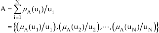
where N is the number of elements of U and the symbol Σ denotes collection of discrete elements. The corresponding notation for a continuous UD U is

The support of a fuzzy set A is the crisp set of all points u in U such that μA > 0. A fuzzy set whose support is a single point in U with μA = 1 is called a fuzzy singleton.
In several fuzzy sets applications, we often encounter situations where two or more fuzzy sets are involved. Thus, formal treatments of fuzzy operations are needed. Below are some important treatments.
Let A and B be two fuzzy sets in U with membership functions (MFs) μA and μB, respectively.
The union (A∪B) and the intersection (A∩B) are defined by

or in terms of MFs by

The MF of the complement of a fuzzy set A is defined by

It is quite common to use qualitative phrases instead of quantitative values for words that denote measures and counts, such as fairly high, quite a few, not many. This idea is captured in the concept of a linguistic variable [9].
A linguistic variable takes on one of a set of labels, i.e., words or phrases, as its value. For example, the linguistic variable Temperature could take one of the members of the set (low, medium, high) for its value. The labels are given meaning by associating with each one a fuzzy subset (FS) of some UD (see Fig. 2).
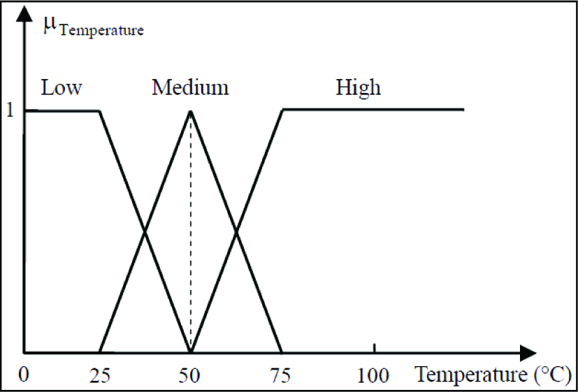
Linguistic variable Temperature
The structure of a process controlled via an FLC [10] is shown in Fig. 3. The basic constitutive components are:

Basic structure of fuzzy logic control
The fuzzification interface gets the values of input variables, performs scale mapping to transfer the range of values of input variables into corresponding UD, and performs the function of fuzzification to convert input crisp data into fuzzy values.
The knowledge base comprises a rule base characterizing the control policy and goals and the data base providing the necessary definitions about discretization and normalization of universes, fuzzy partition of input and output spaces, and MF definitions.
The inference procedure processes fuzzy input data and rules to infer fuzzy control actions employing fuzzy implication and the rules of inference in fuzzy logic.
The defuzzification interface performs scale mapping to convert the range of values of universes into corresponding output variables, and transformation of a fuzzy control action inferred into a nonfuzzy (crisp) control action.
Usually the fuzzy control rules are expressed in the form of a fuzzy conditional statementRi:
The fuzzy rule Ri can be regarded as a fuzzy relation from universe (U And … And V) to universe W. If there are n rules, the rule set may be represented by a union of these rules: R = R1 ∪ R2 ∪ … ∪ Rn. The resultant w can be induced by the compositional rule of inference [11]

where o denotes the compositional rule of inference. For example, using the sup-min compositional rule, we have:

The most frequently used fuzzy inference methods in fuzzy control are Mamdani's fuzzy implication and Larsen's product fuzzy implication [12]. If the fuzzy variables u, v, and w are fuzzy singletons, the inferred results of both implication methods will be the same:

where u0, v0, and w0 are fuzzy singletons and Ci is the singleton value of w using the i th rule.
After a fuzzy control action is inferred, a nonfuzzy control action that best represents the decision is needed. Although there is no systematic procedure to choose a defuzzification strategy, the most common include the MAXimum criterion method (MAX), which produces the point where the MF of the control action reaches a maximum value, the Mean-Of-Maximum method (MOM) which represents the mean value of maximums when they are not unique, and the Centre-Of-Gravity (COG) which generates the centre of gravity of the MF area of the control action (see Fig. 4).

Defuzzification strategy
2.2 Genetic algorithms
Based on Darwin's evolutionary theory [13], genetic algorithms were proposed by the computer scientist John Holland [14] in his quest for a general way of creating software solutions by evolutionary adaptive processes.
A genetic algorithm (GA) is a global search metaheuristic used to solve optimization problems.
The process of a GA (Fig. 5) consists of evolving an initial set of points, i.e., an initial population of randomly generated individuals (chromosomes), encoding solutions to the considered optimization problem to be solved towards final exact or approximate solutions. This process is executed by iterating a population with a constant size N. The evolution of the successive populations from a kth generation to a (k+1)th generation is based on the operations of selection, crossover and mutation, which are inspired by evolutionary biology [15]:

General principle of a genetic algorithm
Selection: A proportion of the population is selected from each successive generation to breed a new generation. The two most-used and well-known selection methods are roulette wheel selection and stochastic remainder without replacement selection.
Crossover: After the selection operation, the crossover operator reproduces new individuals from parents chosen with a probability Pc from among the surviving individuals. Three principle techniques are usually adopted: the slicing crossover, the k-point slicing crossover, and the uniform crossover.
Mutation: This operation refers to a random change (mutation) with a probability Pm in some selected chromosomes to escape local optima and ensure accessibility of the entire solution space.
These operations or genetic operators act on all the kth generation individuals. For each generation, the GA selects the best individuals according to an adaptation or a fitness which is the cost or optimization function.
2.3 Brief review of the Timoshenko beam theory (TBT)
A rigorous mathematical model widely used for describing the transverse vibration of beams is based on the TBT [16], developed by Timoshenko in the 1920s. This partial differential equation (PDE) based model is more accurate in predicting the beam's response than a model based on the classic Euler-Bernoulli (EB) beam theory [17]. Indeed, it has been shown in the literature that the predictions of the Timoshenko beam (TB) model are in excellent agreement with the results obtained from the exact elasticity equations and experimental results [18].
A historical review of the different beam theories and their specifications can be found in [19].
The TBT accounts for the effect of both rotary inertia and shear deformation, which are neglected when applied to EB beam theory. The transverse vibration of the beam depends on its geometrical and material properties as well as the external applied torque. The geometrical properties refer mainly to the length l, size and shape of the cross-section such as area A, moment of inertia I with respect to the central axis of bending, and Timoshenko's shear coefficient k, which is a modifying factor (k<1) to account for the distribution of shearing stress such that effective shear area is equal to kA. The material properties refer to the density in mass per unit volume ρ, Young's modulus or modulus of elasticity E and shear modulus or modulus of rigidity G [19].
3. Dynamic Modelling of the Elastic Robot Manipulator
3.1 The elastic link robot system
The studied robot manipulator physical system is shown in Fig. 6.

Physical configuration of the elastic robotic arm
The system consists of a clamp-free planar moving elastic arm with tip payload, which can bend freely in the horizontal plane.
The axis of rotation of the rigid hub (Z0) is perpendicular to the robot evolution plane. The X0–Y0 coordinate frame is the inertial frame of reference. That indicated by X – Y is a frame of reference that rotates with the overall structure. The X -axis is tangent to the link at the base.
Considering, as usual, the elastic link as a beam, its cross-section height is assumed to be larger than the base. This constrains deflections w(x,t) to occur only in the horizontal plane. Thus, those due to gravity are assumed negligible.
The robot manipulator is essentially composed of a rigid hub, an elastic link and a payload. The rotating inertia of the actuating servomotor and the clamping rigid hub are modelled as a single hub inertia Jh. The payload is modelled as an end mass Mp with a rotational inertia Jp.
The rotating X -axis angular position (angular position of the hub) being θ(t), that of the point of the deflected link, α(t), is given, for small deflections, by:

3.2 Governing equations of motion
The kinematics of deformation of an element of the deflected link with width dx at position x are shown in Fig. 7.

Kinematics of deformation of a bending element
This element undergoes a shearing force S(x,t) and a bending moment M(x,t).
The deflection is due to both bending and shear forces, so that the shear angle σ(x,t) (or loss of slope) is equal to the slope of centre-line (neutral axis)

The shear force S and the total internal moment (bending and damping) M are given in [19]:
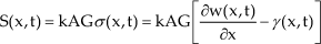
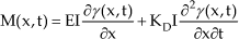
where KD is the Kelvin-Voigt damping coefficient.
The equations of motion of the studied elastic robot can be derived by considering both the equilibrium of the moments and the forces given by
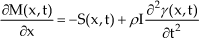
where AD is the air damping coefficient.
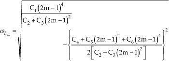
After some manipulations, detailed in [19], we obtain the fifth-order TB homogeneous linear PDE with internal and external damping effects expressing the deflection w(x,t) (Eq. 16).
Initial and clamped-mass boundary conditions (Eq. 17 -Eq. 21) are assigned to this PDE representing the motion equation of the damped TB [19].

– Initial conditions:

– BCs at the clamped end (root of the link):
* Zero average translational displacement:

* Zero average of bending moments:

– BCs at the mass-loaded free end:
* Zero average of bending moments:

* Balance of shearing forces:

Based on the assumed modes method [17], w(x,t) can take the following expanded, separated form, which consists of an infinite sum of products between transverse deflection eigenfunctions or mode shapes Wm(x) that must satisfy the considered boundary conditions, and time-dependant modal generalized coordinates δ n (t):

Assuming a first set of mode shape candidates as

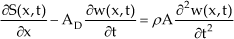
the expression of the robot link transverse displacement w(x,t) is established by substituting (22) with (23) into (16) with some approximations (see [20]) as

where the most important parameter is the damped frequency
The final clamped-mass mode shape functions have been derived based on the important results established in [21, 22]. Indeed, it has been demonstrated by comparative studies that, at the first low frequencies, the mode shapes and the vibration frequencies of the EB beam and the TB are very close.
Inspired by these works, we have proposed [23] to adopt the mode shapes of a damped EB beam [24] with
The clamped-mass mode shape functions are given by:

with

Ωm has been calculated based on a suitable normalization satisfying
3.3 Dynamic model
In order to obtain a set of ordinary differential equations (ODEs) of motion to adequately describe the dynamics of the elastic link manipulator, the Lagrange approach combined with the assumed modes method [26] is used.
According to the Lagrange method, a dynamic system completely located by m generalized coordinates qi must satisfy m differential equations of the form

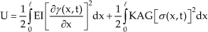
where L is the so-called Lagrangian, given by

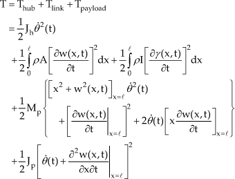
T represents the kinetic energy of the modelled system given by
U represents the system potential energy and D the dissipative effects. These are, respectively, given by

Fi is the generalized external force acting on the corresponding coordinate qi.
Substituting the energies expressions into (26) accordingly, using the transverse deflection separated form (24) and truncating the number of ODEs (modes) at 2 [19, 27], we can, after tedious manipulations, derive the desired dynamic equations of motion in the mass (B), damping (H) and stiffness (K) 3 × 3 matrix form:
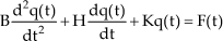
with

where

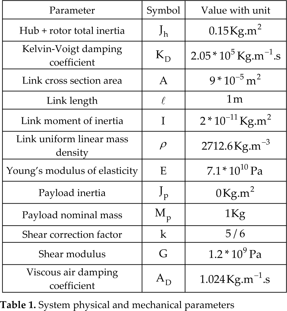
For the purpose of digital simulations, the following physical and mechanical parameters [28], given in Table 1, have been adopted. The simulation study will be conducted using the Matlab-Simulink software.
System physical and mechanical parameters
4. Controlling the Elastic-Link Robot Manipulator by a PD Type Mamdani's FLC
The FLC based end-point control of the elastic-link robot manipulator adopted in our work is illustrated in Fig. 8. It is well known by Mamdani's FLC [29]. This scheme, by its structure, is also called “PD type FLC” where PD stands for Proportional-Derivative.

MPDFLC-based manipulator feedback control scheme
The FLC input variables are the loop error e and its rate of change Ae, defined as:

where αRef is the desired tip angular position and mT is the mth sampling instant,

The change in the control setting is denoted by Au(mTs). Ge and GΔe are the input scaling factors and GΔu is the output scaling factor. Thus, the PD type fuzzy logic command is given by

After a long series of trial-and-error tests, the PD-type Mamdani's FLC characteristics have been fixed as:
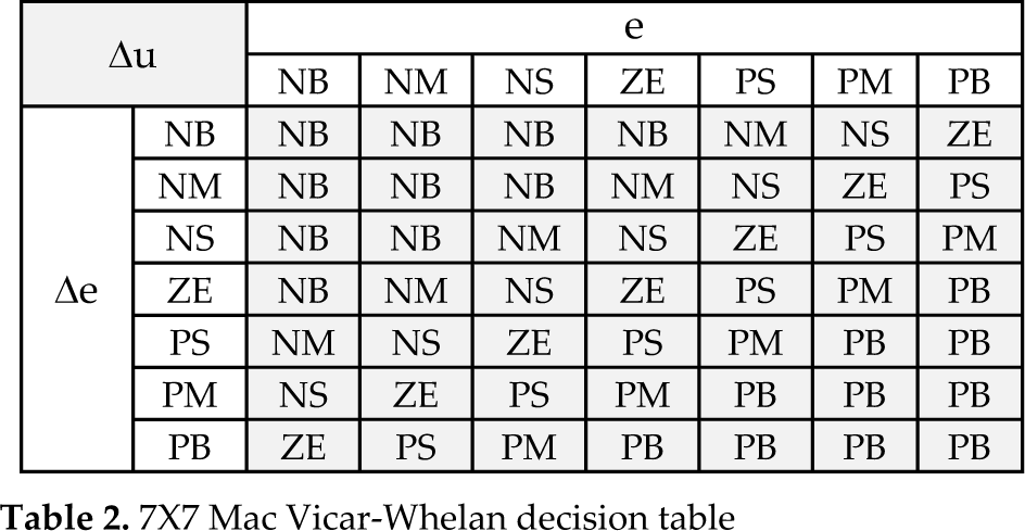
Seven FSs have been chosen to describe the error, its rate of change and control variation amplitudes. As seen above, their linguistic formulation and symbols are defined in the usual fuzzy logic terminology by: Positive Big (PB), Positive Medium (PM), Positive Small (PS), Zero (ZE), Negative Small (NS), Negative Medium (NM), Negative Big (NB). The “meaning” of each linguistic value should be clear from its mnemonic.
The set of decision rules forming the “rule base” which characterizes our strategy to control the studied dynamic process is organized in a matrix form (see Table 2) based on Mac Vicar-Whelan's diagonal decision table [30].
The same triangular shapes have been assigned to the MFs of the FLC variables with a uniform distribution. A 50% overlap has been provided for the neighbouring FSs. Therefore, at any given point of the UD, no more than two FSs will have a nonzero degree of membership.
For greater flexibility in FLC design and tuning, the universes of discourse for each process variable are often “normalized” to the interval [−1,+1] by means of constant scaling factors. The best scaling factor values have been determined by a tedious trial-and-error process as Ge=0.52, GΔe=0.49 and GΔu=11.1.
The adopted inference method is based on the Mamdani's Implication mechanism, and is also called the SUPremum-MINimum composition principle [12].
To obtain a crisp value of the inferred fuzzy control action we have selected the COG defuzzification technique, which has been successfully used in several applications [31].
7×7 Mac Vicar-Whelan decision table
The response of the elastic arm corresponding to 90° step input and the generated control input are presented, respectively, in Fig. 9 and Fig. 10.

MPDFLC-based step response with reference angle 90°
MPDFLC-based generated control input
The MPDFLC used to enforce the desired angular position successfully converges the system output (end-effector) to the desired position with an acceptable delay (less than three seconds) and maintains it at the reference without overshoot, undershoot or residual vibration.
To try to improve the obtained performance, the proposed GAOFLC application is presented in the next subsection.

or in discrete form

where k0 and kf are the initial and final discrete times of the evaluating period and Ts is the sampling period.
5.1 Derivation of the GAOFLC
To try to improve the performance obtained with the MPDFLC design based on a trial-and-error process, we use the GA as an evolutionary optimization method [33, 34] to automatically adjust the following parameters:
Number of MFs for each FLC variable
MFs shapes for each FLC variable
MFs distribution for each FLC variable
Decision table rules
Scaling factors.
5. Controlling the Elastic-Link Robot Manipulator by the GAOFLC
The GAOFLC-based feedback control system architecture is shown in Fig. 11.

GAOFLC-based feedback control system architecture The mathematical expression of Of is written as:
The FLC being codified as a chromosome, the GA optimization process starts with a first FLC (initial solution) and begins the iterative evaluation of the generated new solutions by an objective function Of.
Of is chosen to maximize the inverse of the best-known and most-adopted performance index: Integral of Time-weighted Absolute Error (ITAE) [32], abbreviated here by DITAE.
5.1.1 Conception hypotheses and constraints
Certain assumptions and constraints about the decision table and the FLC variables MFs to be optimized are given here:
The number of FSs (NFS) for each variable can take only one of the following possible values: 3, 5, 7 or 9.
The FSs will be symbolized (labelled) by the standard linguistic designation and indexed in ascending order. If, for example, the number of FSs of a linguistic variable is equal to 5, the corresponding FSs will be NB, NM, ZE, PM and PB, and indexed from 1 to 5. The FSs NB and NM are considered as the opposites to PB and PM respectively (symmetrically with respect to ZE).
Note that the label ZE stands for linguistic (fuzzy) value zero, first letters N and P mean negative and positive and second letters B, M and S denote big, medium and small values, respectively.
All the FLC variables universes of discourses are normalized to lie between-1 and +1.
The first and the last MFs have their apexes at −1 and +1, respectively.
5.1.2 Decision rules table deriving method
The method on which we have based the decision rules table is inspired by [35, 36], where a kind of grid is proposed.
This paper proposes a new method of FS assignment to each of the grid nodes in the special case of equality of distances between the points representing the candidate decision rules (see the decision rules table deriving method principle given below). Note that this new procedure is adopted instead of the random assignment proposed in [36].
Principle of the method
First, the grid is constructed using two spacing parameters PSGe and PSGΔe relative to the FLC two inputs e and Δe.
The first (resp. the second) spacing parameter PSGe (resp. PSGΔe) fixes the grid node X-axis coordinates (resp. Y-axis coordinates) in the interval [−1, +1] (UD) with a simple computing formula given in the next paragraph. Each abscissa (resp. ordinate) represents an FS of the variable e (resp. Δe). The number of the grid constitutive nodes is then equal to the product result between the two FLC input FS numbers.
Once the nodes are fixed, we introduce the output points on a straight line corresponding to the FLC output variable Au. Now, the points (output) represent the FSs and not their coordinates. The number of points is equal to the output variable FS number.
A third spacing parameter PSGΔu fixes the output point X-axis (Y-axis) coordinates similarly, whereas the Y-axis (X-axis) coordinates are calculated by an angular parameter, noted “Angle”. This determines the slope of the straight line supporting the output points with respect to the horizontal. This angular parameter varies in the interval [0,π/2] anticlockwise.
Each of the grid nodes represents a case of the decision table and each output point represents an FS of the control variable Au.
Once all the point coordinates (grid nodes and output points) are computed, we can proceed to the assignment by determining the minimal distance among all the distances separating each node of the grid from all the output points situated on the straight line. Then, we assign to each node of the grid the closest output point. Consequently, the decision table case corresponding to this node will contain the FS representing the selected output point. Nevertheless, an assignment conflict could arise in the case of equality between two minimal distances separating a node and two output points. We propose to select the output point which has the lower FS index in the case of the upper part with respect to the table diagonal, or the output point which has the greater FS index in the case of the lower part. It should be noted that no more than two output points can be at the same distance from a given node of the grid, since all the output points are on the same straight line.
Spacing parameter
The grid spacing parameter PSG specifies how the positions Ci of the intermediate points (between the centre and the extreme of each graduated axis) are spaced with respect to the central point.
This parameter offers flexibility to vary spacing. The more it is greater than 1, the more the point positions are close to the centre and vice versa. At the value 1, the positions are uniformly distributed in the UD interval [−1, 1].
The number of positions C being obviously the same as the number of FSs, we propose a formulation of the spacing law according to the spacing parameter PSG.
As a first stage, the positions Ci, being equidistant, are denoted by CEqi and computed by:

The Ci values are then determined in terms of the spacing parameter PSG as follows:
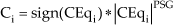
with
Two illustrative examples of C computation are given in Table 3 (seven FSs) and in Table 4 (five FSs) for different values of the spacing parameter.
Ci for PSG for seven FSs

Ci for PSG for five FSs

To understand the decision table deriving procedure, two detailed examples are given below.
The constructing parameters are given in Table 5. The grids and their corresponding decision tables are shown in Fig. 12 and Fig. 13, respectively.

Example 1: (a) Grid constitution for decision table construction. (b) Derived decision table

Example 2: (a) Grid constitution for decision table construction. (b) Derived decision table
Two illustrative examples

Note that the nodes are represented by red stars and the output points by blue circles. The purple arrows are examples of minimal distances between the output points and the grid nodes describing the FSs' assignment to the decision table.
It is interesting to note that the decision table obtained for PSGe =PSGΔe =PSGΔu =1 and Angle =45° is none other than the Mac Vicar-Whelan diagonal table [30].
5.1.3 Membership functions deriving method
Determination of the FLC MFs using the GA takes place in three phases:
Creation of primary MFs of the FLC input/output variables
Parameterization
Adjustment of the MFs.
MFs shape and width optimization
Three types of MF shapes are considered:
Triangular
Trapezoidal, which include (generalize) the triangular type
“Two-sided” Gaussian with flattened summit.
The triangular shape is defined by three parameters, [P1 P2 P3], which represent, respectively, the left abscissa of the triangle base, the peak abscissa, and the right abscissa of the triangle base.
Each triangle base begins at the preceding triangle peak abscissa and ends at that of the following one.
The trapezoidal shape is defined by four parameters, [P1 P2 P3 P4], representing, respectively, the base left abscissa, the summit left abscissa, the summit right abscissa, and the base right abscissa. It is then framed by four points with the coordinates (P1,0), (P2,1), (P3,1) and (P4,0) (see Fig. 14). Note that if P2 = P3, we obtain a triangular shape.

Trapezoidal MF
We also define the two-sided Gaussian shape by four parameters, [Sig1 G1 G2 Sig2] (see Fig. 15). The left and right sides of the Gaussian are respectively defined

Two-sided Gaussian MF
For that purpose, we adopted a very small positive real number ε (ε = 0.01 was quite suitable) such that:
The Gaussian left curve includes the points (P1, ε) and(P2,1)
The Gaussian right curve includes the points (P3,1) and(P4, ε).
This formulation leads to the establishing of the following two systems of equations:
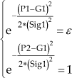

The resolution of systems (39) and (40) gives:

Note that ε has been used, since the two sides of the Gaussian never pass a null abscissa.
Width spacing parameter
The summit abscissae of the different shapes are calculated by the same principle of parameter spacing used in the determination of the grid nodes and point coordinates for the decision table derivation. The FLC input/output variable MF spacing parameters are, respectively, denoted by PSFe, PSFΔe and PSFΔu.
Shape optimizing parameter
The MF spacing method is inspired by the works of Park et al. [35], Foran [36] and Cheong and Lai [37]. The contribution of this paper is to propose a new technique for the MF shape optimization.
This technique is based on a design parameter called shape parameter (SP). This optimizing parameter gives possibilities of diversification (hybridization) of MF shapes on the UD of each of the FLC input/output variables.
SP is considered as a real number belonging to the interval [0, 2]. Its integer part, denoted by ISP, will determine the shape of the MF, and its fractional part, denoted by FSP, will determine the spacing with respect to the centre of the MF.
The MF shape is specified by ISP and FSP as follows:
The number of MFs (NFS) for each of the FLC input/output variables is optimized by the GA, and is not constant. Consequently, it is not feasible to allocate a spacing parameter to each MF. We therefore propose a solution, which consists in allocating a shaping parameter, denoted by SPM, for the MF of the middle of the UD, and another, denoted by SPE, for the extreme MF.
The intermediate MF shaping parameters, denoted by SPI, are then deducted from SPM and SPE so that they will have equidistant intermediate values.
The ith shape parameter SP(i), corresponding to the ith intermediate MF, is determined by:

We can observe that SP1(1) = SPM and
The previous MF shaping parameters are allocated to the FLC three variables e, Δe and Δu as follows:

Note that if the medium and extreme MF shaping parameters are equal, all the UD MFs will have the same shape generated by the parameters. It is also important to prevent important overlapping between the generated MFs, which is undesirable in fuzzy control (flattening phenomenon) [38]. For this purpose, we have fixed a maximum value to the space FSP equal to the half of the minimal distance between the two nearby summits [23].
5.1.4 Parameter encoding
To run the GA, suitable encoding for each of the optimizing parameters needs to be specified in terms of variation range, precision step and number of bits, since we use a binary encoding for a more thorough solution. Indeed, it is well known in control applications that it is recommended to use binary encoding to allow meticulous research with the metaheuristic algorithms [36].
5.2 Application of the GAOFLC
In the following, the application of the GAFLC to the precise control of the robot arm end-effector is presented.
During the search process, the GA looks for the optimal setting of the FLC parameters, which maximize the cost function Of. Solutions with low DITAE are considered as the fittest.
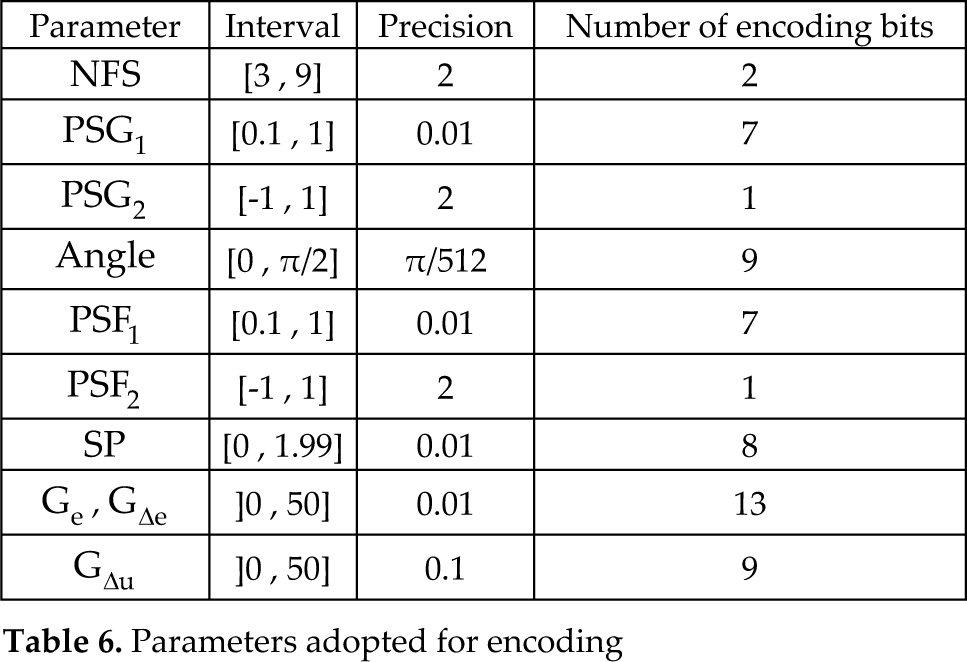
After many tests, we have adopted the parameter encoding shown in Table 6.
Parameters adopted for encoding
Many series of executions have been performed with variation of all the GA parameters (mainly the population size, the selection routine, the crossover method, the crossover and the mutation probabilities).
The best result has been obtained for Of = 17.7158 (DITAE = 0.05644). The corresponding GA characteristics are illustrated in Table 7. The progress of the GA that found the best fitness is presented in Fig. 16.

Progress of GA for the best fitness
GA adopted parameters

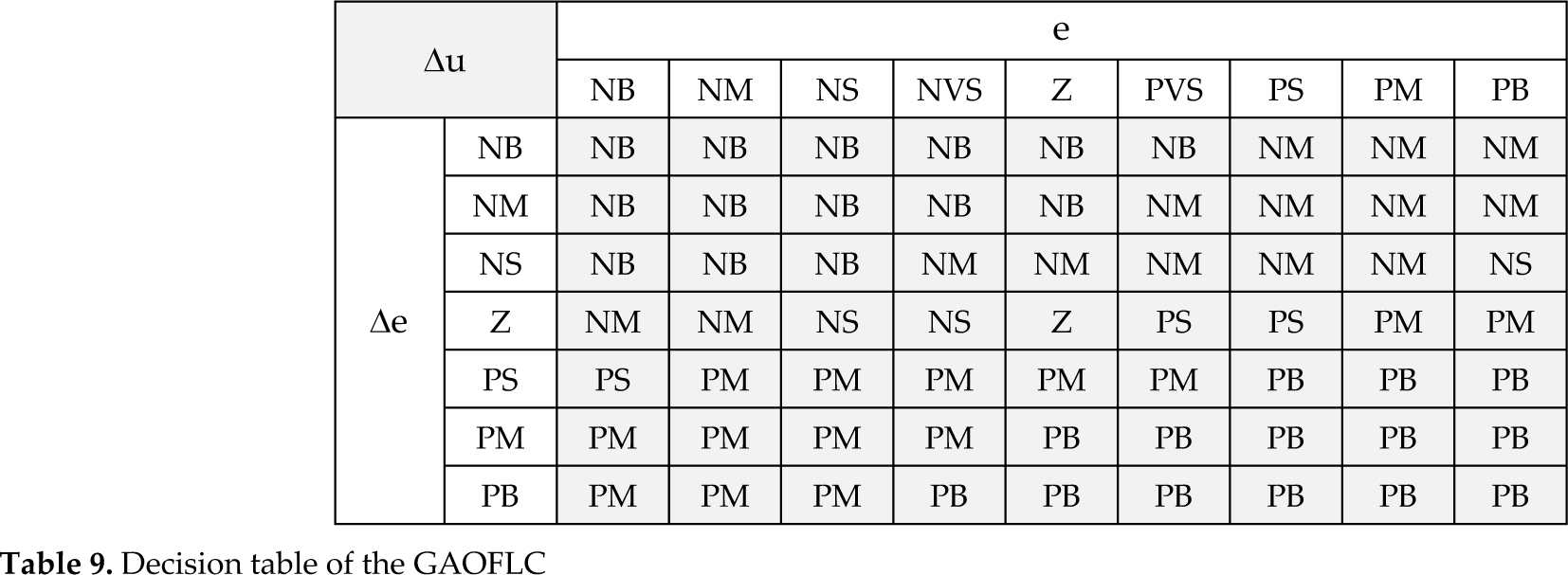
The optimal GAOFLC design parameters and the main characteristics (MFs and decision table) are shown in Table 8, Fig. 17 and Table 9.

Membership functions of the GAOFLC
GAOFLC design parameters

Decision table of the GAOFLC
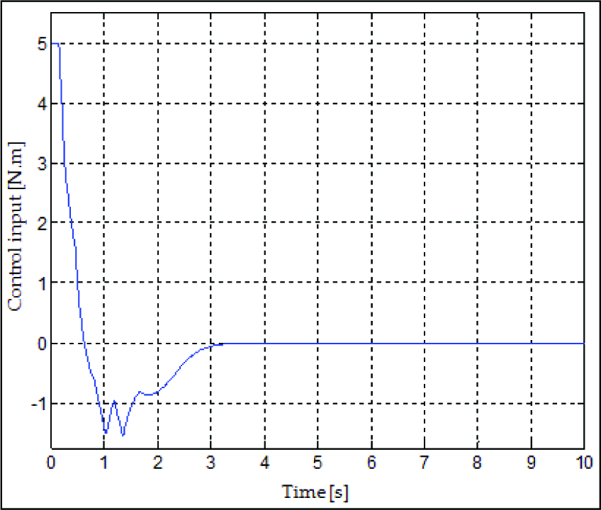
The obtained system response and the corresponding control input are shown, respectively, in Fig. 18 and Fig. 19. As can be seen from Fig. 18, the GAOFLC exhibits high precision and better step response performance in terms of rise time and settling time than the MPDFLC. Indeed, the reference is reached in less than two seconds with no undershoot or overshoot. We also observe that no residual vibration occurs upon arrival at the desired end-point. To test the GAOFLC capabilities in terms of robustness, we propose to simulate the lightweight robotic manipulator facing sudden payload variations at t = 0.5s. Four cases of payload reduction are considered: (a) 10%, (b) 30%, (c) 50%, (d) 70%. The corresponding responses are illustrated in Fig. 20.

GAOFLC-based end-point angular position response

GAOFLC-based generated control input

GAOFLC-based end-point angular position responses for the payload variation tests
We can observe that the performances are quite satisfactory even when the manipulator has lost 70% of its nominal payload.
The simulation results attest to the effectiveness and the robustness of the adopted control strategy.
6. Conclusion
This paper has been devoted to a study of advanced control schemes based on fuzzy logic concepts and genetic algorithm optimization applied to the end-point positioning of a planar one-link elastic robot arm: a Mamdani's PD fuzzy logic controller (MPDFLC) and a genetically optimized fuzzy logic controller (GAOFLC). The Timoshenko beam theory (TBT) concepts have been used in the comprehensive dynamic modelling of the considered lightweight robot manipulator. Two important damping mechanisms, internal structural viscoelasticity effect (Kelvin-Voigt damping) and external viscous air damping, have been included in addition to the classic effects of shearing and rotational inertia in the elastic link cross section. Then, an energetic deriving procedure based on the Lagrangian approach combined with the assumed modes method has been proposed to derive a suitable finite-dimensional dynamic model for the lightweight robot arm.
The first control scheme to be applied, i.e., the MPDFLC, has been designed in a long series of immensely time-consuming trial-and-error tests. The obtained best controller has given good performances in making the elastic manipulator tip angular position converge to the desired value with a fair response time, and in maintaining it at the reference without residual oscillations.
GAs being well known as powerful search tools that can reduce the time and effort involved in designing systems for which no systematic design procedure exists, they have been used to build an optimized FLC for our robotic control application. New contributions in the tuning procedures have been proposed. Explicitly, the innovations concern:
The technique of FS assignment to each of the grid nodes in the special case of equality of minimal distances between the points representing the candidate decision rules;
The formulation of the spacing law according to the spacing parameter in the decision rules table deriving method;
The formulations linking the trapezoidal and the two-sided Gaussian MFs;
The optimization and the diversification of the MF shapes offering possibilities of hybridization on the UD of each of the FLC input/output variables;
A simple solution to prevent important overlapping between the generated MFs.
The resulting GAOFLC has shown quite satisfactory performances in terms of fastness, stability and accuracy in end-point positioning of the lightweight manipulator arm. The synthesized intelligent controller has also shown robustness capabilities against disturbances caused by sudden load variations.
In future work, the mathematical model may be extended to a multiple elastic link robot arm structure. The joint elasticity, the gravity and the torsion effects may also be taken into account.
Further studies to improve the obtained performances through other advanced control schemes, as well as the use of other optimization techniques (such as ant colonies, swarm techniques, bio-inspired techniques, etc.), will be conducted.