Sage Journals: Discover world-class research

Abstract

The present paper a finite element implementation of a model of the arterial blood flow through the carotid artery with the effects of magnetic to considering fluid–wall interactions are investigated. The Navier–Stokes equations are used as the governing equations for the blood flow while an elastic compliant model is used for the arterial wall. The reduced one dimensional model solves the momentum and continuity equations in compliant tubes so as to reproduce the propagation of the pressure pulse in the arterial model. The obtained results adequately reproduce the general flow patterns reported in the literature. The results obtained in the investigation are in reasonably good agreement with experimental findings existing in the literature. The effects of a magnetic field have been used to control the flow, which may be useful in certain hypertension cases, etc.

Keywords

Blood flow elastic compliant model finite element method carotid artery model Hartmann number

1. Introduction

One of the leading causes of deaths in the world is due to heart related diseases. The heart diseases mainly occur due to temporary deficiency of oxygen or blood supply to the heart. This deficiency may be due to a constriction or obstruction in the blood supply to that part; the constriction involves the deposition of some fatty substances like cholesterol, cellular waste product, calcium, etc. Boesiger st al. [6] used magnetic resonance imaging (MRI) to study arterial homodynamics. This stenosis disturbs the flow of blood from its normal state which leads to the development of atherosclerosis. The atherosclerosis may cause the heart attack. Hemodynamic simulation studies have been frequently used to gain a better understanding of functional, diagnostic and therapeutic aspects of blood flow. These simulations employed compartmental representations or branching tube models of arterial trees as their geometrical substrate [1],[24][26], as well as localized multidimensional models have been often implemented to study arterial flow in more fine, detailed aspects. The study of the flow in the carotid artery bifurcation is of great clinical interest with respect to both, the genesis and the diagnostics of atherosclerotic diseases. It is well-known that the flow separation zone of the carotid sinus has the propensity to develop atherosclerotic plaques. In this sense, the local haemodynamic structure is intimately related to atherogenesis onset and progress [2]. Consequently, a more deep understanding and better descriptions of the flow structure in that region would be of greatest importance to the early detection of stenoses. Low shear stress regions are associated with the development of stenotics plaques. Despite the importance of chemical and physiological factors, the localized atherosclerotic lesions must be related to the local flow conditions as the other factor may be considered in a well mixed condition, i.e., uniformly distributed along the vessels. Several local three-dimensional (3D) in-vitro and computational flow models have been implemented, revealing the complex flow structure in the sinus district. Bharadvaj et. al.[28][29], defined a standard geometry of the carotid bifurcation (an average over 57 actual geometries from different subjects) and conducted stationary studies of the internal carotid blood flow. They found a region of low velocities near the non-dividing wall that extend with increasing Reynolds number, correspondingly, the opposite region showed large axial velocities and shear stresses, results that were confirmed by Rindt et. al[4], using experimental and computational stationary models. Ku and Giddens[5][7] observed a similar process in 3D models during the accelerating period of the diastole and the existence of velocities disturbances during the decelerating phase and at the onset of the diastole. Some similar experiments have been conducted in compliant models [14],[3]. To conduct focused numerical and in vitro realistic experiments of such a district as the carotid bifurcation, special attention must be paid to the boundary conditions applied to the model. As the pressure differences between inlet and outlet boundaries are only a small percentage of the systolic-diastolic pulse amplitude, this impose the problem of accurately determine the pressure, a condition that is often impossible to reach in practice. In this way, small errors in the imposed pressure could lead to great departure of the velocities from the real values. Conversely, if the flow is imposed as boundary conditions, negligible variations on these values could conduct to exaggerated low o high pressures in the analyzed segment. Accurate enough measures of those variables are very difficult or very costly to obtain simultaneously at the inflow and outflow regions for the entire cardiac period, even more in a noninvasive manner. This in turn, leads to implement models of the whole arterial tree in order to avoid artificial boundaries in the vicinity of the analyzed zone To conduct focused numerical and in vitro realistic experiments of such a district as the carotid bifurcation, special attention must be paid to the boundary conditions applied to the model. As the pressure differences between inlet and outlet boundaries are only a small percentage of the systolic-diastolic pulse amplitude, this impose the problem of accurately determine the pressure, a condition that is often impossible to reach in practice. In this way, small errors in the imposed pressure could lead to great departure of the velocities from the real values. Conversely, if the flow is imposed as boundary conditions, negligible variations on these values could conduct to exaggerated low o high pressures in the analyzed segment. Accurate enough measures of those variables are very difficult or very costly to obtain simultaneously at the inflow and outflow regions for the entire cardiac period, even more in a noninvasive manner. This in turn, leads to implement models of the whole arterial tree in order to avoid artificial boundaries in the vicinity of the analyzed zone. Recently, the coupling and integration of models with different dimensionality have been analyzed by Quarteroni et al.[16][21] linking together lumped models with 3D models of the arterial tree. The authors of the present work has proposed an alternative approach to coupling models of non-matching dimensionality and used them to implement a model of stenoses in the common carotid [12]. Here we implement a 3D finite element model of the carotid bifurcation on a standard geometry as proposed in [28][29] coupled with a 1D model of the rest of the arterial tree. Sharma et al. [13] made a mathematical analysis of blood flow through arteries using finite element Galerkin approaches. Sharma et al. [17] studied a MHD flow in stenosed artery using finite difference technique. A multiphase kinetic theory for the computation of viscosity of red blood cells and their migration from vessel walls has been discussed by Huang et al. [19]. In the above mentioned studies, no attempt has been made to study the effect of magnetic field on stenosis under porous medium together Gupta [18]. Kumar and Saket [20] investigated reliability of convective diffusion process in stenosis blood vessels. Nikparto and Firoozabadi [23] studied numerical study on effects of Newtonian and Non-newtonian blood flow on local hemodynamics in a multi-layer carotid artery Bifurcation.

2. Mathematical Model

2.1 Governing equations

In the present investigation we assume a complete model of the arterial tree have been developed with a three-dimensional model of the carotid bifurcation embedded in a reduced one dimensional Navier-Stokes equations considering compliant arterial walls for the rest of the arterial tree. The governing equations for the one dimensional portion of the model result in the following set of nonlinear hyperbolic equations

\frac{\partial Q}{\partial t} + \frac{\partial}{\partial x} (α \frac{Q^{2}}{A}) = - \frac{A}{ρ} \frac{\partial P}{\partial x} - \frac{π D}{ρ} τ_{0} - M Q

(1)

\frac{\partial A}{\partial t} + \frac{\partial Q}{\partial x} = 0

(2)

With α = \frac{A \int (u^{2} d A)}{Q^{2}}; τ_{0} = f_{r} \frac{ρ \tilde{u} | \tilde{u} |}{8}; Q = \tilde{u} A,

(3)

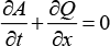
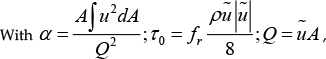
where A is the artery cross sectional area, u the axial velocity (ũ) the corresponding mean value); x the axial coordinate, P the mean pressure, ρ the blood density, Δ²Δx = 0, τ₀ the viscous shear stress acting on the arterial wall with fr a Darcy friction factor (in this work a fully developed parabolic velocity profile is considered). A closure equation is implemented relating the pressure to the cross sectional area:

P = P_{0} + E \frac{h_{0}}{R_{0}} {\sqrt{\frac{A}{A_{0}}} - 1}

(4)

A linear relationship between P and R is considered, being R de radius, E an effective Young modulus, h the thickness of the arterial wall and the subscript “o” denotes quantities evaluated at the reference pressure Po.

The former system of partial differential equations is discretized using a Galerkin's Least-Squares method for the normal equations of the hyperbolic system [12].

The local three dimensional fluid dynamics has described using the three dimensional time-dependent Navier-Stokes equations for incompressible Newtonian fluids where an Alternating Linear Euler method was implemented in order to take into account deformability of the domain as the arterial walls were considered as compliant tubes:

ρ \frac{\partial u}{\partial t} + ρ (u - v) \cdot \nabla u - μ \nabla^{2} u + \nabla P + M = f

(5)

div u =0

Δ^{2} Δ x = 0

(6)

where u is the fluid velocity, v is the moving reference frame velocity consistent with the

Alternating Linear Euler formulation, p is the pressure; Δ × is the displacement vector of the moving domain from its reference configuration ρ and μ stand for the constant fluid density and the dynamic viscosity, respectively.

\begin{array}{l} Δ x = δ n; u = \frac{d δ}{d t} n δ n \\ Δ x = δ n; u = \frac{d δ}{d t} n \end{array}

(7)

where δn is the displacement of the arterial wall in the normal direction of the surface ( n is the unit normal to the surface) The first of Eq. (7) is analogous to that of the one dimensional model given in Eq. (4) Another group of equations must be considered to appropriately set the coupling between the one dimensional and the three dimensional models at the interface surfaces. The continuity of mass, momentum and tractions must be imposed. For the Reynolds numbers prevailing at the carotid artery, continuity on tractions may be replaced by continuity on pressure. Consequently, continuity of blood flow is enforced at the interfaces between one dimensional and three dimensional zones jointly with weak continuity of pressures as described [12].

2.2 Numerical Method

For the numerical solution of the three dimensional flow problem the finite element method was applied: the approximation makes use of P1-P1 bubble tetrahedral elements with linear enriched interpolation functions for the velocity vector field and linear pressure[15]

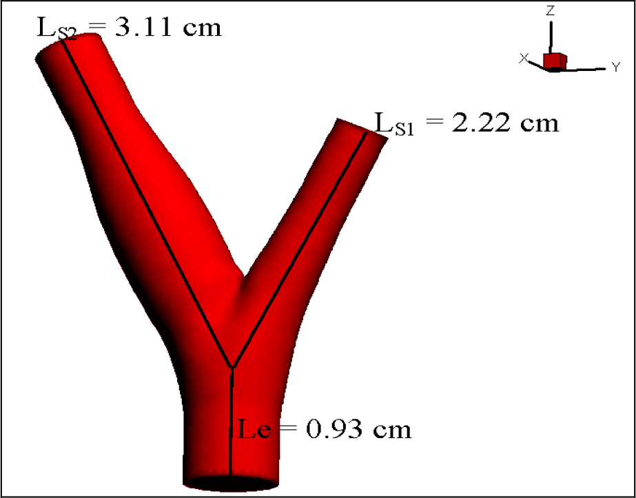
The equations are solved using the finite element SUPG (Standard Upwind-Petrov Galearkin) method with implicit Euler backward differences for the time derivatives and Picard iteration for the non-linear convection terms. The solution of the time-dependent three dimensional Navier-Stokes equations is performed in two sub-steps: in the first one, the bubble degrees of freedom are eliminated by direct substitution, and in the second one, those unknowns are updated as necessary for the evaluation of the second member of the set of equations at the following time step. The deformation of the domain is accounted through a Laplace equation for the displacement of the mesh –again, tetrahedral linear elements are used- where the boundary displacements at the arterial wall are given by the first of Eq. (7). Flow velocity patterns were calculated for an anatomically inspired carotid artery bifurcation model [27][28] as shown in Figure 1, the three dimensional mesh exposed in Figure 2 has 14159 nodes and 71732 tetrahedral elements.

Figure 1.

Three Dimensional Carotid Bifurcation of Geometry Model

Figure 2.

Three Dimensional of Finite Element Method mesh – Tetrahedral elements

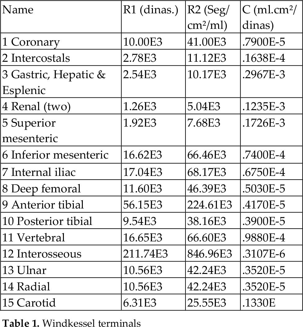
The one-dimensional model was described in Urquiza[12] discretized with a mesh displaying 686 nodes with three degrees of freedom (A, P, Q) per node and 642 elements. The inlet boundary condition describing the heart input flow was obtained from ^[22] and has a period T=0.8sec. The model is complemented with lumped “Windkessel” representations of the peripheral beds. The geometry and other parameters involved are shown in Figure 3.

Table 1.

Windkessel terminals

Name	R1 (dinas.)	R2 (Seg/cm²/ml)	C (ml.cm²/dinas)
1 Coronary	10.00E3	41.00E3	.7900E-5
2 Intercostals	2.78E3	11.12E3	.1638E-4
3 Gastric, Hepatic & Esplenic	2.54E3	10.17E3	.2967E-3
4 Renal (two)	1.26E3	5.04E3	.1235E-3
5 Superior mesenteric	1.92E3	7.68E3	.1726E-3
6 Inferior mesenteric	16.62E3	66.46E3	.7400E-4
7 Internal iliac	17.04E3	68.17E3	.6750E-4
8 Deep femoral	11.60E3	46.39E3	.5030E-5
9 Anterior tibial	56.15E3	224.61E3	.4170E-5
10 Posterior tibial	9.54E3	38.16E3	.3900E-5
11 Vertebral	16.65E3	66.60E3	.9880E-4
12 Interosseous	211.74E3	846.96E3	.3107E-6
13 Ulnar	10.56E3	42.24E3	.3520E-5
14 Radial	10.56E3	42.24E3	.3520E-5
15 Carotid	6.31E3	25.55E3	.1330E

Figure 3.

Volume difference between systole and diastole.

The whole model was computationally implemented in a numerical framework[11] that allows to easily integrate different kinds of elements as “plug and play” without modifying the main program, i.e., the programmer only must to provide the elemental matrices and to organize the input in such a way that all run together. The systems of algebraic equations are solved by Gauss –Siedal mehod.

Table 2.

Geometrical and Rheological values of Arterial Segments.

Name	Length (cm)	Proximal radius (cm)	Distal radius (cm)	E × h (dinas/cm)
1 Ascending aorta A	1.0	1.46	1.46	741500
2 Ascending aorta B	3.0	1.45	1.45	741500
3 Aortic arch A	2.0	1.12	1.12	741500
4 Aortic arch B	3.9	1.07	1.07	576200
5 Thoracic aorta A	5.2	1.0	1.0	545640
6 Thoracic aorta B	10.4	0.675	0.675	394000
7 Abdominal aorta A	5.3	0.61	0.61	370500
8 Abdominal aorta B&C	2.0	0.6	0.6	348000
9 Abdominal aorta D	10.6	0.58	0.58	352400
10 Abdominal aorta E	1.0	0.52	0.52	252500
11,31 Common iliac	5.8	0.37	0.37	368150
12,32 External iliac	14.4	0.32	0.32	148700
13,33 Femoral	44.3	0.26	0.26	230900
14,34 Posterior tibial	33.1	0.25	0.25	667500
15 Innominate	3.4	0.62	0.62	377000
16,17 Subclavian A	3.4	0.423	0.423	288700
18,19 Subclavian B	42.2	0.403	0.403	1170000
20,21 Ulnar A	6.7	0.215	0.215	679100
22,23 Ulnar B	17.1	0.203	0.203	717664
24,25 Carotid	20.8	0.37	0.37	264000
26,27 External carotid	17.7	0.177	0.177	259000
28,35 Anterior tibial	34.3	0.13	0.13	513145
29,30 Radial	23.5	0.174	0.174	682580

3 Results

Here we present some illustrative plots at selected times. In general, the flow has a very complex and unsteady structure showing an early back flow due to the inversion of the pressure gradient at the peak of the systole (Figure 4). A considerable deformation of the artery volume can be observed in Figure 3 where volume differences during diastole (red shaded) and systole (black wire frame) are displayed.

Figure 4.

Normal Stress during systole at t = 5.0E-2 sec. -Inverse pressure gradient

As can be seen in Figure 5 a zone of low velocities near the non-divider wall of the carotid sin sinus is observed and contrariwise, a high velocity region is displayed near the divider wall. These results are in well agreement with those obtained experimentally and numerically in references [8][28][29][14]. Detailed inspection of the computational results displays the general characteristics occurring in the carotid sinus, a period with reverse axial flow starts at the peak systole and remains until the beginning of diastole.

Figure 5.

Velocity profile during systole

4. Conclusions

A mathematical model that face the problem of simulating compliant three dimensional arterial districts coupled with a one dimensional model of the rest of the arterial tree has investigated. The resulting scheme has shown excellent capabilities to deal with considerable domain deformations while preserving the computational efficiency. The numerical results of the blood flow field for the carotid artery with magnetic effect are in general good agreement with those reported previously in the literature for both experimental and numerical cases. Our investigation may be helpful for the medical practitioners and Bio-mathematicians to understand the flow of blood in the presence of magnetic effects. The results are interpreted in the context of blood in the carotid arteries keeping the magnetic effects in view. The outcomes of investigation done may be useful for the treatment of hypertension patients through magnetic therapy.

References

Bruinsma

Arts

Dankelman

Spaan

J.A.E.

: Model of the coronary circulation based on pressure dependence of coronary resistance and compliance, Basic Res. Cardiol. 83 (1988) 510–524.

Caro

C.G.

Fitzgerald

J.M.

Schroter

R.C.

: Atheroma and arterial wall observations, correlation and proposal of a shear dependent mass transfer mechanism for atherogenesis, Proc. R. Soc. London, B177, 109–159, 1971.

Gijsen

F.J.H.

: Analysis of the axial flow fields in stenosed carotid artery bifurcation models: LDA experiments, J. Biomechanics, Vol. 29, pp 1483–1489, 1996.

Rindt

C.C.M.

Steenhoven

A.A.

van Janssen

J.D.

Reneman

R.S.

Segal

: A numerical analysis of steady flow in a three-dimensional model of the carotid artery bifurcation, Journal of Biomechanics, Vol. 23, pp 461–473, 1990.

D.N.

Giddens

D.P.

Hemodynamics of the normal carotid bifurcation. Ultrasound in Medicine and Biology 11 (1), 13–26, 1985.

Boesiger

Maier

S.E.

Kecheng

Scheidegger

M.B.

Meier

, Visualisation and quantification of the human blood flow by magnetic resonance imaging, J. of Biomechanics 25, 55–67, (1992).

D.N.

Giddens

D.P.

Zarins

C.K.

Glagov

: Pulsatile flow and atherosclerosis in the human carotid bifurcation. Arteriosclerosis 5 (3), 293–302, 1985.

Rene

Botnar H

Rappitsch

Scheidegger

M.B.

Liepsch

Perktold

Boesiger

: Hemodynamics in the carotid artery bifurcation: A comparison between numerical simulations and in vitro MRI measurements, Journal of Biomechanics 33, 137–144, 2000.

Sonneveld

: Multigrid and Conjugate Gradient Methods as Convergence Acceleration Techniques”, in “Multigrid Methods for Integral and Differential Equations”, Clarendon Press, Oxford, 1985.

10.

Yuocef

Saad

, SPARSEKIT: A basic tool kit for sparse matrix computation, University of Illinois,.

11.

Urquiza

S.A.

Venere

M. J.

“An Application Framework Architecture For Fem And Other Related Solvers”, pp. 3099–3109, ISSN 1666-6070, MECANICA COMPUTACIONAL Vol. XXI, Idelsohn

Sonzogni

Cardona

Eds., CERIDE, Sta Fe, 2002.

12.

Urquiza

Reutemann

Vénere

Feijoo

: Acoplamiento de Modelos Unidimensionales y Multidimensionales para la Resolución de Problemas Hemodinámicos”, ENIEF2001, XII Congress on Numerical Methods and their Applications, October 31 – November 2, 2001, Córdoba – Argentina.

13.

Sharma

G.C.

Jain

Kumar

, Finite element Galerkin approach for a computational study of arterial flow, Applied Mathematics and Mechanics 22 (9), 1012–1018, (September 2001).

14.

Anayiotos

A.S.

Jones

S.A.

Giddens Glagov

Zarins

C.K.

: Shear Stress at a Compliant Model of the Human Carotid Bifurcation, J. Biomech. Engng, V117, 98–106, 1994.

15.

Pironneau

: Finite-element methods for fluids, Wiley, New York, 1989.

16.

Quarteroni: Modeling the cardiovascular system: A mathematical challenge, Mathematics Unlimited – 2001 and Beyond, Engquist

Schmid

Eds, 961972, Springer-Verlag, 2001.

17.

Sharma

G.C.

Jain

Kumar Anil (2001): MHD flow in stenosed artery, Proceedings in International Conference on Mathematical Modeling, January 29–31, I.I.T. Roorkee, 683–687.

18.

Gupta Kumar

Anil

(2009): Finite element Galerkin's scheme for flow in blood vessels with magnetic effects, Int. J. applied systemic studies, vol.3(2), 283–293.

19.

Huang

Lyczkowski

R. W.

Gidaspow

(2009): Pulsatile flow in a coronary artery using multiphase kinetic theory, J. Biomech., Vol. 42, No. 6, pp. 743–754.

20.

Kumar

Anil

Saket

R K

: Reliability of Convective Diffusion Process in Stenosis Blood Vessels, Chemical product and process modeling, vol.3(1), article 25, 2008.

21.

Formaggia

Nobile

Quarteroni

Veneziani

: Multiscale Modelling of the Circulatory System: A Preliminary Analysis, Comput. Visual. Sci., 1999, vol 2 issue 2/3, pag. 75–83.

22.

Stettler

J.C.

Niederer

Anliker

: Theoretical Analysis of arterial hemodynamics including the influence of bifurcations”, Annals of Biomedical Engineering, 45–56, 1980.

23.

Nikparto

Ali

Bahar

Firoozabadi Numerical study on effects of Newtonian and Non-newtonian blood flow on local hemodynamics in a multi-layer carotid artery Bifurcation, Computer Methods in Mechanics, 11–23, 2011.

24.

Kumar

Anil

Varshney

C L

Lal

: Crank-Nicolson scheme to transient MHD free convective flow through semi-infinite vertical porous plate with constant suction and temperature dependent heat source, Proceedings of the International Conference on Advances in Computing and Artificial Intelligence, ACM DL, pp 85–91. 2011.

25.

Avolio

. Multi-branched model of the human arterial system. Med. Biol. Eng. Comp. 1980, 18: 709–718.

26.

Schaaf

Abbrecht

. Digital Computer Simulation of Human Systemic Arterial Pulse Wave Transmission: A Nonlinear Model. J. Biomechanics Engineering. 1972, 5: 345–364.

27.

Bharadvaj

B,K.

Mabon

R.F.

Giddens

D.P.

: Steady flow in a model of the human carotid bifurcation-I. Flow Visualization, Journal of Biomechanics, 15,349–362, 1982.

28.

Bharadvaj

B. K.

Mabon

R.F.

Giddens

D.P.

: Steady flow in a model of the human carotid bifurcation-I. Laser-Doppler anemometer measurements, J. Biomechanics, 15,363–378, 1982.

Performance and Analysis of Blood Flow through Carotid Artery

Abstract

Keywords

1. Introduction

2. Mathematical Model

2.1 Governing equations

2.2 Numerical Method

3 Results

4. Conclusions

References