Sage Journals: Discover world-class research

Abstract

In this study, we demonstrate the usefulness of ARIMA-Intervention time series analysis as both an analytical and forecast tool. The data base for this study is from the PACAP-CCER China Database developed by the Pacific-Basin Capital Markets (PACAP) Research Center at the University of Rhode Island (USA) and the SINOFIN Information Service Inc, affiliated with the China Center for Economic Research (CCER) of Peking University (China). These data are recent and not fully explored in any published study. The forecasting analysis indicates the usefulness of the developed model in explaining the rapid decline in the values of the price index of Shanghai A shares during the world economic debacle stating in China in 2008. Explanation of the fit of the model is described using the latest development in statistical validation methods. We note that the use of a simpler technique although parsimonious will not explain the variation properly in predicting daily Chinese stock prices. Furthermore, we infer that the daily stock price index contains an autoregressive component; hence, one can predict stock returns.

Keywords

ARIMA Intervention Analysis Forecasting Chinese Stock Prices

1. Introduction

In this study, we report an analysis not heretofore reported in the literature and for the data base collected. Our purpose is twofold; (1) to analyze data by implementing ARIMA-Intervention analysis (Box and Tiao, 1975); and to assess the prediction and forecasting of Chinese stock market prices over a lengthy enough period of time where stock prices fluctuated during varying temporal economic movements. We study the Chinese equity markets to understand the predictable properties in this fast growing but volatile market. Previous studies of the Chinese equity markets include Jarrett, Pan and Chen (2009) who studied the relationship between the Macroeconomy of China as it relates to the equity markets of Shanghai and Shenzhen. In addition, Thomas (2001) discussed in detail the workings of the Shanghai equity market over its illustrious history offering insights into the characteristics of the equity markets. His study included the behavior of both domestic and foreign investors in four equity markets. The history discussed is of the twentieth century and not the twenty-first century. Others (Eun and Huang, 2007; Ng and Wu, 2007; Shenoy and Ying, 2007, Weili et al. , 2009, Wang et al. , 2004 and Wang et al. , 2007) investigated the rapid growth in the Chinese equity markets and why they became increasing important for investors in global markets. In addition, Bailey, Cai, Cheung and Wang (2006) studied the Shanghai Equity Market and discovered some characteristics concerning order balances of individuals, and institutional investors. Our purpose, here, is to investigate the Chinese equity markets to explain and discover if certain anomalies noted in more developed equity markets are present or not in the Chinese markets.

Following the study of Zhong, Gui and Lui (1999) for the Chinese Bourses (Shanghai and Shenzhen), we selected a newer and finer data base from the PACAP-CCER China Database developed by the Pacific-Basin Capital Markets (PACAP) Research Center at the University of Rhode Island (USA) and the SINOFIN Information Service Inc, affiliated with the China Center for Economic Research (CCER) of Peking University (China). The length of data was for approximately ten years resulting in a time period where analysis can lead to interpretable results. Smaller time periods such as two or three or even four years are usually too small to reduce the effects of disturbances in economic data and more specifically do not produce enough degrees of freedom such that one may identify significant events and factors. A small number of degrees of freedom in sample data may not lead to determining “statistically significant” events even when they exist. The theoretical minimum number of observations for an ARIMA model is p+q+d+1, with the caveat that observations below three result in infinite standard errors. We also require each parameter in a regression equation to have at least one observation (Hyndman and Kostenko, 2007). That would result in a minimum number of observations for our model of five (one for the AR term, one for the difference of price, one for the IV volume, and two for the dummy variable intervention). To further account for randomness in the data we increased the sample size knowing that margins of error decrease proportional to the square of the sample size. [See Hyndman and Kostenko (2007)].

The regression will include for the response variable is the daily price index for the entire data base on daily returns produce by the PACAP-CCER Greater China Database. These data are part of the website created for research on Pacific-Basin nations. [The website and its content is a copyright of PACAP-CCER. All rights reserved. If you have any question or comment, please e.mail to chinadat@etal.uri.edu.]. The data base contains information from 01/1990 to 12/2009. The length of time is long enough for serious investigation which produce results that is not highly influenced by business cycles but long enough for us to create a useful ARIMA-Intervention model for forecasting.

2. ARIMA Modeling and Intervention Analysis

We follow the methods of stochastic time-series ARIMA modeling to analyze and find a model for prediction of changes, variation sand interruptions (interventions) in the movement of stock prices for China over time. ARIMA modeling with intervention may help analysts understand whether economic events such as a “global financial crisis” have impact on the change in Chinese stock prices if it exists (Shanghai A-share simple arithmetic mean index). This will provides information for financial analysts, economic forecasters and decision-makers to plan for and cope with sudden movements in the prices of Chinese stock. Previously, the application of ARIMA modeling with and without intervention was implemented in such applications as system scheduling and simulation (Ip, 1997; Ip et al., 1999), tourism forecasting (Du Preez and Witt, 2003, and Cho 2001) investigation and forecast of economic factors (Chung et al., 2008) the financial crisis in China's Manufacturing (Chung et al., 2009) demand in telemarketing centers (Bianchi, Jarrett and Hanumara, 1998) and the impact analysis on air travel demand (Lai and Lu, 2005).

As discussed before by Box and Tiao (1975) an intervention model is of the general form:

γ_{t} = V (B) I_{t} + N

(1)

where I_t is an intervention or dummy variable that is defined as I_t = 1, for t = T and I_t = 0 for t ≠ T.

In the transfer function models, the input is a general exogenous times series that influences the output series. We consider a special situation in which the input is a series of indicator variables that rrepresent the occurrence of identifiable unique events that affect the output variable. The identifiable events are the interventions. We now assume an intervention occurred, hence we ask the question whether evidence exists change in the time series of the type anticipated occurred. Furthermore, what is the estimated size fo this change? Intervention analysis model, introduced by Box and Tiao (1975), is the major work in this area. However, a great deal of the terminology is due to Glass (1972). [A formal example of its use is displayed in Brocklebank and Dickey (2003, pp. 143–237)].

To identify the correct model for prediction and explanation, ARIMA modeling consists of three steps. First, we identify the order of the differencing, i.e., d. This preliminary step is essential to produce a stationary time series model for identification. There are several solutions including the Augmented Dickey-Fuller (ADF) test and those following the Ljung and Box (1978) analysis. In this analysis, we chose both methods although each method produced the same results. Either method will yield the correct order of the left hand side variable (price). Second, one diagnoses and identifies the parameters autoregressive and moving-average portions of the ARIMA model, i.e., the p and q terms. p refers to the autoregressive component and q refers to the moving-average component of the model. The autocorrelation function (ACF), partial autocorrelation function (PACF) and the cross-autocorrelation function (CACF) are important to tentatively estimate the parameters of the model. In turn, statistical measures provide the evidence to support the determination of an appropriate model for estimation and prediction. Third, one diagnoses the residuals (noise). The Portmanteau Q-statistic is in turn permits one to judge the fit of the model to the data based on the ACF of the residuals. Based on the results of this three step procedure which diagnoses the data, we are led to choosing a lag of one to produce and stationary series. In turn, the examination of the various autocorrelation and partial autocorrelation functions; we are led to concluding that an autoregressive (AR) model having one term fits the data studied. We define the intervention as the present financial crises initially triggered in July, 2007 which spread first to Europe and then to China. Hence, data was assigned a value of 1 for the variable for I_t [an intervention, the variable denoted by inter], beginning July 2007 and 0 before the intervention period. For V (volume), the data is the volumes of transactions corresponding to the daily price index. [Autocorrelations and Q statistics can be acquired from the author at their address]

Alternatives to ARIMA do exist for forecasting stock prices. For example, neural networks popularized in recent years due to increased availability of computer software are comparable to ordinary least squares regression (OLS) regression. However, neural networks are a black box method for providing accurate predictions, but contain little or no explanatory power. Hence, they are inappropriate for this study (see Lievano and Kyper, 2006). To analyze interrupted (intervention) series, sophisticated techniques like Fourier analysis and cross-spectrum analysis are available (see Hill and Lewicki, 2007). However, these techniques are more appropriate for complex time series with cyclical components or the simultaneous analysis of two series respectively, and were not deemed appropriate to test here.

3. The Analysis of the ARIMA Intervention Model

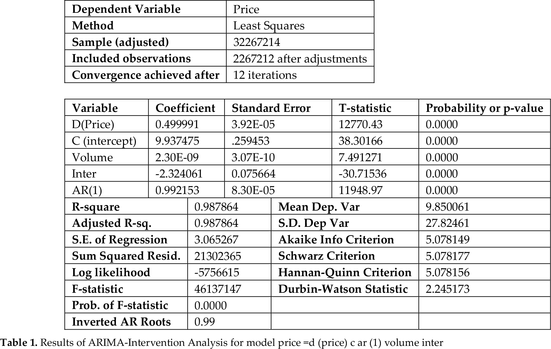
We include the financial crisis as the intervention of the time series which results in an ARIMA-Intervention model. As the global financial crisis extended to China in September 2008 and beyond, the intervention was initiated at that time. In the Appendix Table 1, we have the results in tabular form for both the model estimates and the initial T-statistics for the model. Note, the coefficients have T-statistics largely different from zero with p-values of 0.0000. This indicates that all the estimated coefficients are nonzero. One way to write the equation of the model is as follows:

Table 1.

Results of ARIMA-Intervention Analysis for model price = d (price) c ar (1) volume inter

Dependent Variable	Price
Method	Least Squares
Sample (adjusted)	32267214
Included observations	2267212 after adjustments
Convergence achieved after	12 iterations

Variable	Coefficient	Standard Error	T-statistic	Probability or p-value
D(Price)	0.499991	3.92E-05	12770.43	0.0000
C (intercept)	9.937475	.259453	38.30166	0.0000
Volume	2.30E-09	3.07E-10	7.491271	0.0000
Inter	−2.324061	0.075664	−30.71536	0.0000
AR(1)	0.992153	8.30E-05	11948.97	0.0000

R-square	0.987864	Mean Dep. Var	9.850061
Adjusted R-sq.	0.987864	S.D. Dep Var	27.82461
S.E. of Regression	3.065267	Akaike Info Criterion	5.078149
Sum Squared Resid.	21302365	Schwarz Criterion	5.078177
Log likelihood	−5756615	Hannan-Quinn Criterion	5.078156
F-statistic	46137147	Durbin-Watson Statistic	2.245173
Prob. of F-statistic	0.0000
Inverted AR Roots	0.99

\begin{array}{l} γ_{t} = 9.9374475 + 0.499991 (Δ γ_{t}) + (2.30 E - 09) V_{t} - 2.324061 I_{t} + \\ 0.992153 γ_{t - 1} \end{array}

When we evaluate the differenced term, (Δ Y_t), the equation for the model becomes:

\begin{array}{l} 0.500009 γ_{t} = 9.937475 - 0.499991 γ_{t - 1} + (2.30 E - 09) V_{t} - \\ 2.324061 I_{t} + 0.992153 γ_{t - 1} \end{array}

Last, we evaluate the AR (1) term 0.992153 Y_t-1 to form the final estimation model:

\begin{array}{l} 0.500009 γ_{t} = 9.937475 + 0.492162 γ_{t - 1} + (2.30 E - 09) V_{t} - \\ 2.324061 I_{t} \end{array}

What we learn from the estimated model equation is that the intervention is significant and that prices were inversely related to financial crisis. This is what we would expect the results to be and is likely to be corroborated by studies using other methods for analyzing time series data having been related to the economics of the environment. Furthermore, the volume effect, although statistically significant, leads us to conclude that there is only a tiny effect on the volume of transaction on prices. The differencing which was necessary to build a time series that was stationary for modeling purposes was also significant and positive. Last, the significant autoregressive coefficient of the first order, i.e., AR (1), led to the estimated coefficient of 0.492162 for lagged value of Y_t, i.e., Y_t-1.

4. Additional Analytical Results

In addition the analytical table in the Appendix further gives diagnostic information about the estimated model and its equation. The coefficient of determination and the adjusted coefficient of determination are both extremely large and are the same because of the large number of degrees of freedom, i.e., 0.987864. The standard error of regresion (3.065267) is relatively small. The log likelihood statistic is −5756615 and is the ingredient in likelihood ratio tests. A likelihood ratio test is used to compare the fit of two models one of which is nested within the other. Both models are fitted to the data and their log-likelihood recorded. A null hypothesis is often stated by saying the parameter θ is in a specified subset Θ₀ of the parameter space Θ. Higher values of the statistic mean that the observed outcome was more than or equally likely or nearly as likely to occur under the null hypothesis as compared to the alternate, and the null hypothesis cannot be rejected. Since our results indicate a very large value for the log likelihood, we cannot reject the the null hypothesis.

The F-statistic of 46137147 with a probability of 0.0000 indicates that the regression coefficients (except for the constant or intercept term) are nonzero. The probability (p-value) indicates the marginal significance of the F-test.

The AIC (Akaike information criterion, 1974) indicates the usefulness of model selection for non-nested alternative. Smaller values for AIC is preferred. As in our illustration, one best chooses the length of the lag distribution by choosing the lowest value of the AIC, 5.078149 is for our estimated model. The Schwarz criterion (1978) is 5.078156. It is an alternative to the AIC and penalizes more greatly for additional coefficients. The two criterions are so similar that either will lead to the conclusion that this model is best. Last, the Hannan-Quinn Criterion (1979) yields an additional test for model selection similar to the other two noted before. The result is again very similar to the AIC and Schwarz criterions already considered.

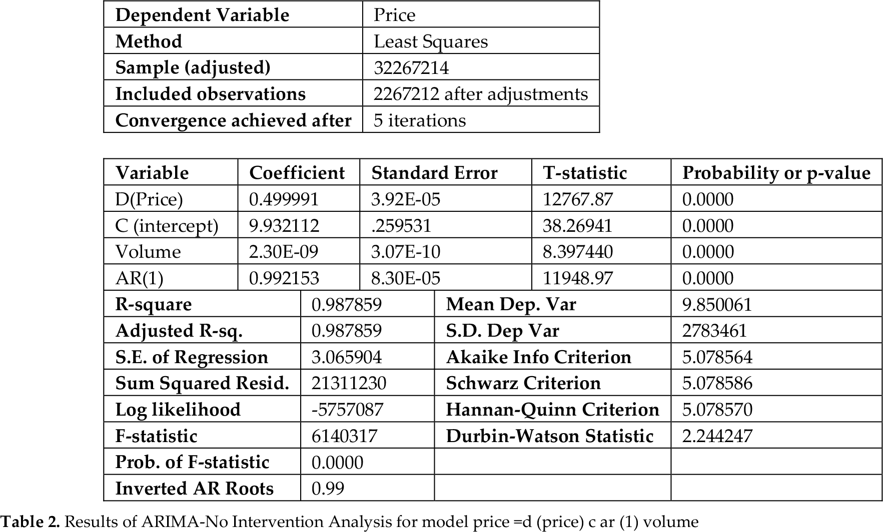
The well-known Durbin-Watson Statistic is the most universally accepted testing criterion for measuring the magnitude of autocorrelation in the residuals from a model. A statistic of 2.245173 would lead one to conclude that one should accept the hypothesis of the autocorrelation coefficient equal zero. With the absence of autocorrelation in the residuals from forecast, one concludes the previous tests of significance are useful and the model is available for predictive purposes. The Portmanteau Q-statistic calculated along with the autocorrelation function of the residual resulted in the same conclusion. Hence, the estimated model was a good fit for the time series. If we were to fit the model without the intervention the AIC, Schwarz Criterion and Hanna-Quinn Criterion would all have larger values indicating also that the model with the intervention was a better fit to the data. The coefficient of determination adjusted for degrees of freedom was also small for the model without intervention. To further examine these results observe Appendix Table 2 which contains the ARIMA model without use of the intervention term. Note, that in Appendix Table 2 we have the results of the analysis when the model does not contain the intervention term. Observe the three criterions Akaike, Schwarz and Hannan-Quinn produce values larger than existing for these criterions for the ARIMA model with intervention. Though these values appear small, these values are not so relatively small because the left hand size variable is D (PRICE). This variable has an extremely small standard error. The interpretation is obvious at this point that including the intervention term has benefits.

Table 2.

Results of ARIMA-No Intervention Analysis for model price = d (price) c ar (1) volume

Dependent Variable	Price
Method	Least Squares
Sample (adjusted)	32267214
Included observations	2267212 after adjustments
Convergence achieved after	5 iterations

Variable	Coefficient	Standard Error	T-statistic	Probability or p-value
D(Price)	0.499991	3.92E-05	12767.87	0.0000
C (intercept)	9.932112	.259531	38.26941	0.0000
Volume	2.30E-09	3.07E-10	8.397440	0.0000
AR(1)	0.992153	8.30E-05	11948.97	0.0000

R-square	0.987859	Mean Dep. Var	9.850061
Adjusted R-sq.	0.987859	S.D. Dep Var	2783461
S.E. of Regression	3.065904	Akaike Info Criterion	5.078564
Sum Squared Resid.	21311230	Schwarz Criterion	5.078586
Log likelihood	−5757087	Hannan-Quinn Criterion	5.078570
F-statistic	6140317	Durbin-Watson Statistic	2.244247
Prob. of F-statistic	0.0000
Inverted AR Roots	0.99

5. Summary and Conclusions

The stock market price index in China was modeled by the methods of ARIMA-Intervention analysis and produced a fit for one to analyze and draw conclusion concerning how the index behave over time. The results indicate that the World Financial Crisis included China and affected its stock as well as its manufacturing industry. The intervention effect as measured in this study was alarming and clearly felt by the financial industry in China as well as its other component. The negative effect of the stock market decline is likely to correlate with the decline in Chinese manufacturing during the period and to have negative impacts on the Chinese Macroeconomy. In addition, the results corroborate that daily prices of Chinese equity securities have an autoregressive component. Whether this in a permanent or temporary component of the time series requires a more exhaustive study involving long term modeling of financial time series as exemplified by Ray, Jarrett and Chen (1997) in a study of the Japanese stock market index. One very basic conclusion is that we indicated that the use of intervention analysis is very useful in explaining the dynamics of the impact of serious interruptions in an economy and the changes in the time series of a price index in a precise and detailed manner.

References

Akaike

(1974) A new look at the statistical model identification. IEEE Transactions on Automatic Control 19 (6), 716–723.

Bailey

Cai

Cheung

Y.L.

Wang

F.F.

(2009) Stock returns, order imbalances and commonality: Evidence on individual, institutional, and proprietary investors in China,” Journal of Banking and Finance, 33, (1) 9–19.

Box

G.E.P.

Tiao

G.C.

(1975) Intervention analysis with applications to economic and environment problems, Journal of the American Statistical Association, 70 (349) 70–79.

Bianchi

Jarrett

J.E.

Hanumara

R.C.

(1998) An analysis of Forecasting for telemarketing centers, International Journal of Forecasting, 14 (4) 497–504.

Brocklebank

J.C.

Dickey

D.A.

(2003) SAS for Forecasting Time Series 2nd ed. Wiley: ISBN 0-47139566-8.

Du Preez

Witt

S.F.

(2003) Univariate versus multivariate time series forecasting: An application to international tourism demand, International Journal of Forecasting, 19 (3), 435–451.

Cho

(2001) Tourism forecasting and its relationship with leading economic indicators, Journal of Hospitality and Tourism Research, 25 (4), 399–420.

Chung

R.C.P.

W.H.

Chan

S.L.

(2008) Impacts of the overheating economy on China's manufacturing, The International Journal of Advanced Manufacturing Technology, DOI: 10.1007/s00170-008-1792-y ISSN: 02683768 (print) or 14333015 (online).

Chung

R.C.P.

W.H.

Chan

S.L.

(2009) An ARIMA-Intervention analysis model for the financial crisis in China's Manufacturing industry, International Journal of Engineering Business Management, 1 (1), 15–18.

10.

Eun

C.S.

Huang

(2007) Asset pricing in China's domestic stock markets: Is there logic? Pacific-Basin Finance Journal, 15 (5), 452–480.

11.

Glass

G.V.

(1972) Estimating the effects of intervention into a nonstationary time series, American Educational Research Journal, 9, 463–477.

12.

Hannan

E.J.

Quinn

B. G.

(1979) The Determination of the order of an auto regression, Journal of the Royal Statistical Society, B, 41, 190–195.

13.

Hill

Lewicki

(2007) STATISTICS: Methods and applications. StatSoft, Tulsa, OK.

14.

Hyndman

Kostenko

(2007) Minimum sample size requirements for seasonal forecasting models, Foresight 6, 12–15.

15.

W.H.

(1999) Rule Based ARIMA for FMS, Journal of Materials Processing Technology, 66(1–3), 240–243.

16.

W.H.

Fung

Keung

K.W.

(1999) An investigation of stochastic analysis of flexible manufacturing systems simulation, International Journal of Advanced Manufacturing Technology, 15, 244–250.

17.

Jarrett

J.E.

Pan

Chen

(2009) Do the Chinese bourses (stock markets) predict economic growth? International Journal of Business and Economics, 8 (3) 201–211.

18.

Lai

S.L.

W.L.

(2005) Impact analysis of September 11 on air travel demand in the USA, Journal of Air Transport Management, 11, 455–458.

19.

Lievano

R. J.

Kyper

E. S.

(2006) Data mining reliability: Model-building with MARS and neural networks. Advances in business and management forecasting, 4, 215–242.

20.

Ljung

G. M.

Box

G.E.P.

(1978) On a measure of a lack of fit in time series models, Biometrika 65, 297–303.

21.

(2007) The trading behavior of institutions and individuals in Chinese equity markets, Journal of Banking and Finance, 31 (9), 2695–2710.

22.

Ray

Jarrett

J.E.

Chen

(1997) Identifying permanent and temporary components in daily and monthly Japanese stock prices, Financial Engineering and Japanese Markets 4 (3) 233–256.

23.

Schwarz Gideon

(1978) Estimating the dimension of a model, Annals of Statistics 6 (2), 461–464.

24.

Shenoy

Ying

J.Z.

(2007) Order imbalance and stock returns: Evidence from China, Quarterly Review of Economics and Finance, 47, 637–650.

25.

Thomas

W.A.

(2001) Western Capitalism in China: A History of the Shanghai Stock Exchange, Aldershot: Ashgate.

26.

Wang

Burton

B.M.

Power

D.M.

(2004) Analysis of the overreaction effect in the Chinese stock market, Applied Economics Letters, 11 (7), 437–442.

27.

Wang

Yang

(2007) Does the stock market affect firm investment in.

28.

China? A price informativeness perspective, Journal of Banking and Finance, 33, 53–62.

29.

Weili

Xiaoming

Jijao

(2009) Anomalies and heterogeneity of China stock markets in the financial Crisis, 2009 International Conference on New Trends in Information and Service Science, 875–879.

30.

Zhong

R.S.

Lui

C.B.

(1999) The Empirical Statistical Analysis of Chinese Stock Markets, Beijing: China Financial and Political Economics Press.

ARIMA Modeling with Intervention to Forecast and Analyze Chinese Stock Prices

Abstract

Keywords

1. Introduction

2. ARIMA Modeling and Intervention Analysis

3. The Analysis of the ARIMA Intervention Model

4. Additional Analytical Results

5. Summary and Conclusions

References