Sage Journals: Discover world-class research

Abstract

Forecasting accuracy drives the performance of inventory management. This study is to investigate and compare different forecasting methods like Moving Average (MA) and Autoregressive Integrated Moving Average (ARIMA) with Neural Networks (NN) models as Feed-forward NN and Nonlinear Autoregressive network with eXogenous inputs (NARX). Data used to forecast is acquired from inventory database of Panasonic Refrigeration Devices Company located in Singapore. Results have shown that forecasting with NN offers better performance in comparison with traditional methods.

Keywords

ARIMA Forecasting Inventory Neural Networks Safety Stock

1. Introduction

Demand forecasting plays an important role in inventory planning. In order to achieve an efficient management of inventory, accurate forecasting has to be aimed first. Among all the techniques and methods to forecast, Neural Networks (NN) offers desirable solutions in terms of accuracy. The use of NN in forecasting can be described intuitively as follows. Suppose there exists certain amount of historical data which can be used to analyze the behavior of a particular system, and then such data can be employed to train a NN that correlates the system response with time or other system parameters. Even though this seems a simple method, many studies show that NN approach is able to provide a more accurate prediction than expert systems or statistical counterpart (Bacha. & Meyer, 1992).

2. Literature Review

Neural Networks is usually involved in forecasting lumpy demand, characterized by intervals in which there is no demand and periods with large variation of demand. Traditional time-series methods may not be able to capture the nonlinear pattern in data. NN modeling is a promising alternative to overcome these limitations. Neural networks can be applied to time series modeling without assuming a priori function forms of models. Many varieties of neural network techniques including Multilayer Feed-forward NN, Recurrent NN, Time delay NN and Nonlinear Autoregressive eXogenous NN have been proposed, investigated, and successfully applied to time series prediction and causal prediction as shown in Figure 1. (a) Multilayer Feedforward NN (Davey et al., 1999) is the most common NN used in causal forecasting, the flow of information is from the input layer to the output layer. (b) Recurrent NN (Bengio et al., 1993; Conner & Douglas, 1994) is basically a Feedforward NN with a recurrent loop, therefore the output signals are fed back to the input. (c)Time delay NN (Wan, 1993; Back & Wan, 1995) integrates time delay lines. (d) Nonlinear Autoregressive eXogenous NN (Menezes Jose et al., 2006; Lin et al., 2000; Siegelmann et al., 1997) is a combination of all above NN, and is applied successfully in time series forecasting as well as causal forecasting.

Fig. 1.

NN used in forecasting

The following researches adopted NN in their aim to forecast demand for spare parts, with very promising results.

Gutierrez et al., (2008) adopted the most widely used method, Multi-Layered Perceptron (MLP which is a particular case of FFNN), trained by a Back-Propagation algorithm (BP). They used three layers of MLP: the input layer for input variables, hidden layer with three neurons and output layer with just one neuron. The input neurons represent two variables: a) the demand at the end of the immediately preceding period and b) the number of periods separating the last two nonzero demand transactions as the end of immediately preceding period. The output node represents the predicted value of the demand for the current period.

Specht (1991) adopted a Generalized Regression NN (GRNN). This network does not require an iterative training procedure as in back propagation method. They used four layers: the input layer, pattern layer, summation layer and output layer.

The input variables for GRNN are: a) Demand at the end of the immediately preceding target period; b) Number of unit periods separating the last two nonzero demand transactions as the end of the immediately preceding target period; c) Number of consecutive periods with no demand transaction in the immediately preceding target period.

Amin-Naseri & Rostami Tabar (2008) proposed the use of Recurrent Neural Networks (RNN). The network is composed from four layers: an input layer, a hidden layer, a context layer and an output layer. They used in this study real data sets of 30 types of spare parts from Arak petrochemical company in Iran and three performance measures: Percentage Best (PB), Adjusted Mean Absolute Percentage Error (A-MAPE) and Mean Absolute Scaled Error (MASE).

Their results show that NN can be used with promising results in comparison with traditional forecasting methods, like Moving Average (MA) and Single Exponential Smoothing (SES).

Aburto & Weber (2007) combined two forecasting methods which are ARIMA and Neural Networks. Input neurons are divided into two types of variables: Binary variables (12 variables such as ex payment, holiday) and simple numerical representing past sales with lag k (k – depends on the time window used). The efficiency of the hybrid model is compared with traditional forecasting methods (naïve, seasonal naïve, and unconditional average), including a SARIMAX method and several NN. The performance of each model is determined using two error functions.

To sum up, this comparative review of the literature has shed light on NN which is capable of modeling any time series without assuming a priori function forms and degrees of nonlinearity of a series. The challenges of demand forecasting include non-stationary, nonlinearity, noise and limit quantity of data. Other important issues include prediction risk (Moody, 1994) generalization error estimates (Larson, 1992), Bayesian methods (Mackay, 1994) non-stationary time series modeling and incorporation of prior knowledge (Weigend, 1995). This paper studies the adoption of NN for time series forecasting in a case study in a company. The main tasks of applying NN to time series modeling include incorporating temporal information, selecting proper input variable, and balancing bias/variance trade-off of a model.

3. Methodology

Artificial Neural Network (ANN) is an information processing system that has been developed as generalizations of mathematical models of human neural biology (Figure 2). ANN is composed of nodes or units connected by directed links. Each link has a numeric weight (W is the weight matrix).

Fig. 2.

Mathematical model of the artificial neuron

Notice that in Figure 2 we have included a bias b with the purpose of setting the actual threshold of the activation function.

υ_{i} = \sum_{j = 1}^{d} w_{i j} x_{j}

o_{i} = γ (υ_{i}) = γ (\sum_{j = 1}^{d} w_{i j} x_{j})

w = [\begin{array}{l} w_{11} & w_{12} & w_{13} & w_{1 d} \\ w_{21} & w_{22} & w_{23} & w_{2 d} \\ w_{31} & w_{32} & w_{33} & w_{3 d} \\ w_{m 1} & w_{m 2} & w_{m 3} & w_{m d} \end{array}]

where γ is the activation function, x_j is the input neuron j, o_i is the output of the hidden neuron i, and W is the weight matrix. The NN learns by adjusting the weight matrix. Therefore the general process responsible for training the network is mainly composed of three steps:

Feed forward the input signals

Back propagate the error

Adjust the weights

Basic structure of a NN is depicted in Figure 3, the input data being fed up at the input layer and the output data being collected at the output layer.

Fig. 3.

Basic structure of a NN

Training the NN is divided into four steps:

Data selection - Data selection step restricts subsets of data from larger databases and different kinds of data sources. This phase involves sampling techniques, and database queries.

Data preprocessing – data preprocessing represents data coding, enrichment and clearing which involves accounting for noise and dealing with missing information.

Data transformation- has the purpose to convert data into a form suitable to feed the NN. For example categorical data like (YES/NO) cannot be used to train the NN. Therefore at this step YES/NO inputs are transformed into numerical values +1/-1.

NN selection and training. As mentioned in Literature Review, FFNN (MLP) is suitable for causal forecasting, while TDNN, RNN and NARX NN are more suitable for time series forecasting. Therefore, according to these specifications, a NN model is selected with respect to the available data. Note that TDNN, RNN and NARX NN can also be used for causal forecasting.

In Section 4, we analyze the inventory data of a company located in Singapore, Panasonic Refrigeration Devices (PRD).

4. Case Study

Panasonic Refrigeration Devices in Singapore (PRDS) is a division of MEI Co, which is empowered with the production of refrigeration compressors. The company produces four types of compressors (Inverter, FNQ, ES, S) but each compressor can be customized at the request of individual customer.

The problem encountered at PRD is the lack of a suitable forecasting technique for short periods of time, around two weeks. Even though the Sales Department provides the information related to the production quantity of compressors, it seems that this information is frequently changed over the time. The longer the time horizon, the lower is the accuracy of forecasting (Figure 4).

Fig. 4.

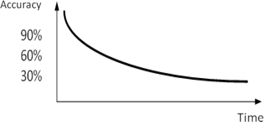
Accuracy of forecasting in time

Hot Rolled Coil is the main item of the compressor. Having analyzed the findings shown in Figure 5, we can conclude that:

Fig. 5.

Comparison between Inventory levels, Production and Orders for item Hot Rolled Coil

Large fluctuations occurs at inventory level because the uncertainty of delivery time.

Inventory level of raw material is increasing as production volume is increasing (month 3), which is abnormal. In a normal case, the inventory level of raw material should decrease when the production is increasing.

Considering the four steps proposed in Section 3 (Data selection, Preprocessing, Transformation and NN selection and training), we have obtained the following processing steps:

Data selection. This step extracts only the records of Item SQ-0231049 from the table. The inventory level of 6 months is described in Figure 6.

Data pre-processing. This step deals with data cleaning or enrichment. The records don't contain any missing values but we need to enrich the data due to the limited records from the company. Using an interpolation function (green line) we obtain the chart shown in Figure 7. Dividing each month into 4 weeks and rounding up the last two decimals, we obtain the data as listed in Table 1.

Now we have 17 samples corresponding to 17 weeks (Figure 8). The goal is to predict the demand at the 9th week and the 13th week. P1 corresponds to actual value 2632 (9th week) and P2 with the value of 2086 (13th week). The values to be forecasted are at week 9 when the inventory level is increasing, and at week 13 when the inventory level is decreasing.

Data transformation. This step converts data into a form suitable for the inputs into NN. Our data contains no categorical data (true/false) and the values are numerical, therefore no transformations are required.

NN selection and training:

We have followed two cases 4.1) and 4.2) corresponding to week 9 and week 13. We choose these two weeks because the trend is increasing in the first case (4.1) and is decreasing in the second case (4.2).

Fig. 6.

Inventory level for Item Hot Rolled Coil

Fig. 7.

Interpolation function

Fig. 8.

Inventory level records chart

Table 1.

Samples obtained after sampling

Week	1	2	3	4	5	6	7	8	9	10	11	12	13	14	15	16	17
INV LV	2118	1939	1842	1804	1796	1921	2229	2504	2632	2551	2386	2200	2086	2036	1992	1962	1952

4.1. For the first point to be predicted (2632 –actual value) we use a FFNN and a NARX network to forecast for the 9th week. The data used for input to train, validate and test the parameters is depicted in Table 2.

Table 2.

Training sample for P1

	Training set					TEST
Input	2118	1939	1842	1804	1796	1921
	1939	1842	1804	1796	1921	2229
	1842	1804	1796	1921	2229	2504
Output
	1804	1796	1921	2229	2504	2632

Table 3.

Training sample for P2

		Training set
2118	1939	1842	1804	1796	1921	2229	2504	2632	2551
1939	1842	1804	1796	1921	2229	2504	2632	2551	2386
1842	1804	1796	1921	2229	2504	2632	2551	2386	2200

1804	1796	1921	2229	2504	2632	2551	2386	2200	2086

4.2. For the second point (2086-actual value) FFNN and NARX network are trained using Table 3. Therefore we have three inputs and one output.

All the networks are using the default Levenberg-Marquardt algorithm for training. The application randomly divides input vectors and target vectors into three sets as follows:

60% are used for training.

20% are used to validate that the network is generalizing and to stop training before overfitting.

The last 20% are used as a completely independent test of network generalization.

5. Results

After training the network the performance can be evaluated using performance function (Figures 9 and 10). Even though the samples fed at the inputs during training process are few, both NNs are able to learn efficiently the pattern of the data. However, NARX network corresponding to point P1 (NARX P1) depicts a better performance in comparison with FFNN P1.

Fig. 9.

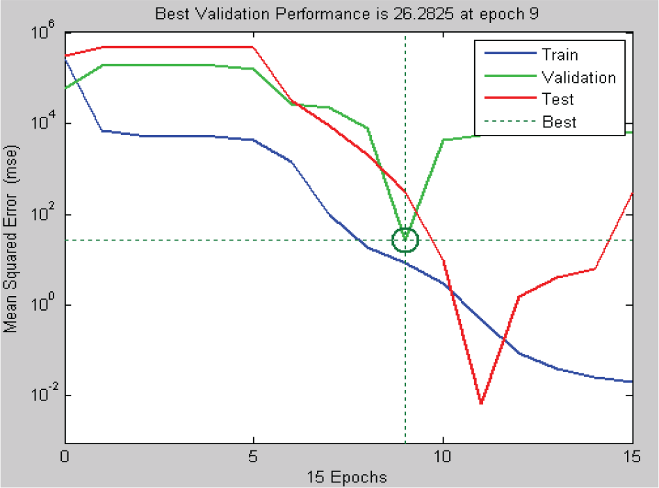
Performance analyses for FFNN P1

Fig. 10.

Performance analyses for NARX P1

Table 4.

Forecasting for P1 (2632)

	FFNNp1	NARXp1	MA(3)	ARIMA(1,0,1)
Forecast	2457	2484	2218	2451.42
ERROR	175	148	414	180.58

For a better validation of the NN models, we have also predicted the inventory levels for weeks 9 and 13, with Moving Average (MA) and ARIMA. The results are displayed in Table 4.

The error represents the difference between the predicted value in week 9 and the actual value for P1 which is 2632 (Figure 11). Results for P2 (2086) are displayed in Table 5 and Figure 12.

Fig. 11.

Graphical representation of Error for P1

Fig. 12.

Graphical representation of Error for P2

5. Discussion

In this study we have investigated the architectures of NN used to forecast demands in inventory management, and analyzed inventory level of PRD Company with the purpose of selecting an appropriate NN model to increase the forecasting accuracy. Two types of NN, FFNN and NARX, have been trained. A comparison with the traditional methods (MA and ARIMA) has been made.

In the first case (4.1) best result is obtained using a NARX NN, the difference between actual value and predicted value for week 9 is 148. For the second case (4.2) best result is obtained also by NARX NN model, the difference between actual and predicted values is only 7.

6. Conclusion

In conclusion, in a time series forecasting, best result is obtained using a NARX NN. In PRD case a NN approach can be used for each item in order to increase forecasting accuracy for the next week. Furthermore the inventory management can be improved for a better efficiency.

The ability of the NN to learn is proportional to the number of the training samples. In PRD Company case, the inventory data available is on five months, which makes NN training very difficult. Therefore we have used a fitting function which was sampled at each week in order to obtain more values. If the number of samples is increased, the learning performance can be further improved.

Future research includes:

Table 5.

Forecasting for point P 2 (2086)

	FFNNp2	NARXp2	MA(3)	ARIMA(1,0,1)
Forecast	1975	2079	2379	2097.46
ERROR	111	7	−293	−11.46

Collect more inventory data.

Validate the NN models to forecast with PRD manager's comments.

Refine the proposed model for better performance.

Footnotes

6. Acknowledgment

We would like to express our sincere gratitude and appreciation to Mr Phua, the main manager responsible for inventory at PRD Company, for his time, unmeasured patience and advices throughout this entire process.

References

Aburto

Weber

(2007) Improving supply chain management based on hybrid demand forecasts Applied Soft Computing, 7(1), pp. 136–144

Amin-Naseri

M.R.

Tabar

B Rostami

(2008) Neural Networks Approach to Lumpy demand forecasting for Proceeding of International Conference on Computer and Communication Engineering, pp.1378–1382, ISBN: 978-1-4244-1691-2 Kuala Lumpur, May 2008

Bacha

Meyer

(1992) Neural Network architecture for Load Forecasting, Proceedings of International Joint Conference on Neural Networks, pp.442–447, ISBN: 0-7803-0559-0 Baltimore, Jun 1992, IEEE Publisher, MD, USA

Back

A.D.

Wan

(1995) A unifying view of some training algorithms for MLP with FIR filter synapses, IEEE Press, pages 146–154.

Bengio

Frasconi

Simard

(1993) The problem of learning long-term dependencies in recurrent networks. Proceedings of IEEE International Conference on Neural Network, pp. 1183–1188ISBN: 0-7803-0999-5, San Francisco, Mar-Apr, 1993, IEEE Publisher, CA, USA

Conner

Martin

R Douglas

(1994) Recurrent NN and robust time series prediction. IEEE transactions on NN, 5: 240–254, 1994

Davey

Hunt

S.P.

Frank

R.J.

(1999) Time series prediction and neural networks, Journal of Intelligent and Robotic Systems, 31(1–3), pp. 91–103

Gutierrez

R.S.

Solis

A.O.

Mukhopadhyay

(2008) Lumpy demand forecasting using neural networks International Journal of Production Economics, 111(2), pp. 409–420

Larson

(1992) A generalization error estimate for nonlinear systems, Proceedings of the 1992 IEEE-SP Workshop.pp.29–38, ISBN: 0-7803-0557-4, Helsingoer, Denmark Aug- Sep 1992

10.

Lin

Tsungnan

Horne

Bill G.

Tino

Peter

Lee

Giles C.

(2000) Learning long term dependencies in NARX recurrent neural networks, Recurrent neural networks design and applications, ISBN: 9780849371813, CRC Press pp. 133–146

11.

MacKay

D.J.C.

(1994) “Bayesian non-linear modeling for the prediction competition”, Ashrae Transactions 100, pp. 1053–1062

12.

Jose

M.P. Menezes

Barreto

Guilherme A.

(2006) A new look at nonlinear time series prediction with NARX recurrent neural network, Proceedings of Ninth Brazilian Symposium on Neural Networks, pp.160–165, 23–27 Oct. 2006

13.

Moody

(1994) Prediction risk and neural network architecture selection From Statistics to Neural Networks: Theory and Pattern Recognition Applications, ISBN: 978-0387581996 Springer-Verlag

14.

Siegelmann

Hava T.

Bill

G. Horne

Lee Giles

(1997) Computational capabilities of recurrent NARX neural network” IEEE Transactions on Systems, Man and Cybernetics, Part B, 27(2), pp. 208–215.

15.

Specht

D.F.

(1991) A general regression neural network IEEE trans Neural Network, 6(2), pp. 568–576

16.

Wan

(1993) Finite impulse response neural networks with applications in time series prediction Stanford University Stanford, CA, USA

17.

Weigend

A.S.

Mangeas

Srivastava

A.N.

(1995) Nonlinear gated experts for time series: Discovering regimes and avoiding overfitting, International Journal of Neural Systems 6, pp. 373–399