
Abstract
A time delay estimation based general framework for trajectory tracking control of robot manipulators is presented. The controller consists of three elements: a time-delay-estimation element that cancels continuous nonlinearities of robot dynamics, an injecting element that endows desired error dynamics, and a correcting element that suppresses residual time delay estimation error caused by discontinuous nonlinearities. Terminal sliding mode is used for the correcting element to pursue fast convergence of the time delay estimation error. Implementation of proposed control is easy because calculation of robot dynamics including friction is not required. Experimental results verify high-accuracy trajectory tracking of industrial robot manipulators.
Introduction
Conventional model based controls of robot manipulators require calculations of nonlinear robot models [1, 2]. Implementation of these controls are not easy due to computational complexity of the robot models, and impossible if precise models of the robot manipulators are unknown. To cope with this problem, intelligent control techniques (neural-network or fuzzy logic) have received considerable attention in the last two decades [3–7]. The intelligent control techniques have the capability to approximate nonlinear functions in robot dynamics; however, they introduce a number of weighting parameters or fuzzy rules that make implementation difficult.
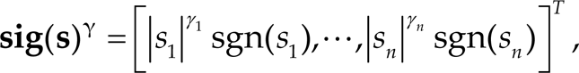
It is noteworthy that time-delay estimation (TDE) [8–11], can estimate nonlinear functions in robot dynamics simply and effectively. This approach assumes that the unknown functions do not change much for a sufficiently small time period, and estimates unknown functions by intentionally using time-delayed information of the state derivatives and control inputs. The TDE is proven to be highly efficient and effective; no off-line identification or prior knowledge of robot model is required when TDE is used; and compensation speed of TDE is faster than that of neural networks [12, 13]. The TDE technique has motivated the time delay control (TDC), which consists of two elements: the TDE element (or the auxiliary controller) and an injecting element calculated from desired error dynamics (or the error based servo controller) [9, 11].
Recently, the necessity for exploiting the third element is reported [14]. From the TDE viewpoint, the nonlinear terms in robot dynamics are classified into two categories: soft nonlinearities (including gravity, Coriolis and centrifugal torques, viscous friction, disturbance, and interaction torques) that can be estimated perfectly by the TDE; and hard nonlinearities (due to Coulomb friction, stiction) that are not compatible with the TDE [14]. When the TDE is used to estimate unknown functions, hard nonlinearities result in so-called TDE error that cause the resulting dynamics to deviate from the target dynamics; and thus lead to large tracking error. In [14], the TDE error, comes from hard nonlinearities, is suppressed by adding a third element—ideal velocity feedback term.
In this paper, a highly accurate trajectory tracking control of robot manipulators is proposed. Terminal sliding mode (TSM) [15, 16], which provides faster convergence than linear hyperplane, is used for the third element to suppress the TDE error. The proposed controller consists of three elements: a TDE element that cancels soft nonlinearities, an injection element calculated from target error dynamics, and a TSM element that suppresses the effect of hard nonlinearities. The implementation of the proposed control, due to the TDE, is easy since calculation of robot model is not required. Highly accurate position tracking control can be realized by properly choosing the fractional powers of the TSM.
The proposed control, thanks to TSM, shows a better tracking performance than Hsia's control [11] and Jin's free space tracking control [14]. Interestingly, the proposed formulation has a generalized structure: on certain conditions, the proposed control becomes Hsia's formulation [11], or Jin's free space tracking control formulation [14]. In other words, the controllers proposed in [11, 14] can be regarded as specific cases of the proposed formulation.
Benefitted from the transparent structure and simple formation of the proposed control, it is easy to provide a systematic design guideline for designing the gains. The superiority of the proposed control, especially when compared with Hsia’ and Jin's controls, is shown through simulations of a single arm and experiments of industrial manipulators, by which synergistic effects of TSM and TDE have been observed. The robustness of proposed control against parameter variations is also studied in experiments. The proposed control assures fast convergence due to the TSM, and provides model-free control due to the TDE. The proposed TDE based TSM control is practical — model-free, simple in form, highly accurate, and robust.
Compared with our previous study [17], the contents in this paper are advanced with respect to the follows: a more thorough presentation of the controller design, a more complete and rigorous stability analysis, a new design guideline for practical applications, two simulation studies including both a 1-DOF and a 2-DOF manipulator, and additional experimental studies with a 3-DOF spacial manipulator for studying the robustness of the proposed control against parameter variations.
This paper is organized as follows: In Section 2, the new control is proposed. Section 3 provides a Lyapunov based stability analysis for the closed loop dynamics. Section 4 briefly discusses properties of proposed control and presents a systematic design guideline. In Section 5, the function of TSM that compensates TDE error of hard nonlinearity is analyzed through numerical simulation. Section 6 shows the experimental results on both a SCARA-type and a PUMA-type robot manipulators. Section 7 concludes the paper.
Controller Design
Robot Dynamics
The standard form of the dynamical equation of n-DOF robot manipulator is as follows:

where
Suppose the reference input trajectory is denoted by

where
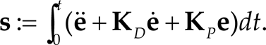
Introducing a constant, diagonal matrix,

where
The control input can be designed as

where

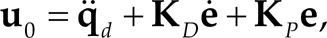
and
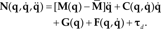
In the above control input,
The estimation of
Clearly it would be much easier to evaluate

where •t−L denotes time-delayed value of •, and L is the estimation time delay. The smallest achievable L is the sampling period in practical digital implementation. From (10), we can obtain

Thus, with the combination of (6), (7), (11), (12) the control law is expressed by

Incidentally, the past acceleration

Thanks to TDE in (11) and (12), the proposed control (13) does not use the knowledge of robot model. That is, the proposed control does not require any real-time computation of plant models, nor does it require any realtime estimation of parameters as adaptive controls do; thus, it is simple and efficient. Considering that it often takes much time and effort in practice to make a plant model or to use it for real-time purposes, this feature is truly significant from a practical viewpoint.
In this section, we first obtain the closed loop dynamics, and then based on the Tyapunov function, we prove the boundedness of the sliding surface. Two lemmas will be given before obtaining the final theorem.
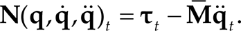
Substituting the control input (6), (7), (11) into robot dynamics (4) yields the closed loop dynamics

or

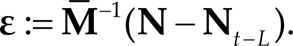
with the TDE error ε defined as
Lemma 1: Let
Lemma 2: If the control input τ (13) is applied to the robot manipulator (1), and if
Proof. Considering (7) and (15) gives

A combination of (18), (6), (7), (12), and (13) gives

From (5), the delayed nonlinear term is given by
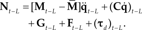
Substitute (19) into (18), and we have

where

It is clear that
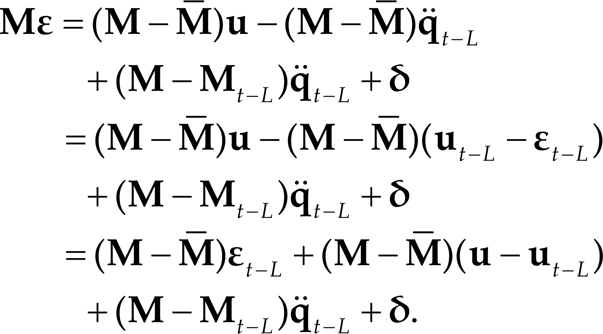
Therefore, ε is given by
where

For a sufficiently small time delay L, η1 and η2 are bounded. Note that the assumption
In the discrete-time domain (24) can be represented as

The solution of the above difference equation can be obtained as

where ε(0) is the initial value of ε(k).
Let Λ denote the maximum of

as k → ∞.
Note that ρ is a positive constant. Therefore, the TDE error ε is ultimately bounded.
Theorem 1: If the control input τ (13) is applied to the robot manipulator (1), and if the TDE error ε is bounded as a result, then the closed loop sliding surface is globally uniformly ultimately bounded.
Proof: Consider the Tyapunov function V = 1/2
Differentiating V with respect to time, and substituting (16) into it yields

where
To conclude, according to the Definition 4.6 in [21], the closed loop sliding surface is globally uniformly ultimately bounded.
Generalized Formulation
The proposed formulation (13) has a generalized structure. If

If

If

If
Due to the TDE, calculations of complex robot dynamics are unnecessary for the proposed control. The proposed control is simple and easy to implement. The nonlinear term in robot dynamics is estimated by
Function of
as a LPF
In real experiments, the encoder signal is always contaminated by noise. The noise effect is amplified when
Combining (6) and (7) leads to a compact expression of (13):

If a digital TPF with the cutoff frequency α is adopted, the control law can be modified as follows:

where

Comparing (34) with (36), if we let

then (34) and (36) are identical except the difference between
Therefore, we do not need to apply any LPF in the design of proposed control, and alternatively tune
The proposed control has five diagonal gain matrices with clear meanings. This helps simplify the design procedure, which is briefly introduced as follows.
Determine the target sliding surface (3) by selecting the desired natural frequency Select a sampling time interval L with consideration of the controller hardware. Since the TDE error in (17) becomes smaller as L becomes smaller, L is commonly chosen as small as possible. Tune β and γ should be further tuned to achieve the optimal performance.
Note that the above design procedure does not require any calculation of robot model.
Consideration regarding the state observability
In the case that some elements of the robot's state vector are not measurable, we may consider to reconstruct the state by using state observers. A model reference observer [23], [24] is useful to reconstruct states and their derivatives in a stable manner. It works quite well in the presence of plant uncertainties while preserving the control performance. Subsequently, time delay observer (TDO) [25], [26], [27] are introduced for the same purpose. These observers can be used with proposed controller when some elements of the robot's state vector are not measurable.
Simulation Studies
There are two simulation studies are performed. In Simulation One, we examine the cancellation effect of soft nonlinearities using TDE and the suppression effect of hard nonlinearities using TSM. In Simulation Two, the performance of the proposed control is evaluated in comparison with Hsia's and Jin's control.
Simulation One
Simulation Setup
For simplicity and clarity, a single arm with soft and hard nonlinearities is considered as shown in Fig. 1. The simulation parameters are as follows: The mass of the link is m = 8.163 Kg, the link length is l = 0.35 m, and the inertia is I = 1.0 Kgm2; the stiffness of the external spring as disturbance is K disturbance = 10 Nm / rad; the acceleration due to gravity is g = 9.8 Kgm / s2. Coulomb friction coefficient C c = 20 and viscous friction coefficient C v = 15. The sampling frequency of the simulation is 1 KHz.

A single arm with friction used in Simulation One.
The dynamics of a single arm is

where

The lumped soft nonlinearity and hard nonlinearity can be expressed by

Through all the comparisons, identical parameters are used for the error dynamics, as K P = 100, and K D = 20. The desired trajectory is shown in Fig. 2 and defined by

The desired trajectory used in Simulation One.

where
The simulation results are arranged in Figs. 3.— Figs. 5. Fig. 3(a) shows the soft nonlinearity

Nonlinear terms and their estimation errors. (a) Soft nonlinearity and its estimation error. (b) Hard nonlinearity and its estimation error.

The effect of TSM in the proposed control.
Two elements of the proposed control input,

Control input: target dynamics injection torque (
Simulation Setup
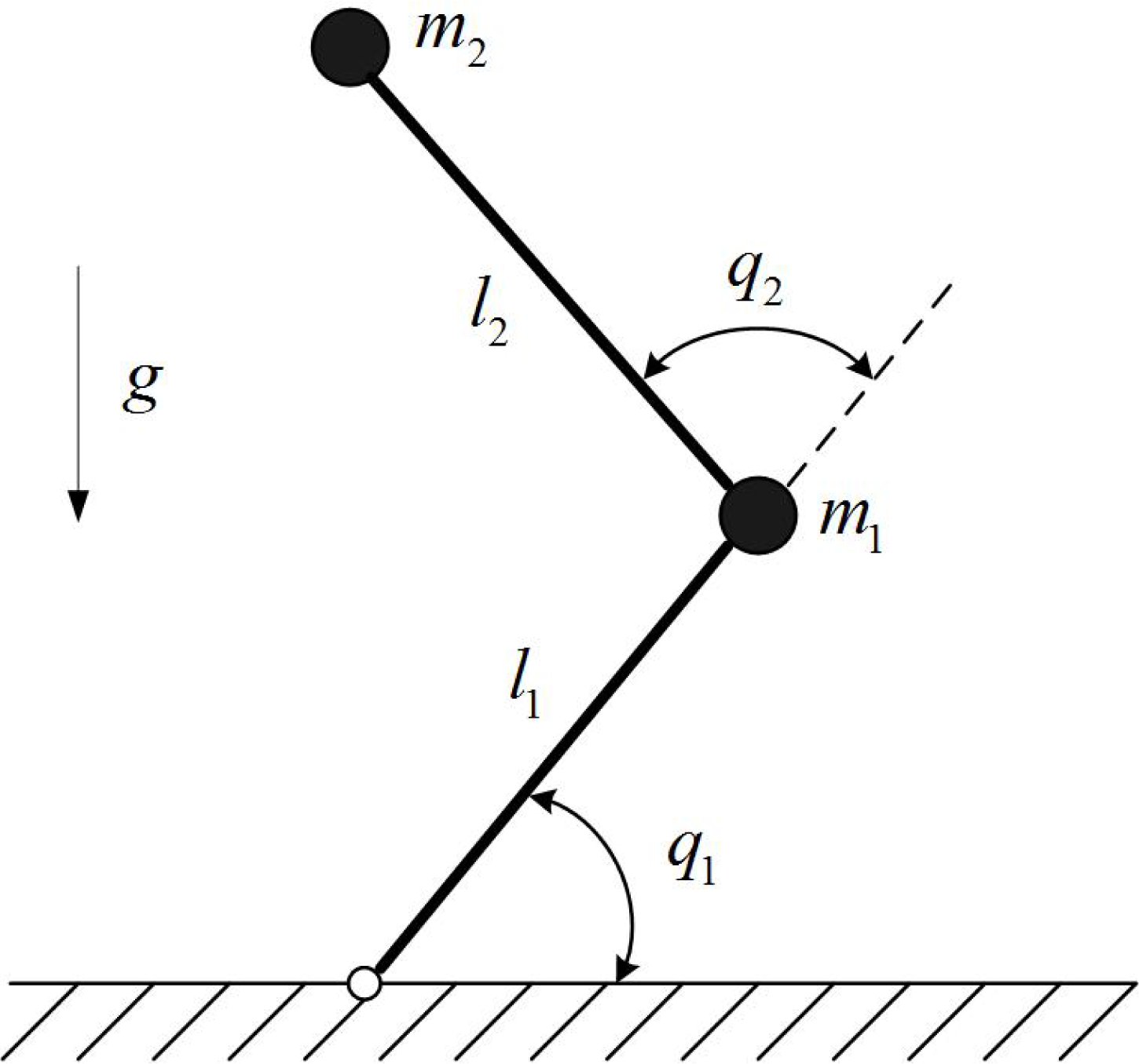
In this simulation, a 2-DOF robot manipulator is adopted as shown in Fig. 6.
The desired trajectory used in Simulation Two.
The functions in the robot dynamics (1) are given as
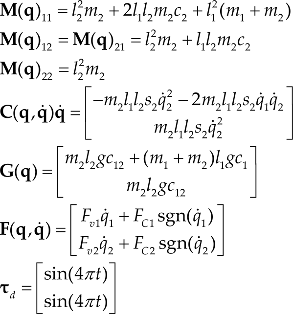
where l
i
, m
i
and F
Ci
denote the i
th
link length, mass, viscous friction coefficient, Coulomb friction coefficient, respectively; g denotes the local acceleration due to gravity, and s
i
= sin(q
i
), c
i
= cos(q
i
) and c
ij
= cos(q
i
+ q
j
);
The parameter values of the robot dynamics are
A fifth-order polynomial trajectory is used for the sixth path segments listed in Table 1., where both the initial position and the final position of each segment are listed along with the initial time and the final time. The velocity and the acceleration at the beginning and end of each segment are set to zero. The desired trajectory for both q1d and q2d are shown in Fig. 7. (a) and (b).
Initial and final position of each segment of the desired trajectory in Simulation Two.


Simulation results with a 2-DOF robot manipulator, (a) Tracking trajectory of joint 1. (b) Tracking trajectory of joint 2. (c) Tracking error of joint 1. (d) Tracking error of joint 2. (e) Control input of joint 1. (f) Control input of joint 2.
Three model-free controls are compared through simulations: Hsia's control (31), Jin's control (32), and the proposed control (13). For fair comparison, all three controllers are implemented with the same gains:

The additional parameters of Jin's control (32) are
and the additional parameters of the proposed control (13) are

The position responses, tracking errors and control inputs of both joints are respectively shown in Figs. 7. (a), (b), (c), (d), (e) and (f). The simulation results, especially the tracking error in Figs. 7. (c) and (d), demonstrate the importance of γ. Since Hsia's, Jin's and the proposed controls are equally based on the same uncertainty cancelation scheme – TDE, the performance difference is likely to be accounted for by the TSM. The peaks of the tracking error shown in Fig. 7. (c) and (d) came from the TDE error due to discontinuity of Coulomb friction [14], through which the TSM is shown effective on counteracting the tracking deviation caused by the TDE error. The proposed control shows a high-accuracy performance due to the superimposing effect of both TDE and TSM.
Experimental Studies
We have conducted two experiments to demonstrate the high-accuracy performance of the proposed control, besides which two important properties of the proposed control are studied in separate experiment. In Experiment One, the effect of γ on the tracking performance is demonstrated through a 2-DOF SCARA-type robot manipulator. In Experiment Two, the robustness of the proposed control against parameter variations is examined through a 3-DOF PUMA-type robot manipulator.
Experiment One
Experimental Setup
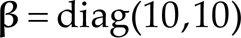
The robot used in the experiment is a 2-DOF SCARA-type robot as shown in Fig. 8. The lengths of the two links are l1 = 0.35 m and l2 = 0.29 m; and their masses are m1 = 11.17 Kg and m2 = 6.82 Kg. The distance from the joint axis to the center of mass for each link is l1 = 0.30 m and l2 = 0.18 m; the moment of inertia about the joint axis is I1 = 1.0 Kgm2 and I2= 0.224 Kgm2. At joint 1, an AC servo motor with a stall torque of 2.39Nm is used to transmit power through a harmonic drive with a gear reduction ratio of 100:1. At joint 2, a motor with a stall torque of 0.92Nm is used with a gear reduction ratio 80:1. Each joint has a resolver attached at its shaft to sense the angular displacement with the resolution of 4096 pulses/rev. The implementation of the controller was made in QNX, a real-time operating system, with a sampling frequency of 1 KHz.
A 2-DOF planar robot system.
We have experimented with the three model-free controls: Hsia's control (31), Jin's control (32), and the proposed control (13). For comparison, all three controllers are implemented with the same gains:
Circle Trajectory
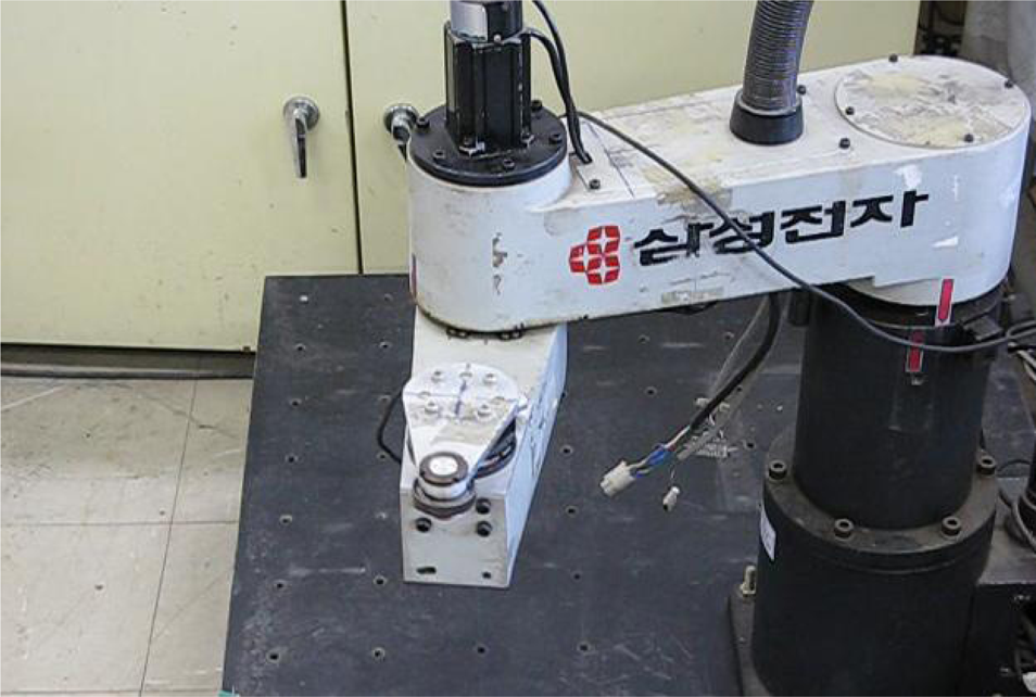
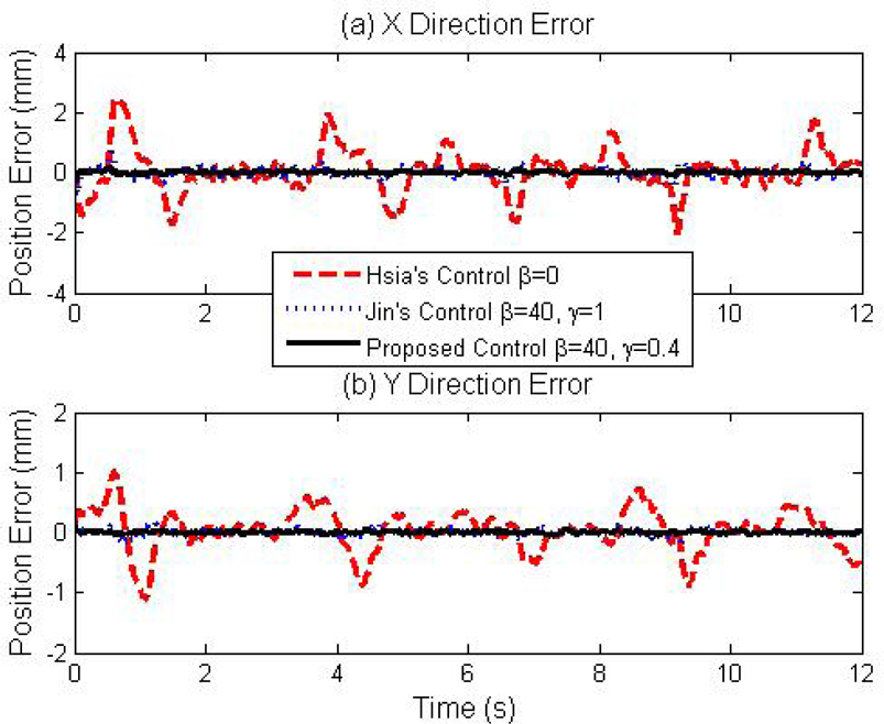
In the first group of experiments, the robot was commanded to draw a circle as shown in Fig. 9. in 4s. The experimental results are arranged in Fig. 10. and Table 2. The proposed control shows the smallest error among the three controllers. The smallest error comes as a result of the use of TSM.
Experiment One: comparison of RMS errors with circle trajectory (x10−3 m).
Experiment One: comparison of RMS errors with circle trajectory (x10−3 m).


Experiment One: the desired circle trajectory.

Experiment One: comparison of position error with circle trajectory. (a) X direction (b) Y direction.
Fig. 11 shows root mean square (RMS) error, where γ = diag(0.4,0.4) shows the smallest error. Both γ = diag(0,0) (33) and γ = diag(1,1) (32) show larger error than TSM. By properly choosing the fractional powers, a trade-off between tracking precision and robustness to unmodeled dynamics can be obtained. The proposed control can enjoy benefits of both high precision and chattering attenuation.

Experiment One: comparison of root mean square error with circle trajectory, (a) X direction (b) Y direction.
Chaotic Trajectory
The chaotic trajectory is widely applied for effective fluid mixing [28], which is a key issue in contemporary systems for micro-total analysis.
In the second group of experiments, the robot was commanded to follow a chaotic trajectory [29] whose dynamics is

where xm1, xm2 and xm3 are state variables. The parameters of the above Tu system are selected to be a = 35, b = 3 and c = 20. The initial values of the desired chaotic system are xm1 = −10, xm2 = −5, and xm3 = 5. The 3D phase portrait of the above trajectory is shown in Fig. 12. Regarding the fact that the robot under control is a 2-DOF planar robot, xm2 and xm3 were chosen as the desired states of joint1 and joint2 respectively, whose phase portrait is shown in Fig. 13.

Experiment One: 3D desired chaotic trajectory.

Experiment One: 2D desired chaotic trajectory.
The experimental results are arranged in Fig. 14 and Table 3. The proposed control shows the smallest error among the three controllers. The smallest error comes as a result of the use of TSM.
Experiment One: comparison of RMS errors with chaotic trajectory (x10−3 m).

Experiment One: comparison of position error with chaotic trajectory, (a) X direction (b) Y direction.
Fig. 15 shows root mean square (RMS) error, where γ = diag(0.4,0.4) shows the smallest error. Both γ = diag(0,0) (31) and γ = diag(1,1) (32) show larger error than TSM. By properly choosing the fractional powers, a trade-off between tracking precision and robustness to unmodeled dynamics can be obtained. The proposed control can enjoy benefits of both high precision and chattering attenuation.

Experiment One: comparison of root mean square error with chaotic trajectory, (a) X-direction (b) Y-direction.
Experimental Setup
The robot used in the experiment is a 3-DOF PUMA-type robot as shown in Fig. 16. The maximum payload of the robot is 3 Kg, and the maximum continuous torques are 0.637, 0.637, and 0.319 Nm for joints 1, 2, and 3, respectively. The gear reduction ratio and the encoder resolution of each joint are 120:1 and 8192 pulses/rev, respectively. Resolution of each robot joint is 3.66 × 10⁻⁴ deg. The parameters of robot dynamics were assumed to be unknown, and thus were not used. All of the joints are commanded by the same trajectory shown in Fig. 17. The sampling time L is selected as 0.001 s.

(Left) A 3-DOF PUMA-type robot in which the positive directions are denoted by arrows. (Right) The 3-DOF PUMA-type robot with a 2.15 kg payload.

Experiment Two: the desired trajectory.
We have experimented with total three model-free controls: Hsia's control (31), Jin's control (32), and the proposed control (13). For comparison, all three controllers are implemented with the same gains:

The additional parameters of Jin's control (32) are
and the additional parameters of the proposed control (13) are

The design of controllers followed the guideline presented in subsection 3.4 and did not require any calculation of robot model.
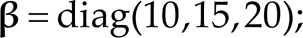
The experimental results are arranged in Fig. 18. and Table 4., and the tendency is in good agreement with simulation results. Examining the tracking errors of Jin's and proposed control shown in Figs. 18. (a), (c) and (e), the proposed control shows far better tracking performance, justifying the effect of γ on the further improvement of the tracking accuracy. The peaks of the tracking error around t = 0s, 5s, 15s came from the TDE error due to discontinuity of Coulomb friction [14]. The TSM is shown effective on counteracting the tracking deviation caused by the TDE error as shown in Figs. 18. (a), (c) and (e).
Experiment Two: comparison of RMS errors with other two model-free controllers (x10−3 deg).
Experiment Two: comparison of RMS errors with other two model-free controllers (x10−3 deg).

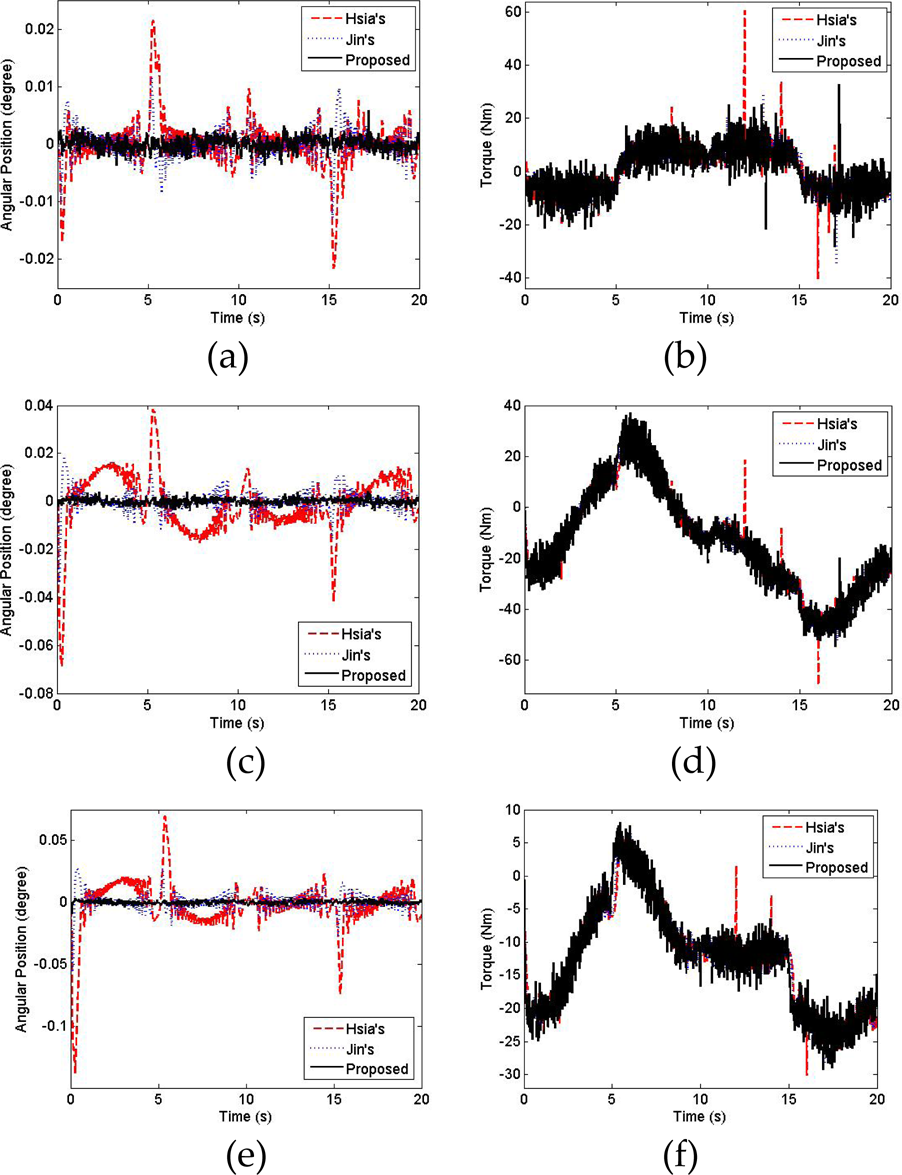
Experiment Two: experimental results with a 3-DOF robot manipulator. (a) Tracking error of joint 1. (b) Control input of joint 1. (c) Tracking error of joint 2. (d) Control input of joint 2. (e) Tracking error of joint 3. (f) Control input of joint 3.
The root-mean-squared (RMS) errors of proposed control in Table 4. reveal that the obtained performance is highly accurate regarding the resolution of robot. Figs. 18. (b), (d) and (f) show that the control inputs are a little noisy but bounded without any noticeable control chatterings. The proposed control can enjoy benefits of both high precision and chattering attenuation.
In order to show the robustness of the proposed control against parameter variations, we first tuned the proposed control for no-payload condition, and then verified the performance using the same gains with a 2.15 Kg payload (72% of maximum payload). The experimental results are shown in Fig. 19. and Table 5. The tracking performances of the proposed control with or without payload are quite similar. More precisely, the RMS errors in Table 5. show that only joint 3 has a slight performance degradation. The control input magnitude of joints 2 and 3 is increased to compensate the payload gravity as shown in Figs. 19. (d) and (f).
Experiment Two: comparison of RMS errors by proposed control without or with payload (x10−3 deg).
Experiment Two: comparison of RMS errors by proposed control without or with payload (x10−3 deg).


Experiment Two: experimental results of the proposed control without payload (black solid) and with a 2.15 kg payload (red dotted). (a) Tracking error of joint 1. (b) Control input of joint 1. (c) Tracking error of joint 2. (d) Control input of joint 2. (e) Tracking error of joint 3. (f) Control input of joint 3.
To summarize, high accuracy control can be realized through the proposed control by using both TDE and TSM.
A time delay estimation based general framework for trajectory tracking control of robot manipulators is presented. The controller consists of three elements: a time-delay-estimation element that cancels continuous nonlinearities of robot dynamics, an injecting element that endows desired error dynamics, and a correcting element that suppresses residual time delay estimation error caused by discontinuous nonlinearities. Terminal sliding mode is used for the correcting element to pursue fast convergence of the time delay estimation error. Implementation of proposed control is easy because calculation of robot dynamics including friction is not required.
Synergistic effects have been obtained with the combination of the TSM and the TDE through both simulations and experiments. The proposed control assures fast convergence due to the TSM, and provides mode-free control due to the TDE, which facilitates an effective and efficient control. It was verified through both simulations and experiments that the proposed control is easily implementable and highly accurate. The proposed TDE based TSM control is practical—model-free, simple in form, highly accurate, and robust.