Sage Journals: Discover world-class research

Abstract

Differential kinematic is one of the most important solution methods in robot kinematics. The main advantage of the differential kinematic method is that it can be easily implemented any kind of mechanisms. Also, an accurate and efficient kinematic based trajectory tracking application can be easily implemented by using this method. In differential kinematic method, we use Jacobian as a mapping operator in the velocity space. Inversion of Jacobian matrix transforms the desired trajectory velocities, which are the linear and angular velocities of the end effector, into the joint velocities. The joint velocities are required to be integrated to obtain the pose of the robot manipulator. This integration can be evaluated by using numerical integration methods, since the inverse kinematic equations are highly complex and nonlinear. Therefore, the performance of the trajectory tracking application of the robot manipulator is directly affected by the chosen numerical integration method. This paper compares the performances of numerical integration methods in the trajectory tracking application of redundant robot manipulators. Several widely used numerical integration methods are implemented into the trajectory tracking application of the 7-DOF redundant robot manipulator named PA-10 and simulation results are given.

Keywords

Differential Kinematics Jacobian Numerical Integration Redundant Robot Manipulators Trajectory Tracking

1. Introduction

The configurations of redundant robot manipulators offer the potential to overcome many difficulties by increased manipulation ability and versatility [1, 2]. A desired trajectory can be tracked in many different configurations of redundant robot manipulators by using the extra manipulation ability. This feature can be easily implemented into the many robotic applications such as obstacle avoidance, singularity avoidance, complex manipulation etc. [3, 4 and 5]. Redundant robots are also frequently used in complex industrial applications, service robots and humanoids [6]. However the redundant robot manipulators have many advantageous, they require quite complex control structures and suffer from singularity problem.

A fundamental research task of redundant robot manipulation is to find out the appropriate way to control the system of redundant robot manipulator in the work space at any stage of the trajectory tracking. This control can be achieved by using dynamic or kinematic model based control. However, dynamic model based control gives us more realistic results than kinematic based control, it requires highly complex control structures. Therefore, it is generally used to control the few degrees of freedom (DOF) robot manipulators in the laboratory researches [7, 8]. Kinematic model based control can also be used to solve the problem of redundant robot manipulation. In the kinematic problem, the equation of motion is obtained without using the forces and torques which cause the motion and more elegant control structures can be obtained due to the nature of the kinematic problem. However kinematic model based control is not as realistic as dynamic model based control, it has a quite simple control structure and it can be easily implemented to the robotic problems which do not require force and torque controls. Therefore, kinematic model based control is widely used in many robotics applications such as industrial robotics [9, 10].

Differential kinematic is one of the most important solution methods in robot kinematics [11,12]. The main advantage of the differential kinematic is that it can be easily implemented any kind of mechanism. Also, an accurate and efficient kinematic based trajectory tracking applications can be easily implemented by using this method [13]. Jacobian is used as a velocity mapping operator which transforms the joint velocities into the Cartesian linear and angular velocities of the end effector. A highly complex and nonlinear inverse kinematic problem of redundant robot manipulators can be solved numerically by just inversing the Jacobian matrix operator. However, differential kinematic based solutions can be easily implemented any kind of mechanisms, it has some disadvantages. The first one is that differential kinematic based solutions are locally linearized approximation of the inverse kinematic problem [14]. Thus, we can only obtain the approximate solutions of the inverse kinematic problem by using this method. Although the solution results of this method are not real, the approximation results are generally quite sufficient for small joint velocities. The second disadvantage of this method is that it has a heavy computational load and big computational time because of numerical iterative approach [7]. Requirement of the inversion of Jacobian matrix operator directly affects the computational efficiency in the inverse kinematics. Moreover, this requirement also causes the singularity problem. Singularity is one of the most important problems in robot kinematics [15]. At or around the singular configurations of robot manipulator, Jacobian transformation generates high joint velocities which results in instability and large errors in the task space. Several studies have been published on the problem of kinematic singularity in the literature. In general, there are four main techniques to cope with the kinematic singularity problems. These are avoiding singular configuration method, robust inverse method, a normal form approach method and extended Jacobian method [16 –19]. However given techniques have some disadvantages which include computational load and errors. And the last disadvantage of the differential kinematics method is that, it requires numerical integration which suffers from numerical errors, to obtain the joint positions from the joint velocities [20]. The numerical integration of joint velocities to compute joint positions causes a numerical drift which in turn corresponds to a task space error [21, 22]. An effective inversion of differential kinematics mappings can be realized by adopting the so-called closed-loop inverse kinematics algorithms which are based on the use of a feedback correction term on the task space error [23]. However the drift-phenomena can be overcome by using the closed-loop inverse kinematic algorithm, the performance of the algorithm is still extremely affected by the chosen numerical integration method.

In numerical integration, we calculate the analytical integral approximately by using numerical techniques. This computation can also be called as quadrature [24]. There are a wide range of quadrature methods available in the literature [25 –28]. Accuracy and performance are main requirements in the quadrature algorithms. In general, better accuracy can be obtained by increasing the computational complexity and computational load. Therefore, this case, in general, results as a trade-off between the accuracy and computational performance in the numerical integration algorithms.

In this paper, a performance analysis of the numerical integration methods in the trajectory tracking application of the redundant robot manipulators is presented in details. Three single-step numerical integration methods which are Euler integration, Runge-Kutta 2 and Runge-Kutta 4 and also three multi-step numerical integration methods which are Predictor & Corrector, Adams-Bashforth and Adams-Moulton methods are implemented into the differential kinematic based solution of the trajectory tracking application of the redundant robot manipulator. These methods are compared with respect to computational efficiency and accuracy. Simulation results of the trajectory tracking are given in section V. This paper is also included the differential robot kinematics in section II, numerical integration methods in section III, trajectory tracking algorithms in section IV. Conclusions and future works are drawn in the final section.

2. Differential Robot Kinematics

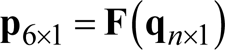
It is so hard, even impossible to find the analytical solutions of the inverse kinematic problem of the redundant robot manipulators except the limited special structures or very simple mechanisms. Therefore, differential kinematic based solution of the inverse kinematic problem of the redundant robot manipulators is widely used [29]. Differential kinematic based solution can be formulated as follows,

Let's p define the pose, which includes the position and orientation, of the end effector. It can be formulated in terms of the joint angles as follows,

p_{6 \times 1} = F (q_{n \times 1})

(1)

where q_n×1 = [q₁ q₂ ⃛ q_n] indicates the joint angles and n is the number of the joints. If we differentiate it then, we get,

\dot{p} = \dot{F} (q_{n \times 1}) = \frac{\partial F}{\partial q} \dot{q} = V_{t}

(2)

where $\frac{\partial F}{\partial q} = [\begin{matrix} \frac{\partial F_{1}}{\partial q_{1}} & \frac{\partial F_{1}}{\partial q_{2}} & \dots & \frac{\partial F_{1}}{\partial q_{n}} \\ \frac{\partial F_{2}}{\partial q_{1}} & \frac{\partial F_{2}}{\partial q_{2}} & \dots & \frac{\partial F_{2}}{\partial q_{n}} \\ ⋮ & ⋮ & ⋮ & ⋮ \\ \frac{\partial F_{6}}{\partial q_{1}} & \frac{\partial F_{6}}{\partial q_{2}} & \dots & \frac{\partial F_{6}}{\partial q_{2}} \end{matrix}]$ is the Jacobian matrix and $\dot{q} = [\begin{matrix} {\dot{q}}_{1} & {\dot{q}}_{2} & \dots & {\dot{q}}_{n} \end{matrix}]$ is the joint velocities. V_t indicates the end effector's velocities. As it can be directly seen from the equation (2), Jacobian is a mapping operator which transforms the joint velocities into the Cartesian velocities. Joint velocities can be obtained by using the inversion of the Jacobian matrix operator as the following,

\dot{q} = J^{g} (q) V_{t}

(3)

where J^g (q) indicates generalized inverse of the Jacobian matrix. In the introduction part, we mentioned about that differential kinematic based solution is a locally linearized approximation of the inverse kinematics solution [30]. It can be directly seen by using the Taylor expansion of the forward kinematics equation. It can be formulated as follows,

F (q) = F (q_{0}) + {\frac{\partial F (q)}{\partial q} Δ q |}_{q = q_{0}} + \frac{1}{2!} {\frac{\partial^{2} F (q)}{\partial q^{2}} {(Δ q)}^{2} |}_{q = q_{0}} + \dots

(4)

If we assume that Δq is relatively small then, we can omit the high order terms of the Taylor expansion. Then, we get the approximate solution as the following,

F (q) = F (q_{0}) + {\frac{\partial F (q)}{\partial q} Δ q |}_{q = q_{0}} = F (q_{0}) + {J (q) Δ q |}_{q = q_{0}}

(5)

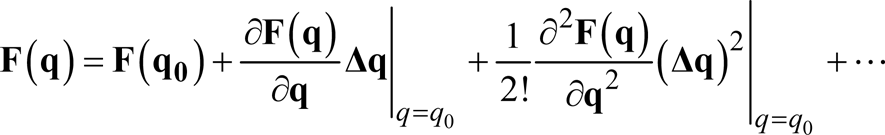
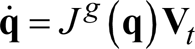
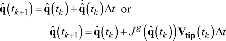
As it can be directly seen from the equation (5) differential kinematic based solution is locally linearized approximation. This equation is admissible if the Δq is small enough and the higher order terms of the Taylor series can be neglected. Also the equation (5) equals to a simply first order Euler integration.

The joint velocities should be integrated to obtain the joint positions by using the following equation,

q = \int_{t_{1}}^{t_{2}} \dot{q} d t = \int_{t_{1}}^{t_{2}} J^{g} (q) V_{t} d t

(6)

As it can be seen from the equation (6), the integrand is highly complex and nonlinear. Analytical solution of this integration, in general, is so hard, even impossible. Therefore, numerical integration methods should be used to solve this problem. The numerical integration solution techniques of the equation (6) will be discussed in the next section.

Note that, we derived the Jacobian operator analytically in this section. However, different methods can be used to find the Jacobian operator. Several methods to obtain the Jacobian operator can be found in [31 –33]

3. Numerical Integration of The Joint Velocities

Iterative solution methods are generally used to solve the inverse kinematic problem of the redundant robot manipulators because of highly complex and nonlinear inverse kinematic equations. The joint angles are obtained by numerically integrating the joint velocities. Therefore, the chosen numerical integration method extremely affects the computational efficiency and accuracy of the differential kinematic based trajectory tracking algorithm.

Here, several numerical integration methods are introduced. These integration methods can be divided into two main different approaches which are single-step and multi-step numerical integration methods. The formulations of these integration methods are as the following, [25 –27]

A. Single-Step Numerical Integration Methods

• Explicit Euler Integration Method:

Explicit Euler integration is the simplest numerical integration method. It is simply the first order Taylor expansion and formulated as follows

q (t_{k + 1}) = q (t_{k}) + \dot{q} (t_{k}) Δ t

(7)

where \dot{q} (t_{k}) = J^{g} (q (t_{k})) V_{t} (t_{k})

(8)

The strength of this method is that it can be easily implemented and also it has a very computationally light algorithm. However, the accuracy of this method is quite poor. It requires small sampling rates to obtain stable and accurate results.

Runge-Kutta 2 Method:

Runge-Kutta methods are one of the most widely used numerical integration methods. The formulation of the second order Runge-Kutta numerical integration method is as follows,

q (t_{k + 1}) = q (t_{k}) + ({\dot{q}}_{1} (t_{k}) + {\dot{q}}_{2} (t_{k})) \frac{Δ t}{2}

(9)

where ${\dot{q}}_{1} (t_{k}) = J^{g} (q (t_{k})) V_{t} (t_{k})$ and

{\dot{q}}_{2} (t_{k}) = J^{g} (q_{1} (t_{k})) V_{t} (t_{k + 1})

(10)

in which q_{1} (t_{k}) = q (t_{k}) + J^{g} (q (t_{k})) V_{t} (t_{k}) Δ t

(11)

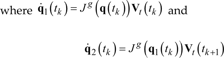
This method requires two calculations of the generalized inverse Jacobian for each step, so that the computational load of this method is higher than Explicit Euler integration. However it requires extra computation, it gives more accurate and stable results than Explicit Euler integration.

Runge-Kutta 4 Method:

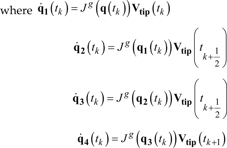
The formulation of the fourth order Runge-Kutta numerical integration method is as follows,

q (t_{k + 1}) = q (t_{k}) + \frac{1}{6} ({\dot{q}}_{1} (t_{k}) + 2 {\dot{q}}_{2} (t_{k}) + 2 {\dot{q}}_{3} (t_{k}) + {\dot{q}}_{4} (t_{k}))

(12)

where ${\dot{q}}_{1} (t_{k}) = J^{g} (q (t_{k})) V_{t i p} (t_{k})$

\begin{array}{l} {\dot{q}}_{2} (t_{k}) = J^{g} (q_{1} (t_{k})) V_{t i p} (t_{k + \frac{1}{2}}) \\ {\dot{q}}_{3} (t_{k}) = J^{g} (q_{2} (t_{k})) V_{t i p} (t_{k + \frac{1}{2}}) \\ {\dot{q}}_{4} (t_{k}) = J^{g} (q_{3} (t_{k})) V_{t i p} (t_{k + 1}) \end{array}

(13)

in which $q_{1} (t_{k}) = q (t_{k}) + \frac{Δ t}{2} (J^{g} (q (t_{k})) V_{t i p} (t_{k}))$

\begin{array}{l} q_{2} (t_{k}) = q (t_{k}) + \frac{Δ t}{2} (J^{g} (q_{1} (t_{k})) V_{t i p} (t_{k + \frac{1}{2}})) \\ q_{3} (t_{k}) = q (t_{k}) + Δ t (J^{g} (q_{2} (t_{k})) V_{t i p} (t_{k + \frac{1}{2}})) \end{array}

(14)

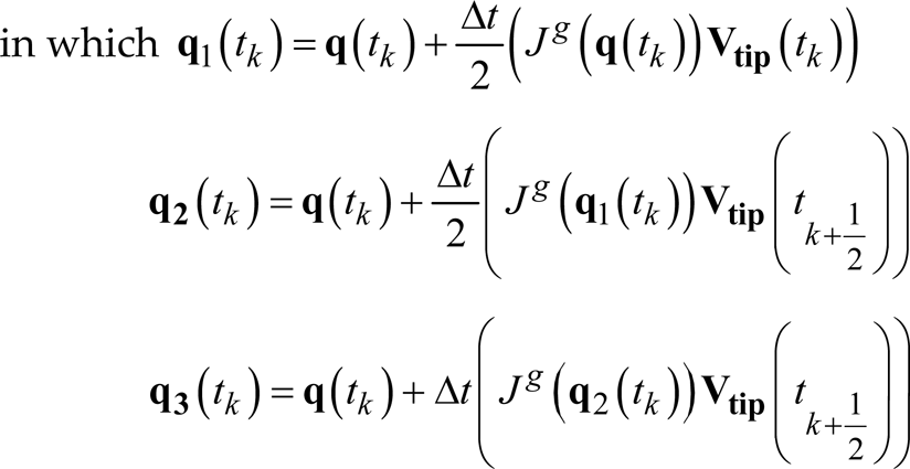
This method requires four calculations of the generalized inverse Jacobian for each step, so that the computational load of this method is higher than Runge-Kutta 2. This extra computation improves the numerical integration results and the solutions, which are more accurate and stable than Runge-Kutta 2 based solutions, can be derived by using this method. As the order of the Runge-Kutta numerical integration method increases, more accurate and stable results are obtained by using more computationally complex algorithms.

B. Multi-Step Numerical Integration Methods

Euler Trapezoidal Predictor & Corrector Method:

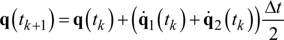
Euler Trapezoidal Predictor & Corrector method is an algorithm that proceeds in two steps. First, the prediction step calculates a rough approximation of the desired quantity. In this step simple Explicit Euler integration is used. Second, the corrector step refines the initial approximation using another means. In this step trapezoidal integration is evaluated by using the predicted and current joint velocities. The formulation of this method is as follows,

q (t_{k + 1}) = q (t_{k}) + \frac{Δ t}{2} (\dot{q} (t_{k}) + \dot{\hat{q}} (t_{k + 1}))

(15)

where $\dot{\hat{q}} (t_{k})$ is the predicted joint velocity vector in which

\begin{array}{l} \hat{q} (t_{k + 1}) & = & \hat{q} (t_{k}) + \dot{\hat{q}} (t_{k}) Δ t or \\ \hat{q} (t_{k + 1}) = \hat{q} (t_{k}) + J^{g} (\hat{q} (t_{k})) V_{t i p} (t_{k}) Δ t \end{array}

(16)

Euler Trapezoidal Predictor & Corrector method also requires two computation of the generalized inverse of Jacobian operator so that the computational load increases. It gives more accurate and stable results than Explicit Euler Integration.

Adams-Bashforth Method (Fourth Order):

Adams-Bashforth is a widely used multi-step explicit numerical integration method. It can be formulated as follows,

If t_{k} = t_{1} then q (t_{k + 1}) = q (t_{k}) + \dot{q} (t_{k}) Δ t,

(17)

If t_{k} = t_{2} then q (t_{k + 1}) = q (t_{k}) + \frac{Δ t}{2} (3 \dot{q} (t_{k}) - \dot{q} (t_{k - 1}))

(18)

If $t_{k} = t_{3}$ , then

q (t_{k + 1}) = q (t_{k}) + \frac{Δ t}{12} (23 \dot{q} (t_{k}) - 16 \dot{q} (t_{k - 1}) + 5 \dot{q} (t_{k - 2}))

(19)

If $t_{k} \geq t_{4}$ , then

q (t_{k + 1}) = q (t_{k}) + \frac{Δ t}{24} (55 \dot{q} (t_{k}) - 59 \dot{q} (t_{k - 1}) + 37 \dot{q} (t_{k - 2}) - 9 \dot{q} (t_{k - 3}))

(20)

where $\dot{q} (t_{k}) = J^{g} (q (t_{k})) V_{t i p} (t_{k})$

Several different order of this method can be used to obtain the numerical integration. Here, we used the fourth order Adams-Bashforth numerical integration algorithm which is the most widely used one. This method requires three step backward values of joint velocities and one computation of generalized inverse of Jacobian operator for each step so that it is a computationally light numerical integration method. As the order of the method increases, more accurate and stable results are obtained.

• Adams-Moulton Method (Fourth Order):

Adams-Moulten is also a widely used multi-step implicit numerical integration method. Here, Adams-Bashforth algorithm is used in the numerical integration of the predicted joint velocities and Adams-Moulton algorithm is used in the numerical integration of the corrected joint velocities. It can be formulated as follows,

If t_{k} = t_{1} then q (t_{k + 1}) = q (t_{k}) + \frac{Δ t}{2} (\dot{\hat{q}} (t_{k + 1}) + \dot{q} (t_{k})),

(21)

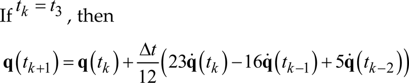
If t_t = t₂, then

q (t_{k + 1}) = q (t_{k}) + \frac{Δ t}{12} (5 \dot{\hat{q}} (t_{k + 1}) + 8 \dot{q} (t_{k}) - \dot{q} (t_{k - 1}))

(22)

If t_t ≥ t₃, then

q (t_{k + 1}) = q (t_{k}) + \frac{Δ t}{24} (9 \dot{\hat{q}} (t_{k + 1}) + 19 \dot{q} (t_{k}) - 5 \dot{q} (t_{k - 1}) + \dot{q} (t_{k - 2}))

(23)

where $\dot{\hat{q}} (t_{k})$ is the predicted joint velocities in which

\hat{q} (t_{k + 1}) = \hat{q} (t_{k}) + \frac{Δ t}{24} (55 \dot{\hat{q}} (t_{k}) - 59 \dot{\hat{q}} (t_{k - 1}) + 37 \dot{\hat{q}} (t_{k - 2}) - 9 \dot{\hat{q}} (t_{k - 3}))

(24)

Here, we used the fourth order Adams-Moulten numerical integration algorithm which is the most widely used one. This method requires two step backward values of joint velocities and one step forward predicted joint velocities. It also requires two computations of generalized inverse of Jacobian operator for each step so that computationally load increases. This extra computation improves the numerical integration results and the solutions which are more accurate than Adams-Bashforth based solutions, can be derived by using this method. As the order of the method increases, more accurate and stable results are obtained.

4. Trajectory Tracking Application

The trajectory tracking application of the redundant robot manipulator is implemented by using the following two simulink block diagrams which are shown in figures 1 and 2. The first one shows us the trajectory tracking application by using the explicit numerical integration methods which are Explicit Euler Integration, Runge-Kutta 2, Runge-Kutta 4, and Adams-Bashforth methods. In this application, a desired trajectory is generated for the end effector of the robot arm in the Desired Trajectory block and it is transferred to the Jacobian block. In the Jacobian block, the joint velocities are obtained by using the velocity mapping. Inputs of the Jacobian block are tip point velocities, error and positions of the robot manipulators. The tip point velocity input, which are linear and angular velocities of the robot manipulator, is the desired trajectory. The error input is used to obtain the closed loop inverse kinematic solution, which can be shown in figure 1. Closed loop inverse kinematics is used to cope with the drift phenomena [12]. And the position input is used to obtain the Jacobian iteratively in each step of the simulation. Joint velocities are generated in the Jacobian block and then, they are transferred to the Numerical Integration block. In the Numerical Integration block, explicit numerical integration methods, which are Explicit Euler Integration, Runge-Kutta 2, Runge-Kutta 4, and Adams-Bashforth, are used to obtain the joint angles. The obtained joint angles are transferred to the Forward Kinematics block. In the Forward Kinematics block, we obtain the pose of the robot manipulator's and the positions of the each robot manipulator's joints. The positions of each robot manipulator's joints are required to obtain the Jacobian operator iteratively. Therefore, these joint positions are transferred to the Jacobian block. Also, the pose of the robot manipulator is obtained in the Forward Kinematics block. The pose of the robot arm is required to obtain the Jacobian operator iteratively and also the closed-loop kinematic structure. Therefore, the pose of the robot arm is also transferred to the Jacobian block. The error of the trajectory tracking is calculated by using the following formulas, Let's assume that p_d and p are, respectively, the desired and actual positions of the robot arm and also R_d and R are, respectively, the desired and actual orientation of the robot arm in the direction cosine form. The position and orientation errors can be calculated by using the following equations,

p_{e} = p_{d} - p

(25)

Figure 1.

Simulink Block Diagram of Trajectory Tracking Simulation Application

Figure 2.

Simulink Block Diagram of Predictor Based Trajectory Tracking Simulation Application

o_{e} = \frac{1}{2} (R (1) \times R_{d} (1) + R (2) \times R_{d} (2) + R (3) \times R_{d} (3))

(26)

where R(1),R(2),R(3),R_d(1),R_d(2),R_d(3)define the first, second and third column vectors of the orientation matrices respectively.

The second simulink block diagram shows us the trajectory tracking application by using the implicit numerical integration methods which are Euler Trapezoidal Predictor & Corrector and Adams-Moulton integration methods. As it can be seen from the figure 2, there are three main blocks in this simulink block diagram. The first one is Desired Trajectory block which is similar as the previous one. The second one is Trajectory Tracking Algorithm block. This block includes Jacobian, Numerical Integration and Forward Kinematics blocks and they work similarly as the previous one. And the last one is Trajectory Tracking Algorithm (Predictor) block. This block also includes Jacobian, Numerical Integration and Forward Kinematics blocks and they also work similarly as the previous one. The predicted joint velocities, which are required for the implicit integration methods, are obtained by using the explicit integration methods such as Explicit Euler Integration and Adams Bashforth in the Predictor block. Then the predicted joint velocities are implemented to the Trajectory Tracking Algorithm block and implicit integrations are calculated.

5. Simulation Results

A redundant anthropomorphic robot arm structure that is shown in figure 3 is used for the simulation studies. Anthropomorphic robot arm structure is widely used in many robotics applications such as industrial applications (i.e. welding assembly etc.) and non-industrial applications (i.e. rehabilitation, human motion assistance, etc.) [34, 35]. The robot structure which is shown in figure 3 is obtained by using the Mitsubishi PA-10 anthropomorphic robot arm. Mitsubishi PA-10 robot arm features an articulated arm with 7-DOF for high flexibility. It spreads a wide range area in many robot applications. Simulation studies of the trajectory tracking application are performed by using Matlab and the animation applications are performed by using virtual reality toolbox (VRML) of Matlab which can be seen in figure 3.

Figure 3.

PA-10 Robot arm animation in virtual reality toolbox (VRML)

A circular trajectory tracking application is implemented by using the proposed kinematic control structure. Figures 4, 5 and 6 show the trajectory tracking application results. The desired and actual paths are shown in the figure 4. Joints positions and velocities are given in the figures 5 and 6.

Figure 4.

Path tracking on the coordinates x and y

Figure 5.

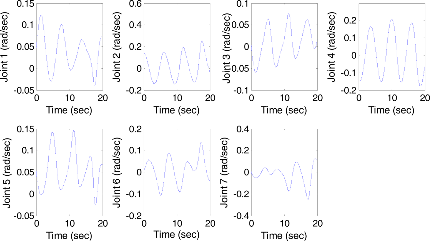
Joint velocities of robot arm during the circular trajectory tracking application

Figure 6.

Joint positions of robot arm during the circular trajectory tracking application

As it can be seen from the figures 4, 5 and 6 a satisfactory trajectory tracking application is implemented for the desired circular path. The circular path is tracked precisely as shown in figure 4. Also, both of the joint positions and velocities are smooth during the trajectory tracking application as shown in figures 5 and 6. In this trajectory tracking application, Runge-Kutta 4 is used for the real time numerical integration with Δt = 100 ms sampling rate.

There are two main requirements, which are accuracy and computational efficiency, in the real time numerical integration applications. The computational efficiency performances of the proposed numerical integration methods in the trajectory tracking application can be seen in the figures 7 and 8.

Figure 7.

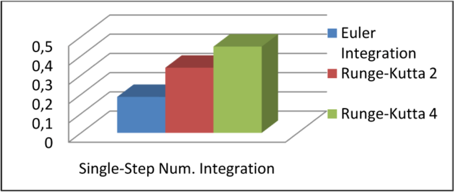
Simulation times of the single-step numerical integration based solutions (sec)

Figure 8.

Simulation times of the multi-step numerical integration based solutions (sec)

As it can be directly seen from the figures 7 and 8 the most computationally efficient method is Explicit Euler Integration and the least computationally efficient method is Runge-Kutta 4. The computational efficiency results of the numerical integration methods are quite similar. However, these small performance differences of the numerical integration methods may drastically affect the performance of the real time application. The computation time is evaluated by using Matlab's tic-toc commands. Running environment is as follows,

Accuracy is the other important requirement in the numerical integration applications. The accuracies of the proposed numerical integration methods are analyzed in

C. Single-Step Numerical Integration Methods

• Explicit Euler Integration

the trajectory tracking application and the simulation results are given in the figures 9, 10, 11, 12, 13 and 14.

Figure 9.

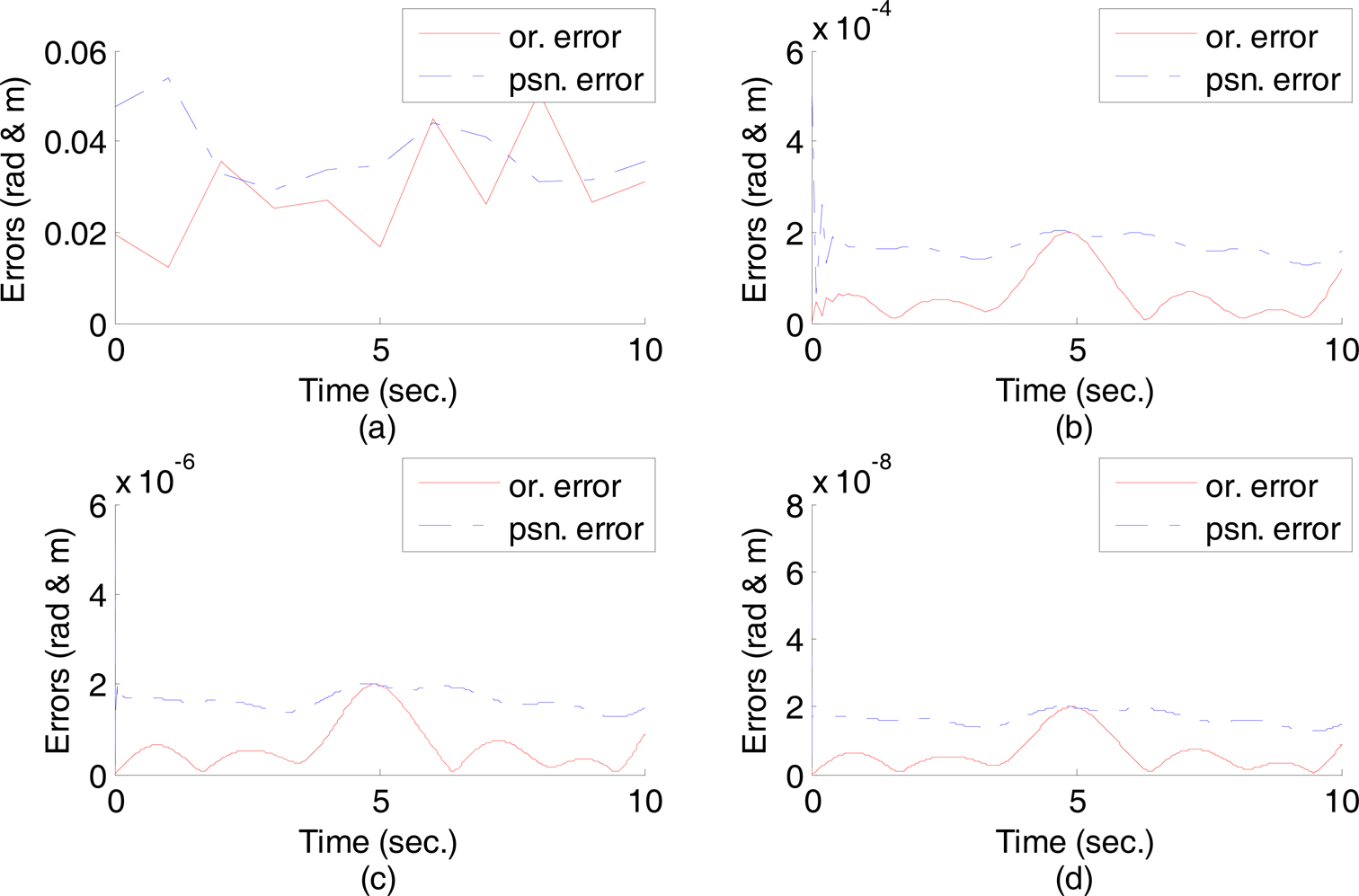
Total orientation and position errors (radian and meter) of the end effector for the Euler integration method and the sampling rates are (a) Δt = 1 s (b) Δt = 100 ms (c) Δt = 10 ms (d) Δt = 1 ms

Figure 10.

Total orientation and position errors (radian and meter) of the end effector for the Runge-Kutta 2 and the sampling rates are (a) Δt = 1 s (b) Δt = 100 ms (c) Δt = 10 ms (d) Δt = 1 ms

Figure 11.

Total orientation and position errors (radian and meter) of the end effector for the Runge-Kutta 4 and the sampling rates are (a) Δt = 1 s (b) Δt = 100 ms (c) Δt = 10 ms (d) Δt = 1 ms

Figure 12.

Total orientation and position errors (radian and meter) of the end effector for the Euler Trapezoidal Predictor & Corrector method and the sampling rates are (a) Δt = 1 s (b) Δt = 100 ms (c) Δt = 10 ms (d) Δt = 1 ms

Figure 13.

Total orientation and position errors (radian and meter) of the end effector for the fourth order Adams-Bashforth method and the sampling rates are (a) Δt = 1 s (b) Δt = 100 ms (c) Δt = 10 ms (d) Δ1 = 1 ms

Figure 14.

Total orientation and position errors (radian and meter) of the end effector for the fourth order Adams-Moulten method and the sampling rates are (a) Δt = 1 s (b) Δt = 100 ms (c) Δt = 10 ms (d) Δt = 1 ms

Table 1.

Running environment

Cpu	Cpu Memory	Operating System	Simulation Software
Intel Core2 Duo	2 GB	Windows	Matlab
2.2 GHz		XP	2009a

Note that simulation results are obtained for the desired trajectory which has 0.1 m/sec linear velocity and 0.2 rad/sec angular velocity.

Runge-Kutta 4

D. Multi-Step Numerical Integration Methods

Euler Trapezoidal Predictor & Corrector Method

Adams-Bashforth Methods (Fourth Order)

Adams-Moulton Methods (Fourth Order)

As it can be seen from the figures 9, 10, 11, 12, 13 and 14, the most accurate method is Runge-Kutta 4 and the least accurate method is Explicit Euler Integration. Explicit Euler Integration based solution gives fairly poor accuracy results in the trajectory tracking application. The results of this method can be seen in the figure 9. Small sampling rates, which increase the computational loads of the trajectory tracking algorithm, should be used to improve the accuracy of the numerical integration method and also to avoid the instability. As it can be seen from the figure 9 (a), Explicit Euler Integration based solution makes the system instable and errors get higher when the sampling rate is Δt = 1 sec. The Euler Trapezoidal Predictor & Corrector method also gives poor accuracy results in the trajectory tracking application. The result of this method can be seen in the figure 12. However, it has poor accuracy as Explicit Euler Integration; it is stable when the sampling rate is Δt = 1 sec. The other predictor & corrector based numerical integration method is Adams-Moulten. This method uses Adams-Bashforth algorithm for the prediction and Adams-Moulten algorithm for the correction. As it can be seen from the figures 13 and 14, both of these methods give quite accurate and stable results in the trajectory tracking application. However, Adams-Moulten based solution is more accurate and stable than Adams-Bashforth based solution. At last, Runge-Kutta based numerical integration results can be seen in the figures 10 and 11. As it can be seen from the figures, Runge-Kutta based numerical integration based solution gives very accurate and stable results. Also, the fourth order Runge-Kutta method (Runge-Kutta 4) gives the most stable and accurate numerical integration results. Runge-Kutta based numerical integration gives quite accurate results when the sampling rates are high. For instance, position errors of the end effector are about 10⁻⁶ for Runge-Kutta 2 and 10⁻⁸ for Runge-Kutta 4 when the sampling rate is 100 ms. High sampling rates improve the computational performance of the algorithm.

At or around the singular configurations of robot manipulator, Jacobian transformation generates high joint velocities which results in instability and large errors in the task space. The main reason of the large errors in the task space is that the differential kinematic based solution is the locally linearized approximation of the inverse kinematic problem and it is valid only for relatively small joint velocities. This case is explained clearly in the section of differential robot kinematics. Therefore, whatever the numerical integration method used task space errors will be increased at or around the singular configurations of the robot arm. However, accuracy results will be different in terms of the used numerical integration methods. The position and orientation errors around the singular configurations of robot arm can be seen in the figures 15 and 16.

Figure 15.

Total orientation and position errors (radian and meter) of the end effector around the singular configurations of robot arm for the Explicit Euler, Runge-Kutta 2 and Runge-Kutta 4 numerical integration methods. Sampling rate is Δt = 100 ms

Figure 16.

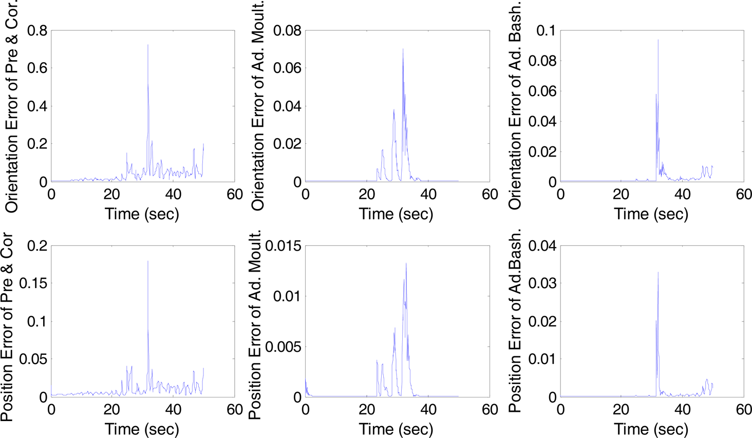
Total orientation and position errors (radian and meter) of the end effector around the singular configurations of robot arm for the Predictor & Corrector, Adams-Bashforth and Adams-Moulton numerical integration methods. Sampling rate is Δt = 100 ms

Figures 15 and 16 show the trajectory tracking errors around the singular configurations of robot arm using single and multi steps numerical integration methods respectively. As it can be seen from the figures 15 and 16, Runge-Kutta 4 numerical integration method gives the most accurate and stable results around the singular configurations of robot arm. However, the errors are still getting high around the singular configurations of robot arm even if Runge-Kutta 4 is used. Since, singularity does not depend on the used numerical integration method. It actually based on the configurations of the robot manipulator. Therefore, we should use different techniques such as avoiding singular configuration, robust inverse etc., to cope with the kinematic singularity problems. The results of the avoiding singular configuration method are shown in the figures 9, 10, 11, 12, 13 and 14. In this method, a trajectory, which does not suffer from kinematic singularity problems, is generated and the kinematic problem is solved by using this singularity free trajectory. Also, there are several robust inverse kinematic algorithms to cope with the kinematics singularity problem [36, 37]. Damped least squares method is one of the most widely used robust inverse kinematics algorithm [38, 39]. If we apply the robust inverse kinematics algorithm using the damped least squares method then, we get the errors around the singular configurations of robot arm as shown in the figures 17 and 18.

Figure 17.

Total orientation and position errors (radian and meter) of the end effector around the singular configurations of robot arm using Explicit Euler numerical integration method and damped least squares based robust inverse kinematics algorithm. Sampling rate is Δt = 100 ms

Figure 18.

Total orientation and position errors (radian and meter) of the end effector around the singular configurations of robot arm using Runge-Kutta 4 numerical integration method and damped least squares based robust inverse kinematics algorithm. Sampling rate is Δt = 100 ms

As it can be seen from the figures 17 and 18, robust kinematics algorithm using the damped least squares method gives satisfactory trajectory tracking results around the singular configurations of robot arm. Moreover, Runge-Kutta 4 based numerical integration methods gives more accurate results around the singular configurations of robot arm.

6. Conclusion

In this paper, we analyzed the performance of numerical integration methods in the trajectory tracking application of redundant robot manipulators. The performance of the trajectory tracking algorithm is drastically affected by the chosen numerical integration method. For instance, more accurate and more computationally efficient trajectory tracking algorithm can be obtained by changing the numerical integration methods. Even, the trajectory tracking algorithm may become instable due to the chosen numerical integration method. Here, we compared six different numerical integration methods with respect to computational efficiency and accuracy. Among these methods, Runge-Kutta and Adams methods give satisfactory results. When we compare the Runge-Kutta and Adams methods, Runge-Kutta based algorithms give more accurate and stable results however; they require extra computation. Thus, the Adams methods are more computationally efficient than Runge-Kutta methods. In the trajectory tracking application, Runge-Kutta based algorithms give quite satisfactory results when the sampling rates are high. As the sampling rates increase, computational load of the trajectory tracking algorithm decreases. However Runge-Kutta based algorithms require extra computations and have high computational load, the satisfactory results at high sampling rates may reduce even eliminate the computational efficiency disadvantages’ of this method.

References

Chang

P. H.

, “A Closed-Form Solution for Inverse Kinematics of Robot Manipulators with Redundancy”, IEEE Journal of Robotics and Automation, vol. RA-3, no. 5 Oct. 1987.

Yoshikawa

, “Analysis and Control of Robot Manipulators with Redundancy,” In Robotics Research–The First International Symposium, MIT Press, Cambridge, MA 1984 pp. 735–747.

Uchiyama

, “Study in Dynamic Control of Artificial Arm-Part I”, Trans. JSME, vol. 45, no. 391, pp 314–322, 1979.

Ping

Wei

and Luo

, “Real-Time Obstacle Avoidance for Redundant Robot”, IEEE International Conference on Mechatronics and Automation, pp. 223–228, Aug. 2009.

Cheni

Lin

, “Motion Planning of Redundant Robots”, Journal of Robotic Systems , 14(12), pp. 839–850, 1997.

Bertram

Kuffner

Dillmann

Asfour

, “An Integrated Approach to Inverse Kinematics and Path Planning for Redundant Manipulators”, IEEE, International Conference on Robotics and Automation (ICRA), pp. 1874–1879, May. 2006.

Siciliano

Khatib

, “Handbook of Robotics”, Springer, 2008.

Hasan

A.T.

Ismail

Hamouda

A.M.S

Aris

Marhaban

M.H.

Al-Assadi

H.M.A.A.

, “Artificial Neural Network-Based Kinematics Jacobian Solution for Serial Manipulator Passing through Singular Configurations”, Advances in Engineering Software , Vol.41, pp. 359–367, 2010.

Pashkevich

A. P.

Dolgui

A. B.

, “Kinematic Control of A Robot-Positioner System for Arc Welding Application”, Industrial Robotics: Programming, Simulation and Applications, pp. 702 Dec. 2006.

10.

Chiaverini

Siciliano

Egeland

, “Review of the Damped Least-Squares Inverse Kinematics with Experiments on an Industrial Robot Manipulator”, IEEE Transactions on Control System Technology , vol.2 pp. 123–134, 1994.

11.

Wolovich

W. A.

Elliott

, “A Computational Technique for Inverse Kinematics”, Proceedings of 23^rd Conference on Decision and Control, Dec. 1984.

12.

Caccavale

Chiacchio

Chiaverini

Siciliano

, “Experiments of Kinematic Control on a Redundant Robot Manipulator”, Laboratory Robotics and Automation , vol. 8, pp. 25–36, 1996.

13.

Wolovich

W. A.

Elliott

, “A Computational Technique for Inverse Kinematics”, Proceedings of 23^rd Conference on Decision and Control, Las Vegas, Dec. 1984.

14.

Angeles

, “Fundamentals of Robotic Mechanical Systems”, Springer, 2003.

15.

Tan

Wang

, “A Singularity-Free Motion Control Algorithm for Robot Manipulators - A Hybrid System Approach”, Automatica, (40), pp. 1239–1245, 2004.

16.

Fang

, “Study of Singularity Robust Inverse of Jacobian Matrix for Manipulator”, International Conference on Machine Learning and Cybernetics, Beijing, pp. 406–10, 2002, 32

17.

Nakamura

Hanafusa

, “Inverse Kinematic Solutions with Singularity Robustness for Robot Manipulator Control”, Journal of Dynamic Systems, Measurement and Control , Vol.108, pp.163–71, 1986.

18.

Wampler

C.W.

, “Manipulator Inverse Kinematic Solutions Based on Vector Formulations and Damped Least-Squares Methods”, IEEE Transactions on Systems, Man and Cybernetics, Vol.16, pp. 93–101, 1986.

19.

Balestrino

De Maria

Sciavicco

, “Robust Control of Robotic Manipulators”, International proceedings of the 9th IFAC world congress, Budapest, Vol.6, pp.80–85, 1984.

20.

Lin

Huang

, “Numerical Integration of Multibody Mechanical Systems Using Baumgarte's Constraint Stabilization Method”, Journal of the Chinese Institute of Engineers , vol. 25, no. 2, pp. 243–252 (2002)

21.

Sciavicco

Siciliano

, “Coordinate Transformation: A Solution Algorithm for One Class of Robots,” IEEE Transactions on Systems, Man and Cybenetics, vol. 16, pp. 550–559, 1986.

22.

Wampler

C.W.

Leifer

L.J.

, “Applications of Damped Least-Squares Methods to Resolved-Rate and Resolved-Acceleration Control of Manipulators,” Journal of Dynamic Systems, Measurement and Control, vol. 110, pp. 31–38, 1988.

23.

Chiacchio

Chiaverini

Sciavicco

, and Siciliano

, “Closed-Loop Inverse Kinematics Schemes for Constrained Redundant Manipulators with Task Space Augmentation and Task Priority Strategy”, Int. Journal of Robotics Research , vol. 10, pp. 410–425, 1991.

24.

Ueberhuber

C. W.

, “Numerical Computation 2: Methods, Software, and Analysis”, Springer, 1997.

25.

Schilling

R. J.

, “Applied Numerical Methods for Engineers”, Brooks/Cole 2002.

26.

Heinbockel

J. H.

, “Numerical Methods for Scientific Computing”, Trafford Publishing, July, 2006.

27.

Krommer

A. R.

, “Numerical Integration on Advanced Computer Systems (Lecture Notes in Computer Science)”, Springer, Oct., 1994.

28.

Voronin

S. M.

, “On Numerical Integration Algorithms”, Izv. Maht,. vol. 60, pp. 887–891 (1996),

29.

Cheah

C.C.

Hirano

Kawamura

Arimoto

, “Approximate Jacobian Control for Robots with Uncertain Kinematics and Dynamics”, IEEE Transactions on Robotics and Automation , vol.19, no. 4, Aug. 2003.

30.

Spong

M.W.

Hutchinson

Vidyasagar

, “Robot Modeling and Control”, Wiley, 2005.

31.

Craig

J.J.

, “Introduction to Robotics: Mechanics and Control”, 3rd edition., Prentice Hall, 2006.

32.

Rodriguez

K-Delgado

Jain

, “A Spatial Operator Algebra for Manipulator Modeling and Control”, International Journal of Robotics Research , vol. 10, pp. 371–381, Aug. 1991.

33.

Afshari

Meghdari

, “New Jacobian Matrix and Equations of Motion for a 6-DOF Cable-Driven Robot”, International Journal of Advanced Robotic Systems, vol.4, no.1, 2007.

34.

Katsiaris

P. T.

Artemiadis

P. K.

Kyriakopoulos

K. J.

, “Modelling Anthropomorphism in Dynamic Human Arm Movements”, International Conference on Intelligent Robot and Systems (IROS), Taipei, pp. 3507–3512, 18–22 Oct. 2010.

35.

Lohmeier

Buschmann

Ulbrich

, “System Design and Control of Anthropomorphic Walking Robot LOLA ”, IEEE Transactions on Mechatronics, vol. 14, pp. 658–666, Dec. 2009.

36.

Mukundan

, “A Robust Inverse Kinematics Algorithm for Animating a Joint Chain”, International Journal of Computer Applications in Technology , vol. 34, pp.303–308, March 2009.

37.

Foret

Xie

Fontaine

J.G.

, “Bordered Matrix for Singularity Robust Inverse Kinematics: A Methodological Aspect”, Proceedings of International Conference on Robotics and Automation , vol. 3, pp. 3013–3019, 24–28 Apr. 2000.

38.

Deo

A. S.

Walker

I. D.

, “Overview of damped least-squares methods for inverse kinematics of robot manipulators”, Journal of Intelligent and Robotic Systems , vol. 14, pp. 43–68, 1995.

39.

Buss

S.R.

Kim

J.S.

, “Selectively Damped Least Squares for Inverse Kinematics”, Journal of Graphics GPU & GameTools , vol. 10, pp. 37–49, March 2008.

Performance Analysis of Numerical Integration Methods in the Trajectory Tracking Application of Redundant Robot Manipulators

Abstract

Keywords

1. Introduction

2. Differential Robot Kinematics

References