Explicit Dynamic Formulation for n-R Planar Manipulators with Frictional Interaction between End-Effecter and Environment

Abstract

This paper includes modeling and dynamic analysis of the planar manipulators which consist of n revolute joints and its end-effecter may possess a frictional contact with an arbitrary surface. The dynamic analysis has been done by using the Lagrangian method. The main contribution of this work is presenting the equations of motion of the system in an explicit and straightforward manner. To this end, the absolute angles of the links are chosen as the generalized coordinates to constitute the Lagrangian, and by this way the Coriolis acceleration terms included the product of the joint velocities, will be hidden in structure of the equations of motion. It is very interested in the simplified results that show a clear conformity with the interpretations of the Euler's equation of motion of the rigid body. In following, the results are applied to a case study model to explain the deriving the equations of motion by our formulation. An inchworm robot included an articulated mechanism is considered to this end.

1. Introduction

Recently, robotic manipulators are widely used to help in dangerous and monotonous industrial jobs to improve productivity and accuracy. This has caused the emergence of an area of research in the field of manufacturing automation, and robotics due to a wide spectrum of applications starting from simple pick and place operations of an industrial robot to micro-surgery, maintenance of nuclear plants, and space robotics [1].

Controlling of a high precision robot is severely limited to possessing an exact and yet simple dynamic model for it to be used by a control law. But, complexity of robotic manipulator dynamics included generally highly coupled and nonlinearity equation is a problem that challenges all researches and engineers that investigate on this field. This problem is emphasized for redundant manipulators that possess at least one degree-of-freedom (DOF) more than the required one for their particular positioning task [2,3]. The extra DOFs are able to enhance the skill and flexibility of the entire robotic system, and hence are able to increase the operational use and to obtain the maximum use of the robotic workspace. Moreover, robotic manipulators can use the redundancy in their benefit to avoid their joint limits and the obstacles in the workspace, while still reaching a desired end-effecter pose in the task space [4,5]. Avoidance of and passing through singularities is another major aspect that makes the use of redundancy in manipulators very preferable [6,7].

However, increasing the redundancy causes the increasing the complexity of kinematic and dynamic analysis and so controlling the robotic system. Thus, investigating on variety aspects of redundant manipulators has become the one of the most important research subjects in today robotics. For example, many efforts for solving of the inverse kinematics problem of redundant robotics have been done by various methods [8–12]. Also, several classical and heuristic algorithms are applied to develop the path planning for redundant manipulators and its optimization based on their kinematic or dynamic parameters. Using the B-splines [7,13], defining the potential field [14], applying the perturbation [15], Integrated [16], variational [17], and fractional [18] approaches, besides of neuro-fuzzy [19] and evolutionary [20] or genetic algorithms [21] are examples of variety techniques related to trajectory planning for redundant manipulators analysis.

Controlling the end-effecter to track the planned path is the ultimate aim of the robotic manipulators. But, a theoretical approach to the control problem usually incorporates a dynamic model of a mechanism. Thus, a variety of dynamic formulations and control algorithms have been also developed to improve the robotic kinematic and dynamic model quality, computational speed, control accuracy and robustness, theoretical generalizability and the breadth and depth of physical insight [22–27]. For the evaluation of theoretical results it would be of benefit to have dynamic models of mechanisms with arbitrary number of degrees of freedom. Thus, this paper intends to develop a new dynamic formulation for n-R planar manipulators that are the most used case study model of redundant manipulators.

From the point of view of classical mechanics, deriving the equations of motion of a rigid-link manipulator is usually regarded as a straightforward procedure: once a suitable set of generalized coordinates and reference frames have been chosen, what remains is to apply either Tagrange's formulation or Newton and Euler's equations to obtain the differential equations of motion [28]. Here, Tagrangian method dynamic analysis is used to constitute our new formulation, and absolute link angles are chosen as generalized coordinates to describe the configuration of the robotic arm. The model is generally considered so as the end-effecter can possess a constant connection with a frictional surface. Our main aim is presenting the closed-form equations of motion in an explicit and straightforward manner.

In next sections the problem description is done and then kinematic and dynamic analysis of model with physical interpretation of formulas is presented. In following, a robotic inchworm with an articulated mechanism is modeled as a manipulator, and obtained results are applied to simulate it, so as required joint torques for performing a certain gait pattern are achieved. Finally, results of the simulation of one step of the motion course are presented.

2. Problem Description

As mentioned above the main contribution of this paper is derivation of the explicit and closed-form motion equations for n–R planar manipulators in a general condition for the interaction between the end-effecter and environment. In particular we are interested to simplify the structure of the motion equations by hiding the Coriolis acceleration effects including product of the joint velocities. On this way, without reducing the generality of the problem, the equations are constituted in a straightforward manner and physical interpretation of them will be explicit. To this end the absolute link angles, φ_is, measured with respect to positive direction of horizontal axis, are chosen as a set of generalized coordinates instead of choosing the relative joint angles as one. In according to Figure 1, it is clear that for i = 1 … n we have:

${\phi }_i= {\sum }_{j=1}^i{\theta }_j{=\phi }_{i-1}+ {\theta }_i\mathrm{ },\mathrm{ }\mathrm{w}\mathrm{i}\mathrm{t}\mathrm{h}\mathrm{ } {\phi }_0=0.$

(1)

Figure 1.

Manipulator model possessing interaction between end-effecter and environment.

Moreover, as shown in Figure 2, a set of body frames are attached to links and each of them is recognized by number of its link. The origin of the each frame is coincided to hind joint axis of the link and its X axis is aligned with link length. Thus, the relative acceleration of the link frame {p+1} - that is coincident with point P_p+1 in the Figure 2 - with respect to its posterior neighbor link frame {p} is calculated and denoted as follows:

$\begin{array}{l}{\hspace{0.17em}}^p{\hspace{0.17em}}_{\mathbf{a}p+1\mathbf{r}\mathbf{e}\mathbf{l}}^{\hspace{0.17em}}= -l_p\left({\ddot{\phi }}_p\sin {\phi }_p+{\dot{\phi }}_p^2\cos {\phi }_p\right)\mathbf{i}\\ +l_p\left({\ddot{\phi }}_p\cos {\phi }_p-{\dot{\phi }}_p^2\sin {\phi }_p\right)\mathbf{j}\end{array}$

(2)

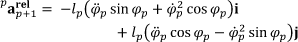
What is appeared explains that relative acceleration contains the only tangential and centripetal accelerations terms. However, as a matter of fact, the terms corresponded to Coriolis accelerations have been hidden in the squares of the angular velocity of the links calculated by Eq. 1, too. Thus, by eliminating the terms included the product of the joint velocities from the motion equations; its structure will be simplified, particularly in higher order DOF.

It's also worth calculating the moment of calculated relative acceleration with respect to an arbitrary point P _q -which can be origin of link frame {q} - as following:

$\begin{array}{l}{\mathrm{I}}_q\times {\hspace{0.17em}}^p{\mathrm{a}}_{p+1}^{\mathbf{r}\mathbf{e}\mathbf{l}}=l_q(\text{cos}{\phi }_q\mathbf{i}+\text{sin}{\phi }_p\mathbf{j})\times {\hspace{0.17em}}^p{\mathbf{a}}_{p+1}^{\mathbf{r}\mathbf{e}\mathbf{l}}\hfill \\ =I_p{l}_q({\ddot{\phi }}_p\text{cos}({\phi }_p-{\phi }_q)\hfill \\ -{\dot{\phi }}_p^2\text{sin}({\phi }_p-{\phi }_q))\hfill \end{array}$

(3)

Henceforth, this quantity is denoted by function M(p,q) which is defined in an abbreviated form as:

$\mathrm{M}\left(p,q\right)=\mathrm{ }{l}_p{l}_q\left({\ddot{\phi }}_p C_{pq}-{\dot{\phi }}_p^2{S}_{pq}\right)$

(4)

where l _q is moment arm length.

Figure 2.

Relative acceleration between two sequential link frames its moment with respect to link point Pq.

3. Dynamic Analysis

In this section we pay attention to derivation of the equations of motion for our system based on energy method, i.e. Lagrangian formulation. But before getting into this subject, let us mention that alternative method to derive the equation of motion is Newton-Euler formulation based on Newton's Second Law which relates force and momentum, as well as torque and angular momentum. This formulation is usually performed by recursive algorithms, and the resulting equations involve workless constraint forces, which must be eliminated. Thus, arithmetic operations are needed to separate the input joint torques from the constraint forces and moments to derive the closed-form dynamic equations. Specially, in the Newton-Euler formulation, the equations are not expressed in terms of independent variables, and do not include input joint torques explicitly. Briefly, by using this method the equations of motion are not appeared in an appropriate form for use in dynamic analysis and control design [29].

Instead, Lagrangian formulation, which is an analytical method for deriving the governing equations, describes the behavior of a dynamic system in terms of work and energy stored in the system rather than of forces and moments of the individual members involved. In this method, the constraint forces involved in the system are automatically eliminated in the formulation of Lagrangian dynamic equations, and the closed-form dynamic equations can be derived systematically in any coordinate system. Now, by knowing these facts, we follow the derivation of the equations of motion based on Lagrangian formulation.

As discussed in robotic literatures, joint angular displacements Θ are a complete and independent set of generalized coordinates that locate the whole robot mechanism. However, as mentioned in previous section, this choice causes that the relative Coriolis accelerations are appeared in the equations of motion, and so the complexity of equations increases. Therefore, we select link angles Φ as an independent set of generalized coordinate for describing our system and constituting the Lagrangian formulation.

Let T and V denote the total kinetic and gravity potential energies of system. Thus, using the Lagrangian formulation, equations of motion of the dynamic system are given by:

$\frac{d}{dt}\left(\frac{\partial T}{\partial {\dot{\phi }}_k}\right)- \frac{\partial T}{\partial {\phi }_k}+\frac{\partial V}{\partial {\phi }_k}=Q_k$

(5)

where the total kinetic energy of system is associated with linear velocity of centroid, v̄ _p , and angular velocity, φ̇ _p , of each individual link, and calculated by:

$T=\frac{1}{2}{\sum }_{p=1}^n\left(m_p{\bar{v}}_p^2+ {\bar{I}}_p{\dot{\phi }}_p^2\right)$

(6)

where the length, mass, and moment of inertia about centroid of p^th link are denoted by l _p , m _p , and Ī _p , respectively. For simplification, position of centroid of each link is considered to be at its midpoint, and to have the body like a bar with Ī _p = m _p l² _p /12. v̄² _p is also given by:

${\bar{v}}_p^2={\stackrel{-}{\mathbf{v}}}_p\mathbf{ }.\mathbf{ } {\stackrel{-}{\mathbf{v}}}_p= \frac{l_p^2}{4}{\dot{\phi }}_p^2+{\sum }_{i=1}^p{\sum }_{j=1}^{p-1}{l}_i{ l_{j }{\dot{\phi }}_i \dot{\phi }}_j \mathrm{c}\mathrm{o}\mathrm{s}({\phi }_i-{\phi }_j)$

(7)

Furthermore, the gravity potential energy of system is equal to;

$V={\sum }_{p=1}^n{m}_{p}g{\bar{h}}_p=g{\sum }_{p=1}^n{m}_p\left({\sum }_{i=1}^p{l}_i\mathrm{s}\mathrm{i}\mathrm{n}{\phi }_i-\mathrm{ }\frac{l_p}{2}\mathrm{ }\mathrm{s}\mathrm{i}\mathrm{n}{\phi }_p\right)\mathrm{ }$

(8)

Moreover, Q _k is the generalized force corresponding to the generalized coordinate φ _k . Generally, this dynamic system includes two set of nonconservative terms; first, joint torques acted on the links that considered as inputs, and second, constraint forces that arise from interaction between end-effecter and environment. It's worth noting that when end-effecter is constrained to track a certain path, one degree of freedom of the system is decreased. Then the selective generalized coordinates won't be independent set and are related by constraint equation. Thus, two methods are possible for using the constrained generalized coordinates; using the Lagrange multipliers as well as contributing the work done by reaction forces. Each one of these methods involves a set of unknown parameters in equations; unknown Lagrange multipliers as well as unknown reaction forces values, which are equivalent to each other. In fact, the physical meaning of Lagrange multipliers is the same reaction forces values. Since end-effecter in our system is constrained to remain in contact with its interaction surface, the explained phenomena occurs. Furthermore, because the friction reaction is not really arisen from a constraint on the motion, using the Lagrange multipliers method fails. Then, we should calculate the generalized forces by considering the all actions on the system.

Let N and f are the normal and frictional reaction forces act on the tip of the end-effecter. The curve of the connection points is also given by f(x,y) = 0. By considering the Coulomb friction model, and noting that the friction force acts in direction opposite to the velocity vector, the resultant reaction force is achieved by:

$\mathbf{F}=-\left(f{\mathbf{e}}_{\mathbf{t}}+N{\mathbf{e}}_{\mathbf{n}}\right)=-N\left(\bar{\mu }{\mathbf{e}}_{\mathbf{t}}+{\mathbf{e}}_{\mathbf{n}}\right)=-N\left(\left(\bar{\mu }+y^{\text{'}}\right)\mathbf{i}-\left(1-\bar{\mu }{y}^{\text{'}}\right)\mathbf{j}\right)/{\left(1+{y^{\text{'}}}^2\right)}^{\frac{1}{2}}$

(9)

where μ̅ = μ sign(v _tip . e_t), and μ is friction coefficient. The virtual work done by F is equal to:

$\begin{array}{c}\delta W_{\mathbf{F}}=\mathbf{F}.\delta {\mathbf{P}}_{p+1}= \frac{N}{\sqrt{1+{y\text{'}}^2}}\left(\left(\bar{\mu }+y^{\text{'}}\right)\sum _{p=1}^n{l}_p\mathrm{s}\mathrm{i}\mathrm{n}{\phi }_p\delta {\phi }_p+\left(1-\bar{\mu }{y}^{\text{'}}\right)\sum _{p=1}^n{l}_p\mathrm{c}\mathrm{o}\mathrm{s}{\phi }_p\delta {\phi }_p\right)=\\ N \sum _{p=1}^n\frac{l_p}{\sqrt{1+{y\text{'}}^2}}\left(\left(\bar{\mu }+y^{\text{'}}\right)sin{\phi }_p+\left(1-\bar{\mu }{y}^{\text{'}}\right)cos{\phi }_p\right)\delta {\phi }_p\\ \equiv N\sum _{p=1}^n{\lambda }_p\delta {\phi }_p\end{array}$

(10)

As it's defined, the λ _p is the same constraint coefficient associated with Lagrange multiplier – that here is N – corresponding to p^th generalized coordinate, φ _p .

In addition, the virtual work done by input joint torques, i.e. τ, is calculated as:

$\delta W_{\mathbf{\tau }}=\mathbf{\tau }.\delta \mathbf{\Theta }= \sum _{p=1}^n{\tau }_p\delta \left({\phi }_p-{\phi }_{p-1}\right)=\sum _{p=1}^n\left({\tau }_p-{\tau }_{p+1}\right)\delta {\phi }_p$

(11)

Figure 3.

Inchworm mode locomotion, performed by an articulated robot.

Therefore, the total virtual work done by input joint torques and reaction forces is:

$\delta W=\delta W_{\mathbf{\tau }}+\delta W_{\mathbf{F}}={\sum }_{p=1}^n\left({\tau }_p-{\tau }_{p+1}+{\lambda }_{p}N\right)\delta {\phi }_p={\sum }_{p=1}^n{Q}_p\delta {\phi }_p$

(12)

Now, by substituting the results into the Lagrange Equation 5, and simplifying the equation, it's obtained – For briefing the details of calculations are cited in Appendix.

$\begin{array}{c}\left(\mathrm{ }\frac{m_k}{2}+\sum _{p=k+1}^n{m}_p\right)\mathrm{ }g{\mathrm{ }l}_k\mathrm{c}\mathrm{o}\mathrm{s}{\phi }_k+\\ \sum _{p=k+1}^n{m}_p\left(\frac{1}{2}\mathrm{M}\left(p,k\right)+\sum _{i=1}^{p-1}\mathrm{M}\left(i,k\right)\right)+\frac{1}{2}{m}_k\sum _{j=1}^{k-1}\mathrm{M}\left(j,k\right)+\\ +I_k{\ddot{\phi }}_k={\tau }_k-{\tau }_{k+1}+{\lambda }_{k}N,\mathrm{ } k\mathrm{ }=\mathrm{ }1\dots n\end{array}$

(13)

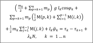
As can be seen, the equations of motion include the summation of M(.,.) function multiplied by a link mass. It's said that M(p,q) function is, in fact, the moment of relative acceleration between the two ends of the link p, with respect to origin of another link frame {q}. Then, the summation ∑^p-1_i=1 M(i,q) means moment of absolute acceleration of the behind end of the p^th link with respect to the P_q. Now, by considering the figures 2, and isolating the link p, assume that it's desired to apply the Euler's equation for balancing the moments of the inertial effects and exerted forces on the p^th link, with respect to the moving point P _p . Thus, Eq. 13 explains that the moments of the weight of the all links that are ahead of the P _p , add to the moment of the effect of inertial forces of the same links that appears as an internal joint force at point P_p+1, whit respect to the P _p , add to moment of the inertial effects of the link p itself, included by the moment of the inertial force at the centroid and inertial moment, about the moving point P _p , are equal to the tourqes exerted by actuators plus to the moment of reaction forces transmitted through linkage to the point P_p+1. It's also noting that moment of internal joint force at P _p is zero. That is the equations are derived by Lagrangian method are exactly compatible with Eulerian physical interpretation.

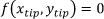
Moreover, the presented equations of motion include the n independent relations and n+1 unknown parameters, i.e. generalized coordinate set in addition to normal reaction force, N. In fact, the equation of tracked path is the completing relation to solve those equations. Thus, it should be hold as:

$f\left(x_{tip},y_{tip}\right)=0$

(14)

It's obvious that if the friction is neglectable it is enough to take μ̅ = 0. But the normal reaction on the surface is still the force that permits the end-effecter to take no exceeding into the surface. However, if it's desired that end-effecter tracks the certain path with the same function as given by Eq. 14, then no reaction force will exist. In these cases it is also taken μ̅ = 0 for evaluating the λ _k , but the N coefficient is not null value, and play role of the Lagrange multiplier instead of normal reaction; as it can be well imagine that a virtual force – instead of a visual force – is existed that causes the end-effecter remains on specified path. Finally, if the end-effecter is not constrained in motion then the manipulator possesses the full n degrees-of-freedom and it's taken N = 0.

Expect for simulating the manipulators, the equations of motion may be applied to evaluate the torque that required by each actuator to be followed a certain planned path by end-effecter. In fact, in these problems the time histories of the joint angles – and subsequently, for the link angles – are specified and controlling the robot arm is desired. Hence, the torques are unknowns, instead of the generalized coordinates, i.e. Φ. It's nothing that if end-effecter is constrained on motion, the reaction force – whether visual or virtual – is another unknown, and obtained by a constraint relation. Moreover, if end-effecter possesses a connection with environment, force control problem should add to position control to perfect the control problem.

4. Modelling of an Inchworm Robot

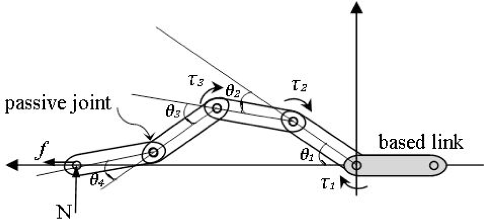
The inchworm mode locomotion has been defined and modeled in our previous work [30,31]. As shown in Figure 3, the advancement of the reptile robot is achieved by propagation of a wave through its linkage in four steps. As shown in Figure 4, the motion of the mobile robot in each step may be considered as the motion of a simple manipulator with a non-moving based. In fact it's supposed that friction between the non-moving links and ground is so much that causes these links don't slide.

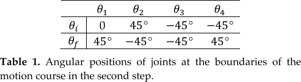
Now, we intend to take a case study approach to illustrate the simplicity of derivation and the structure of equations of motion that are derived by using the Eq. 13. Let us choose the second step of the motion course for dynamic analyzing. In this step, robot changes its configuration from state 1 to state 2, as shown in Figure 3. The angular positions of joints at beginning and end of the motion is given by table 1. Moreover, it's desired that the joint velocities at the same times become zero. Besides, in order to avoid redundancy in system, the last joint in sub-mechanism is taken to be passive, i.e. τ₄ = 0.

Figure 4.

One step of the motion course of the inchworm robot.

Table 1.

Angular positions of joints at the boundaries of the motion course in the second step.

	θ1	θ2	θ3	θ4
θ i	0	45°	-45°	-45°
θ f	45°	-45°	-45°	45°

The inchworm robot problem is a case in which the motion pattern is specified, in other words, the time history of angular position of joints is known, and it is desired to obtain the required torques to perform the locomotion. In this study it is considered that the each joint follows a linear function with parabolic blends as its time history. The velocity at the end of the blend region is chosen equal to the velocity of the linear section so that the entire path is continuous in position and velocity. It's also assumed that the parabolic blends both have the same duration; therefore, the same constant acceleration is used during both blends [32]. By taking the total and blends durations are T sec. and 0.1 T sec., respectively, the trajectory of the each active joint motion is given by:

$\theta \left(t^{*}\right)=\left\{\begin{array}{c}5\omega {t^{*}}^2+{\theta }_i\\ \omega \left(t^{*}-0.05\right)+ {\theta }_i\\ -5\omega \left({t^{*}}^2-2t^{*}+1\right)+{\theta }_f\end{array}\begin{array}{c}0\le t^{*}\le 0.1\\ 0.1\le t^{*}\le 0.9\\ 0.9\le t^{*}\le 1\end{array}\right.$

(15)

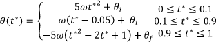
where, ω = (θ _f - θ _i )/(1 - 0.1), t* = t/T, and θ _t and θ _f for each joint is given in table 1.

It's noting that, in general, the trajectory of the last (passive) joint should be calculated by considering the geometrical constrain of the system; that is permanent connection between the tip of the last link and ground. It causes that the mechanism has a close-loop kinematic chain; that is:

${\sum }_{i=1}^4{l}_i\mathrm{s}\mathrm{i}\mathrm{n}{\phi }_i=0$

(16)

Thus, the angular position and its time derivates of passive joint can be calculated by:

$\begin{array}{c}{\theta }_4=-{\phi }_3-{\mathrm{s}\mathrm{i}\mathrm{n}}^{-1}\left(\sum _{i=1}^3\mathrm{s}\mathrm{i}\mathrm{n}{\phi }_i\right) \left(a\right)\\ {\dot{\theta }}_4=-{\dot{\phi }}_3-\frac{1}{\mathrm{c}\mathrm{o}\mathrm{s}{\phi }_4}\sum _{i=1}^3{\dot{\phi }}_i\mathrm{c}\mathrm{o}\mathrm{s}{\phi }_i \left(b\right)\\ {\ddot{\theta }}_4={\dot{\phi }}_4\mathrm{t}\mathrm{a}\mathrm{n}{\phi }_4-{\ddot{\phi }}_3-\frac{1}{Cos{\phi }_4}\left(\sum _{i=1}^3{\ddot{\phi }}_i\mathrm{c}\mathrm{o}\mathrm{s}{\phi }_i-\sum _{i=1}^3{\dot{\phi }}_i^2\mathrm{s}\mathrm{i}\mathrm{n}{\phi }_i\right) \left(c\right)\end{array}$

(17)

Now, by considering identical links for robot, (i.e. m _k = m,l _k = l, and I _k = I ≡ ml²/3, k = 1,2,3,4), and using the Eq. 13, the equations of motion of the mechanism are obtained as follows:

$\begin{array}{c}\frac{m{l}^2}{6}\left(\begin{array}{cccc}20& {15C}_{12}& {9C}_{13}& {3C}_{14}\\ {15C}_{12}& 14& {9C}_{23}& {3C}_{24}\\ {9C}_{13}& {9C}_{23}& 8& {3C}_{34}\\ {3C}_{14}& {3C}_{24}& {3C}_{34}& 2\end{array}\right)\left(\begin{array}{c}{\ddot{\phi }}_1\\ {\ddot{\phi }}_2\\ {\ddot{\phi }}_3\\ {\ddot{\phi }}_4\end{array}\right)\\ +\frac{m{l}^2}{6}\left(\begin{array}{cccc}0& {15S}_{12}& {9S}_{13}& {3S}_{14}\\ {-15S}_{12}& 0& {9S}_{23}& {3S}_{24}\\ {-9S}_{13}& {-9S}_{23}& 0& {3S}_{34}\\ {-3S}_{14}& -{3S}_{24}& {-3S}_{34}& 0\end{array}\right)\left(\begin{array}{c}{\dot{\phi }}_1^2\\ {\dot{\phi }}_2^2\\ {\dot{\phi }}_3^2\\ {\dot{\phi }}_4^2\end{array}\right)\\ \frac{+mgl}{2}\left(\begin{array}{c}{7\mathrm{c}\mathrm{o}\mathrm{s}\phi }_1\\ 5{\mathrm{c}\mathrm{o}\mathrm{s}\phi }_2\\ {3\mathrm{c}\mathrm{o}\mathrm{s}\phi }_3\\ \mathrm{c}\mathrm{o}\mathrm{s}{\phi }_4\end{array}\right)=\left(\begin{array}{cccc}1& -1& 0& 0\\ 0& 1& -1& 0\\ 0& 0& 1& -1\\ 0& 0& 0& 1\end{array}\right)\left(\begin{array}{c}{\tau }_1\\ {\tau }_2\\ {\tau }_3\\ 0\end{array}\right)+\left(\begin{array}{c}{\lambda }_1\\ {\lambda }_2\\ {\lambda }_3\\ {\lambda }_4\end{array}\right)N\end{array}$

(18)

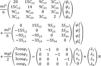
where λ _i = l(cosφ _i + μ̅sinφ _i ). This system of equations can be solved for the required torques to have a specified motion in joint space same as given by Eq. 15. Alternatively, they may be regarded as a set of non-linear coupled differential equations for joint coordinates in situation in where the torques are specified.

The interesting point is that the structure of the equations of motion is generally appeared in the simple form as:

$\mathrm{A}\left(\mathbf{\Phi }\right)\mathrm{ }\ddot{\mathbf{\Phi }}+\mathrm{B}\left(\mathbf{\Phi }\right)\mathrm{ }{\dot{\mathbf{\Phi }}}^2+\mathbf{G}\left(\mathbf{\Phi }\right)=\mathrm{E}\mathrm{ }\mathbf{\tau }+\mathbf{\lambda } N$

(19)

where symmetric matrix A and skew–symmetric matrix B are matrices of inertial effects associated with tangential and centripetal accelerations, respectively, related together by:

$\left[b_{ij}\right]=\frac{\partial }{\partial {\phi }_j}\left[a_{ij}\right]$

(20)

Also, G is the vector of gravity terms and E is the difference matrix. It should be noted that all the A, B and G matrices are only dependent on configuration state of the arms in each instant, i.e. Φ(t).

Here, by determining the dynamic characteristics of the arms, the system of Eqs. 18 can be solved for required torques and normal reaction force N. Generally, it can be also done by dimension–less analogy. To this aim both sides of the Eq. 18 are divided by mgl. Then, the equation is turned to:

$\frac{1}{{\omega }_n^2}{\mathrm{A}}^{\mathrm{*}}\left(\mathbf{\Phi }\right)\mathrm{ }\ddot{\mathbf{\Phi }}+\frac{1}{{\omega }_n^2}{\mathrm{B}}^{\mathrm{*}}\left(\mathbf{\Phi }\right)\mathrm{ }{\dot{\mathbf{\Phi }}}^2+{\mathbf{G}}^{\mathbf{*}}\left(\mathbf{\Phi }\right)=\mathrm{E}\mathrm{ }{\mathbf{\tau }}^{\mathbf{*}}+{\mathbf{\lambda }}^{\mathbf{*}} N^{*}$

(21)

where ω² _n = g/l, A* = A/ml², B* = B/ml², G* = G/mgl, τ* = τ/mgl, λ* = λ/l, and N* = N/mg.

But still, quantities link length, gravity acceleration, and friction coefficient need to be known in order to simulate the robotic inchworm. These are regarded as 0.14 m, 9.81 m/s^2 and 0.4, respectively.

The results obtained by simulation are depicted in following figures. The required torque to actuate each one of joints is shown in Figure 5. The normal reaction and horizontal velocity of the tip of the end-effecter, interacting with environment, are shown in figures 6 and 7. The snapshots of the motion in the second step, according to mentioned trajectories, are also shown in Figure 8.

As shown in Figure 5 and 6, the torque curves are broken at t* = 0.1 and 0.9 sec., because of non-continuity of joints accelerations at boundaries of parabolic blends of trajectories. They are also broken at t* = 0.5 sec., because of passing through a singular position. This singularity can be seen in middle picture of snapshots.

Figure 5.

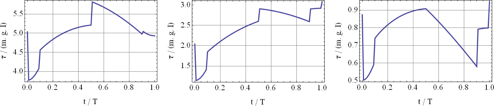
Required torque to actuate the first, second, and third joint.

Figure 6.

Normal reaction at tip of end-effecter

Figure 7.

horizontal velocity of tip of end-effecter

Figure 8.

Snapshots of the second step of the motion course.

5. Conclusion

This paper presents a new formulation in dynamic analysis of a planar manipulator consisting of multiple revolute joints with a frictional contact between the end-effecter and the environment surface. The dynamic analysis was based on Lagrangian method and equations of motion of the system were represented in an explicit and straightforward manner. The complexity correlated by Coriolis acceleration didn't appear in this new formulation. Moreover, this formulation demonstrated a clear conformity with the interpretations of the Euler's equation of motion of the rigid body. In following, as a case study approach, a crawling locomotion pattern which is performed by an articulated mechanism was modeled as a mobile manipulator. Especially, the required torques for performance of one step of the motion course are calculated by using the derived formulation. Finally, the results of simulation were shown.

This formulation can be developed for a mobile manipulator. It can also be regarded that axis of the first revolute joint in the robotic mechanism is orthogonal to other joint axes. The most importance of this formulation is in the identifying the robotic system; because of the simplicity of its structure that included the least independent parameters associated with characteristics of the arms. We intend to pay attention to these ideas in future works.

Appendix

Calculating of the total kinetic energy is done as follows:

$\begin{array}{c}T=\frac{1}{2}\sum _{p=1}^n\left(m_p{\bar{v}}_p^2+ {\bar{I}}_p{\dot{\phi }}_p^2\right)= \frac{1}{2}\sum _{p=1}^n\left(m_p\left(\frac{l_p^2}{4}{\dot{\phi }}_p^2+\sum _{i=1}^p\sum _{j=1}^{p-1}{l}_i{ l_{j }{\dot{\phi }}_i \dot{\phi }}_j\cos \left({\phi }_i-{\phi }_j\right)\right)+ {\bar{I}}_p{\dot{\phi }}_p^2\right)= \\ \frac{1}{2}\sum _{p=1}^n\left(m_p\frac{l_p^2}{4}+{\bar{I}}_p\right){\dot{\phi }}_p^2+\frac{1}{2}\sum _{p=1}^n{m}_p\sum _{i=1}^p\sum _{j=1}^{p-1}{l}_i{ l_{j }{\dot{\phi }}_i \dot{\phi }}_j\cos \left({\phi }_i-{\phi }_j\right)\\ \equiv \frac{1}{2}\sum _{p=1}^n{I}_p{\dot{\phi }}_p^2+ \frac{1}{2}\sum _{p=1}^n{m}_p{H}_p^2\end{array}$

(A1)

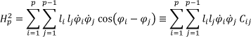
where H² _p is introduced as:

$H_p^2=\sum _{i=1}^p\sum _{j=1}^{p-1}{l}_i{l}_j{\dot{\phi }}_i{\dot{\phi }}_j\mathrm{ }\mathrm{c}\mathrm{o}\mathrm{s}\left({\phi }_i-{\phi }_j\right)\equiv \sum _{i=1}^p\sum _{j=1}^{p-1}{l}_i{l}_j{\dot{\phi }}_i{\dot{\phi }}_j\mathrm{ }{C}_{ij}$

(A2)

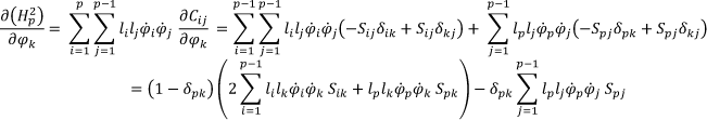
Thus required derivatives of H² _p are calculated as following:

$\begin{array}{c}\frac{\partial \left(H_p^2\right)}{\partial {\dot{\phi }}_k}=\mathrm{ }\sum _{i=1}^p\sum _{j=1}^{p-1}{l}_i{l}_j\left({\dot{\phi }}_i{\delta }_{jk}+{\dot{\phi }}_j{\delta }_{ik}\right)\mathrm{ }{C}_{ij}=2\sum _{i=1}^{p-1}\sum _{j=1}^{p-1}{l}_i{l}_j{\dot{\phi }}_i{\mathrm{ }\delta }_{jk}\mathrm{ }{C}_{ij}\\ +\mathrm{ }\sum _{j=1}^{p-1}{l}_p{l}_j\left({\dot{\phi }}_p{\delta }_{jk}+{\dot{\phi }}_j{\delta }_{pk}\right)C_{pj}=\left(1-{\delta }_{pk}\right)\\ \left(2\sum _{i=1}^{p-1}{l}_i{l}_k{\dot{\phi }}_i\mathrm{ }{C}_{ik}+l_p{l}_k{\dot{\phi }}_p\mathrm{ }{C}_{pk}\right)+\mathrm{ }{\delta }_{pk}\sum _{j=1}^{p-1}{l}_p{l}_j{\dot{\phi }}_j\mathrm{ }{C}_{pj}\end{array}$

(A3)

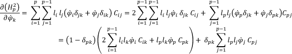
where δ is Kronecker delta. It's worth noting that it should be δ _jk = 0, (j = 1 …p - 1), if k = p.

Hence;

$\begin{array}{c}\frac{d}{dt}\left(\frac{\partial \left(H_p^2\right)}{\partial {\dot{\phi }}_k}\right)=\left(1-{\delta }_{pk}\right)\\ \left(2\sum _{i=1}^{p-1}{l}_i{l}_k\left({\ddot{\phi }}_i C_{ik}-{\dot{\phi }}_i\left({\dot{\phi }}_i-{\dot{\phi }}_k\right)S_{ik}\right)+l_p{l}_k\left({\ddot{\phi }}_p C_{pk}-{\dot{\phi }}_p\left({\dot{\phi }}_p-{\dot{\phi }}_k\right)S_{pk}\right)\right)\\ + {\delta }_{pk}\sum _{j=1}^{p-1}{l}_p{l}_j\left({\ddot{\phi }}_j C_{pj}-{\dot{\phi }}_j\left({\dot{\phi }}_p-{\dot{\phi }}_j\right)S_{pj}\right)\end{array}$

(A4)

Moreover;

$\begin{array}{c}\frac{\partial \left(H_p^2\right)}{\partial {\phi }_k}= \sum _{i=1}^p\sum _{j=1}^{p-1}{l}_i{l}_j{\dot{\phi }}_i{\dot{\phi }}_j \frac{\partial C_{ij}}{\partial {\phi }_k} =\sum _{i=1}^{p-1}\sum _{j=1}^{p-1}{l}_i{l}_j{\dot{\phi }}_i{\dot{\phi }}_j\left(-S_{ij}{\delta }_{ik}+S_{ij}{\delta }_{kj}\right)+ \\ \sum _{j=1}^{p-1}{l}_p{l}_j{\dot{\phi }}_p{\dot{\phi }}_j\left(-S_{pj}{\delta }_{pk}+S_{pj}{\delta }_{kj}\right)=\left(1-{\delta }_{pk}\right)\\ \left(2\sum _{i=1}^{p-1}{l}_i{l}_k{\dot{\phi }}_i{\dot{\phi }}_k S_{ik}+l_p{l}_k{\dot{\phi }}_p{\dot{\phi }}_k S_{pk}\right)-{\delta }_{pk}\sum _{j=1}^{p-1}{l}_p{l}_j{\dot{\phi }}_p{\dot{\phi }}_j S_{pj}\end{array}$

(A5)

By substituting the Eqs. A4 and A5 in following it's obtained:

$\begin{array}{c}\frac{d}{dt}\left(\frac{\partial T}{\partial {\dot{\phi }}_k}\right)-\mathrm{ }\frac{\partial T}{\partial {\phi }_k}=\mathrm{ }\sum _{p=1}^n{I}_p{\ddot{\phi }}_p{\delta }_{pk}+\frac{1}{2}\sum _{p=1}^n{m}_p\left(\frac{d}{dt}\left(\frac{\partial \left(H_p^2\right)}{\partial {\dot{\phi }}_k}\right)-\mathrm{ }\frac{\partial \left(H_p^2\right)}{\partial {\phi }_k}\right)=I_k{\ddot{\phi }}_k\\ +\frac{1}{2}\mathrm{ }\sum _{p=k}^n{m}_p\left(\left(1-{\delta }_{pk}\right)\left(2\sum _{i=1}^{p-1}{l}_i{l}_k\left({\ddot{\phi }}_i\mathrm{ }{C}_{ik}-{\dot{\phi }}_i^2{S}_{ik}\right)+l_p{l}_k\left({\ddot{\phi }}_p\mathrm{ }{C}_{pk}-{\dot{\phi }}_p^2{S}_{pk}\right)\right)+\mathrm{ }{\delta }_{pk}\sum _{j=1}^{p-1}{l}_p{l}_j\left({\ddot{\phi }}_j\mathrm{ }{C}_{pj}+{\dot{\phi }}_j^2{S}_{pj}\right)\right)\end{array}$

(A6)

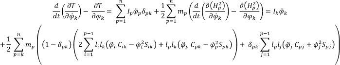
It can also be rewritten in an abbreviated manner as follows;

$\begin{array}{c}\frac{d}{dt}\left(\frac{\partial T}{\partial {\dot{\phi }}_k}\right)- \frac{\partial T}{\partial {\phi }_k} \equiv \mathrm{ }{I}_k{\ddot{\phi }}_k+\frac{1}{2} \sum _{p=k}^n{m}_p\left(\left(1-{\delta }_{pk}\right)\left(2\sum _{i=1}^{p-1}\mathrm{M}\left(i,k\right)+\mathrm{M}\left(p,k\right)\right)+ {\delta }_{pk}\sum _{j=1}^{p-1}\mathrm{M}\left(j,p\right)\right)\\ =I_k{\ddot{\phi }}_k+\frac{1}{2} \sum _{p=k+1}^n{m}_p\left(2\sum _{i=1}^{p-1}\mathrm{M}\left(i,k\right)+\mathrm{M}\left(p,k\right)\right)+ \frac{m_k}{2}\sum _{j=1}^{k-1}\mathrm{M}\left(j,k\right)\end{array}$

(A7)

where $\mathrm{M}\left(a,b\right)=\left(l_a{l}_b{\ddot{\phi }}_a{C}_{ab}-{\dot{\phi }}_a^2{S}_{ab}\right)$ . These should be also noted that: ${\delta }_{pk}{S}_{pj}=-{\delta }_{pk}{S}_{jp}=S_{jk}$ , and $\forall p<k:\frac{\partial \left(H_p^2\right)}{{\partial }_{qk}}=0$ , where q = φ, φ̇.

Furthermore, the total gravity potential energy is given as:

$V=\sum _{p=1}^n{m}_{p}g{\bar{h}}_p=g\sum _{p=1}^n{m}_p\left(\sum _{i=1}^p{l}_i\mathrm{s}\mathrm{i}\mathrm{n}{\phi }_i- \frac{l_p}{2} \mathrm{s}\mathrm{i}\mathrm{n}{\phi }_p\right)$

(A8)

Hence it is obtained that:

$\begin{array}{c}\frac{\partial V}{\partial {\phi }_k}=g\sum _{p=1}^n{m}_p\left(\sum _{i=1}^p{l}_i\mathrm{c}\mathrm{o}\mathrm{s}{\phi }_i{\delta }_{ik}- \frac{l_p}{2} \mathrm{c}\mathrm{o}\mathrm{s}{\phi }_p{\delta }_{pk}\right)=\\ g\left(\sum _{p=k}^n{m_{p}l}_k\mathrm{c}\mathrm{o}\mathrm{s}{\phi }_k- m_k\frac{l_k}{2} \mathrm{c}\mathrm{o}\mathrm{s}{\phi }_k\right)=\left( \frac{m_k}{2}+\sum _{p=k+1}^n{m}_p\right) g{ l}_k\mathrm{c}\mathrm{o}\mathrm{s}{\phi }_k\end{array}$

(A9)