
Abstract
This article is intended to present a multibody dynamic model of the drilling system, consisting of drillstring and drilling fluid. The drillstring is a complex rigid–flexible coupling system, including rigid bodies, Euler–Bernoulli beam elements, constraints and dynamic loads, and its dynamic model is established using the absolute nodal coordinate formulation. The drilling fluid, composed of internal, annulus, and under-bit fluids, is modeled as one-dimensional compressible fluid; the relative flow of the drilling fluid is modeled using the Arbitrary Lagrangian–Eulerian description; the force of the drillstring acting on the drilling fluid is introduced through the drilling fluid transport motion; meanwhile, the reaction force acting on the drillstring is taken as an external load. The contact between the drillstring and drilling fluid is simulated based on Hertz contact theory, and the rock penetration model is built based on the rock-breaking velocity equation. Based on this model, the coupled vibration of the drillstring and the effects of the drilling fluid flow rate and density on the drilling process are investigated through several examples.
Keywords
Introduction
In drilling engineering, due to the interaction of the drillstring with the drilling fluid, as well as the dynamic contact between the drillstring and the wellbore, the drilling system is a complex nonlinear fluid–solid coupling system. Therefore, it is necessary to establish a model with high computational accuracy and efficiency that can simulate the dynamic behavior of the drillstring sliding and rotating in the wellbore filled up with drilling fluid.
Several methods have been widely implemented to investigate the dynamic characteristics of the drillstring system, such as the finite element method (FEM),1–4 the differential equation method, 5 and other analytical solution.
Although these methods are relatively mature, there are still some deficiencies in practical applications due to the low computational efficiency or the over-simplification of the system. For example, the FEM has some difficulty in simulating the large deformation of the drillstring with large slenderness ratio and the dynamic contact between the drillstring and the wellbore. 6 Recently, the multibody dynamic method is developed to investigate the drilling system.7,8 In the typical model, the slender flexible drillstring is simulated with absolute nodal coordinate formulation (ANCF) 9 beam element. Meanwhile, the contact between the drillstring and the wellbore is modeled based on Hertz contact theory. 6 Compared with FEM, the multibody dynamic method can well simulate not only the three-dimensional rotation, large deformation, and large displacement of the drillstring but also the dynamic contact of the system. Furthermore, this method also has significant advantage in the calculation speed. 10
Since the slender drillstring is rotating and sliding in the wellbore filled up with drilling fluid, the interactions of the drillstring with the drilling fluid may have some influence on the dynamic behavior of the drilling system. Although there has been considerable studies in modeling and analyzing the dynamic characteristics of the system, such as the coupled vibration of the drillstring system,11,12 the study that takes into account the coupling of the drillstring and drilling fluid is still lacking,1,13 especially for investigating the effects of the drilling fluid on the drilling process.
In this article, a new simulation model of the drilling system considering the coupling of the drillstring and the drilling fluid is established using the multibody dynamic approach. In this model, the motion of the drilling fluid is described using the Arbitrary Lagrangian–Eulerian (ALE) method, 14 the drillstring is modeled as ANCF beam with several contact detection points, and then the contact between the drillstring and the wellbore is simulated based on Hertz contact theory. Furthermore, the rock penetration process has also been considered. Therefore, this model can be used to simulate the coupled vibration and the drilling process of the system with emphasis on the effects of drilling fluid.
The following context is organized in this way. Section “The dynamic model of the drilling system” establishes the dynamic equations of the drilling system using the multibody system dynamic approach. Then, the effects of the drilling fluid on the coupled vibration and the drilling process of the system are investigated in section “The effects of drilling fluid on the dynamic behavior of the drilling system.” Conclusions are given in section “Conclusion,” subsequently.
The dynamic model of the drilling system
The drilling system is a complex fluid–solid coupling dynamic system, as shown in Figure 1. The system has two subsystems: the drillstring and the drilling fluid. The drillstring subsystem consists of several rigid and flexible bodies with constraints between each other. And, the drilling fluid subsystem is composed of internal, annulus, and under-bit fluids. To establish the dynamic model of the drilling system, the dynamic equations of the drilling fluid and drillstring are derived, respectively.
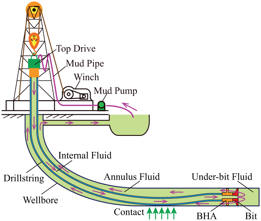
The schematic representation of the drilling system.
The dynamic equations of the drilling fluid
The relative flow of the drilling fluid is modeled based on framework of the ALE description. 14 The force of the drillstring acting on the drilling fluid is introduced through the drilling fluid transport motion, and the reaction force acting on the drillstring is taken as an external load.
To establish the dynamic equations of the drilling fluid, following assumptions are adopted:
The drilling fluid is a one-dimensional compressible flow.
Volumetric strain is proportional to the pressure and the increment area of the channel cross section is proportional to pressure.
The formula of pressure loss for steady flow is also available for the unsteady flow.
The axial stretch effect of the channel is considered.
There is no heat exchange in the subsystem.
The generalized coordinates and mass equation of the drilling fluid
Fluid flux

Thus

where
As shown in Figure 2, assuming that the channel length changed from initial length
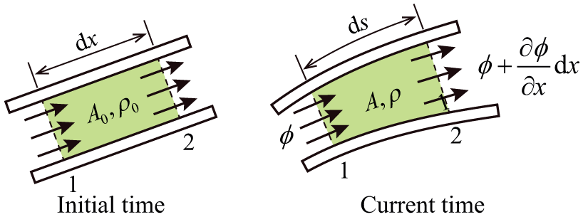
The schematic representation of the fluid mass conservation.
According to the mass conservation

And then
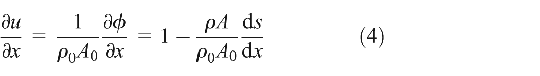
Equations (2) and (4) are the derivative expressions of u. Adopting the equivalent displacement to describe the motion of the fluid can automatically satisfy the mass equation, and therefore is convenient.
The momentum equations of the fluid and the reaction force acting on the string
Since the drilling fluid is composed of internal, annulus, and under-bit fluids, therefore, the momentum equations of these three kinds of fluids will be derived, respectively.
As shown in Figure 3, the mass center of the internal fluid always coincides with the section center of the drillstring

where

The schematic representation of the momentum balance of the internal fluid.
According to the derivation rule of material derivative, the velocity and acceleration of the internal fluid are expressed as

where
There are several forces acting on the internal fluid: the gravity, the pressure force of the end face, the pressure, and friction force caused by drillstring inter wall. They are expressed as follows:
Pressure force on section 1
Pressure force on section 2

Gravity

Pressure force on the drillstring inter wall

Friction force on the drillstring inter wall

where
According to Newton’s second law, the acceleration of internal fluid is balanced with external force

Three-dimensional dynamic equation of the internal fluid is obtained by simplifying equation (7), expressed as

where
Since
The additional pressure caused by the area change in channel can be ignored.
The one-dimensional dynamic equations of the internal fluid can be obtained by projecting equation (8) to the direct
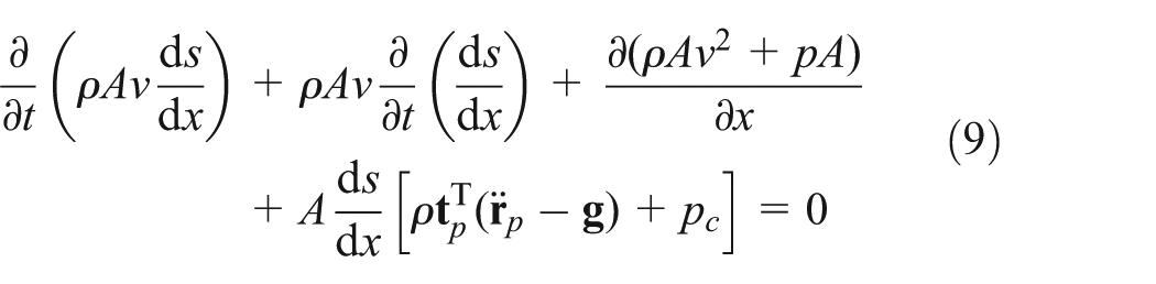
The first term represents the time rate of change of fluid momentum, the second term represents the additional inertia force caused by channel expansion, the third term represents the gradient of fluid hydrodynamic pressure, and the fourth term represents the external forces including relative motion, gravity, and friction. When the effect of channel expansion is not considered, equation (9) can be degenerated to classical one-dimensional flow equation

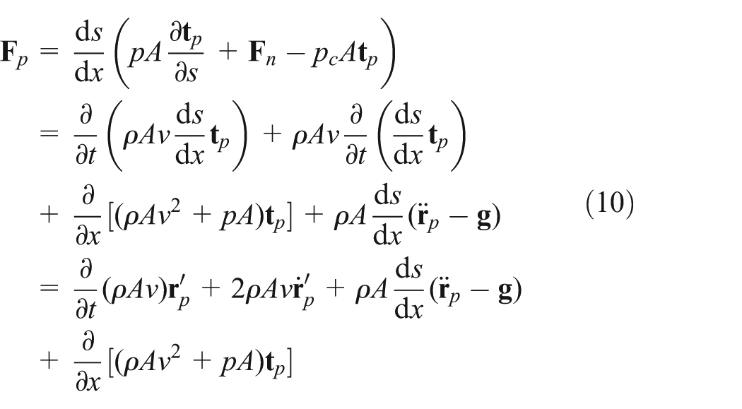
Considering that the pressure and friction forces by the drillstring inner wall is the reciprocal force between the drillstring and the drilling fluid, rejecting the two forces in equation (8), the remaining forces are the reaction forces of the internal fluid acting on the drillstring, expressed as
As shown in Figure 4, although the mass center of the annulus fluid not always coincides with the section centroid of drillstring, the projections of the two vectors along the borehole direction are equal. In addition, the static moment of wellbore cross section relative to coordinate system o-xyz equals to the sum of that of annulus fluid section and drillstring section. Then, the following relationship can be obtained

where

where


The schematic representation of the momentum balance of the annulus fluid.
As well as

According to the derivation rule of the material derivative, the velocity and acceleration of the annulus fluid are obtained as

where

is the flow transformation matrix of the annulus fluid,

Comparing equations (6) and (15), we find the transformation matrix
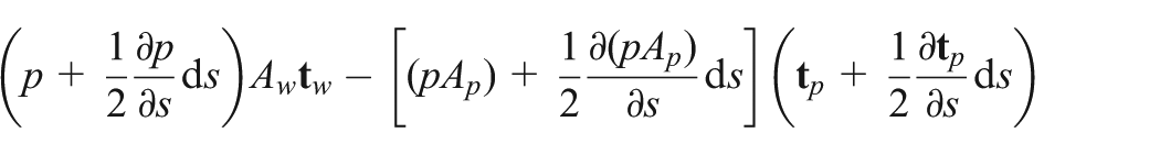
The forces acting on the annulus fluid are gravity, pressure force on the end face, pressure, and friction force caused by the drillstring outer wall and borehole inter wall. They are expressed as follows:
Pressure force on section 1
Pressure force on section 2
Gravity

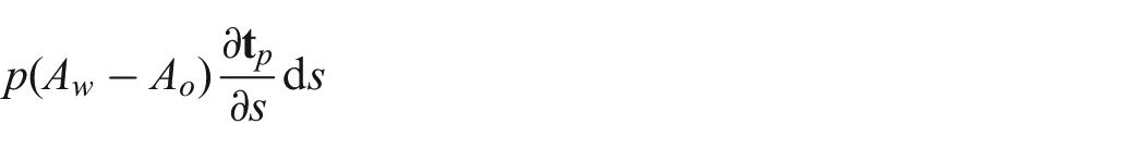
Pressure force on the outer wall of drillstring
Pressure force on the inter wall of borehole
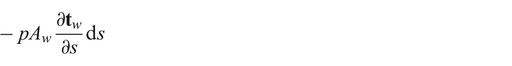
Friction force on the outer wall of drillstring

where
Friction force on the inter wall of borehole

where
The normal force acting on the fluid by drillstring is
According to Newton’s second law, the acceleration of annulus fluid is balanced with external force

Simplified

Combining the frictions caused by drillstring and the borehole, the three-dimensional dynamic equations of the annulus fluid are expressed as
where
Because

the additional pressure caused by the change of channel area can be ignored.
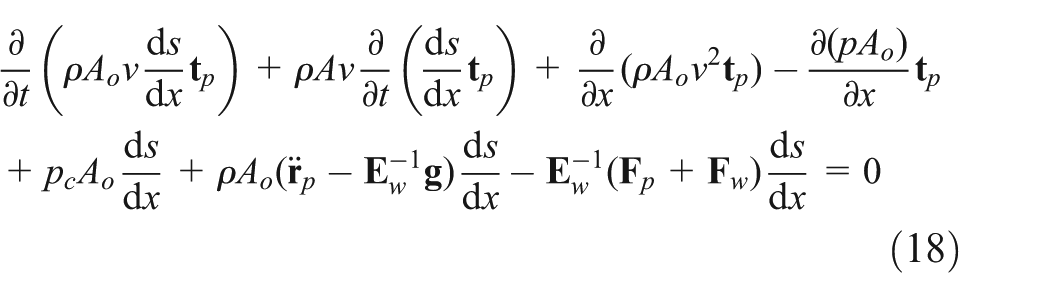
The one-dimensional dynamic equations of the annulus fluid are obtained by projecting equation (18) to the direct

In this equation, the first term represents the time rate of change of fluid momentum, the second term represents the additional force caused by channel expansion, the third term represents the gradient of fluid hydrodynamic pressure, and the fourth term represents the external forces including relative motion, gravity, and friction. When the effect of channel expansion is not considered, equation (19) can also be degenerated to classical one-dimensional flow equation

Investigating the one-dimensional flow equations of the internal fluid and the annulus fluid, we find the main difference is that the internal fluid is projecting to
Altogether, the pressure and friction force on the drillstring outer is the reciprocal forces between the drillstring and the fluid, the same as the reciprocal forces between the borehole and fluid. By rejecting the interaction forces mentioned above in equation (19), the remaining forces are the reaction forces by the annulus fluid acting on the drillstring, expressed as

where
The momentum equations of the under-bit fluid can be obtained by replacing
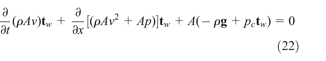
The one-dimensional dynamic equations are obtained by projecting equation (22) to

Obviously, there is no reaction force acting on the drillstring caused by under-bit fluid.
The constitutive equation of the drilling fluid
The constitutive equation of one-dimensional compressible fluid is

where E is the equivalent elastic modulus of drilling fluid,
Integrating equation (24) once and according to equation (4), the following equation can be obtained

Furthermore, the expansion of the channel area can be expressed as

Considering that

the additional pressure caused by the elastic transmutation of the channel area is so small that it is neglected. Therefore, a simplified constitutive equation is used

where the equivalent elastic modulus E is coalescence of the fluid compression coefficient
The fluid compression coefficient is related to the fluid type, temperature, and pressure. However, the change of
The channel elasticity coefficient can be easily derived based on the elastic theory, the elasticity coefficient of internal flow channel is

The elasticity coefficient of the annulus flow channel is

where
Flow pressure loss of the fluid
There is flow resistance term in the dynamic equation of the drilling fluid, and the resistance, presented as flow pressure loss, is mainly caused by on-way resistance and related with the viscosity property, the state, and the rheological model of the drilling fluid. In drilling engineering, the drilling fluid viscosity is measured by direct-indicating viscometer. The rheological properties of the drilling fluid are complex. The most widely used models are power law, Bingham, Casson, and Herschel–Bulkley (HB). In this article, the power law model assumed that the fluid shear stress

where K is the consistency index, and n is the flow behavior index. They can be obtained as 15

where
Then, the pressure loss of the internal fluid can be expressed as

where

And, the pressure loss of the annulus fluid can be obtained as

where

In the equations above,

where
The dynamic equations of the drilling fluid
By coupling the equation of momentum and constitutive equation, the dynamic equations of the drilling fluid are obtained as
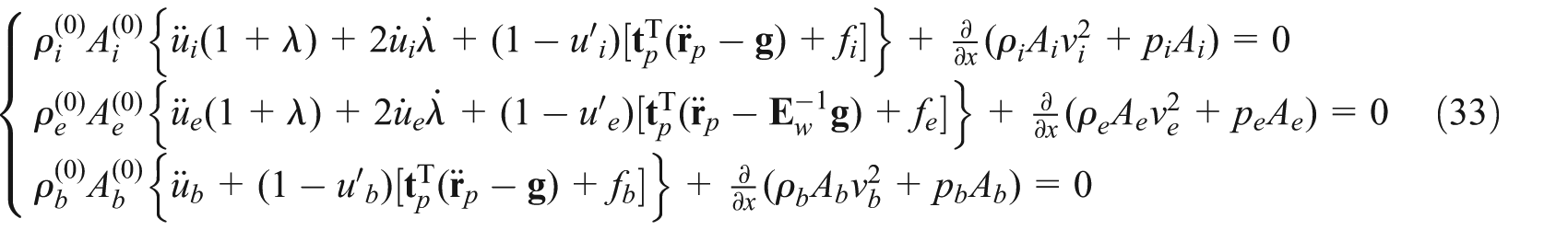
and the reaction force acting on the drillstring is

In the above equations, the subscripts i, e, and b represent internal, annulus, and under-bit fluids, respectively.
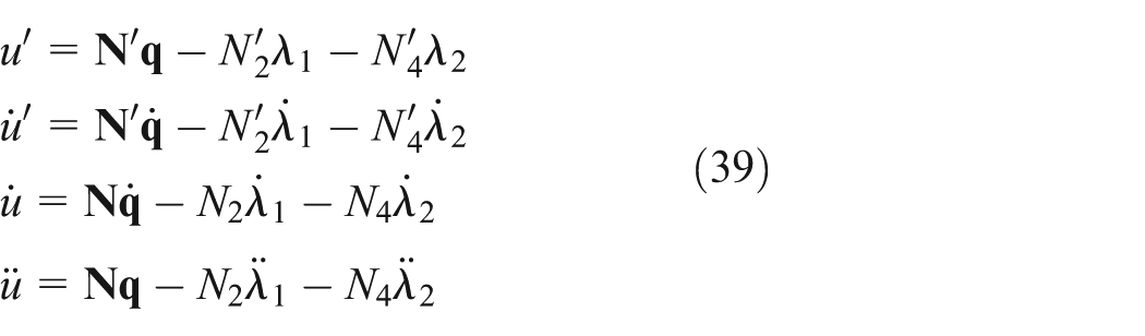
Dividing the channel into several segments and creating fluid node at the section, the neighboring two nodes construct one element. The equivalent displacement u and fluid strain

The equivalent displacement gradient of the element can be obtained at the nodes

Hermite interpolation is applied to describe the equivalent displacement of the element

where

By substituting equation (36) into equation (37), the interpolation formula using generalized coordinates can be obtained as

where

is the interpolation function matrix of the element. Furthermore, the partial derivatives of the generalized gradient are obtained as
where

is the gradient matrix of element interpolation function.
Using Galerkin integration method and adopting the shape function as the weight function, the element integral equations of the internal fluid can be obtained as
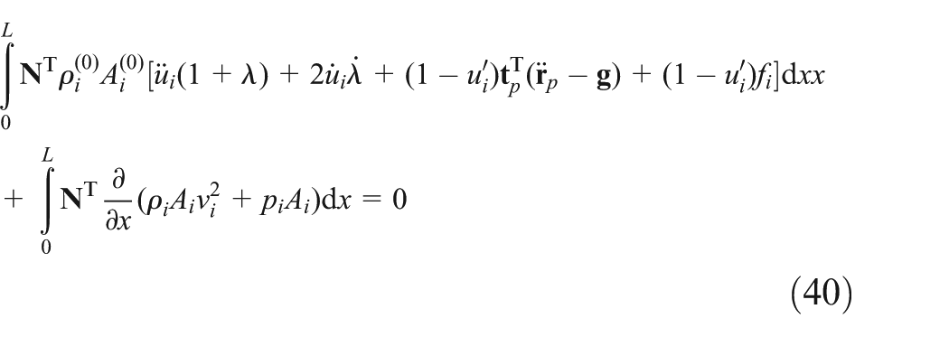
The weak solution of equation (40) can be obtained by integrating the second term using partial integration once

In the equations above, u is the only requested one-order continuous that satisfies the property of Hermite interpolation

Equation (42) represents the integral boundary of the pressure and has three cases:
Middle node. Integral boundary term is counteracted by the neighborhood elements.
Displacement boundary node. Integral boundary term is replaced by the constrained force.
Force boundary node. Boundary term is applied using force.
So, when the dynamic equations of all the fluid elements are assembled, the boundary term (42) would not be retained.
Finally, the finite element equation of the drilling internal fluid can be expressed as
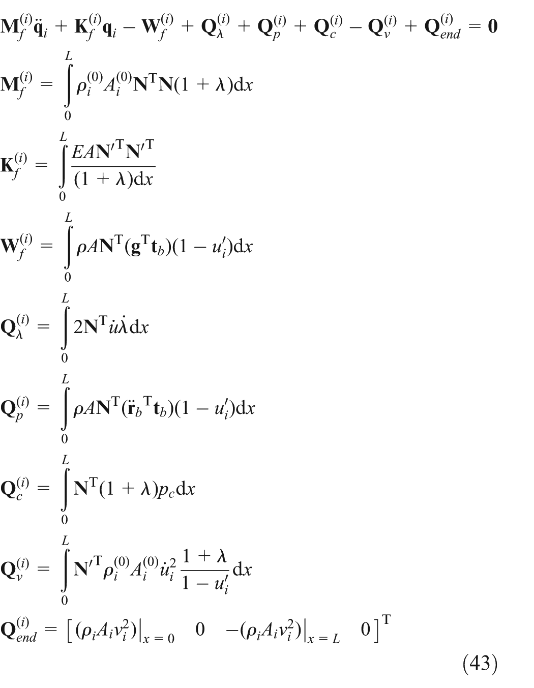
where
Similarly, the finite element equations of the annulus and under-bit fluids can be obtained using weighted residual method

And the reaction forces of the drilling fluid acting on drillstring can be expressed as
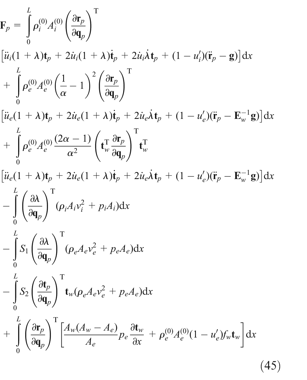
where

The dynamic equations of the drillstring system
The drillstring is modeled as a complex rigid–flexible coupling system which consists of rigid bodies, flexible beam elements, constraints, and dynamic loads. The dynamic equations of rigid body and flexible beam are divided, respectively.
Dynamic equations of rigid bodies
The top drive, the stabilizer, and the bit are modeled as rigid bodies in this article. The generalized coordinate

Based on the Lagrange equation, the dynamic equation of the rigid body can be expressed as 16

where

Dynamic equations of ANCF beam
The ANCF beam elements which can describe the motion, rotation, and deformation of the drillstring are used to model the flexible components of the drillstring. Although the theory of the ANCF beam has been proposed by Zhao and Ren, 17 it is preferred to introduce this element briefly for the integrity of this article.
A two-node beam element with cross-sectional area A and initial length L is shown in Figure 5, and the generalized coordinates of the nodes I and II are

where

The schematic representation of ANCF beam element.
Then, the generalized elemental coordinate is

Assuming that the arc-length coordinate of an arbitrary point on the axis of the beam element is x, then the isoparametric coordinate

According to the definition of normal strain, the derivatives of the centerline at nodes are

where

where

To describe the rotation of the beam element, the material reference frame

The symbol “′” denotes the derivative with respect to

where

Obviously, the final

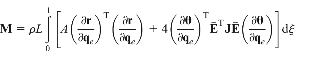
Then, the kinetic energy of the element is

where

The elastic potential work is

where E and G are the elastic and shear moduli, respectively, and
Therefore, the governing equations of the beam can be obtained by the Lagrange equation

where
Boundary conditions
Rock penetration equation
A three-dimensional rate of penetration (ROP) equation that considering the cutting bit anisotropy and the formation anisotropy is adopted to describe the rock penetration process.
By defining the coordinate system
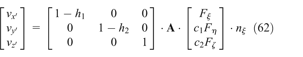
where
In the drilling simulation, the moving-down velocity and the rotary speed of the top drive are the main input parameters, while the bit weight and the actual drilling speed are the output parameters induced by the dynamic model. In order to determine the bit weight and the drilling speed, the forces acting on the bit by the wellbore should be calculated first. Therefore, the Hertz contact theory is adopted to model the interaction between the bit and the wellbore like an ellipsoid sphere in a bucket. Then, the bit weight could be easily counted. Furthermore, the drilling speed could be accomplished with equation (62), in which the other parameters are determined by the characterization of the stratum. It should be emphasized that the growth of the wellbore is implemented at the end of each integral step using the drilling speed multiplied with the step size which is along the direction of the bit axis.
Contact
The wellbore is modeled as a rigid hole with circular cross section, and a set of wellbore node is placed on the curved well centerline to describe the well trajectory, each wellbore node has nine parameters: the material coordinate, the position vector, the tangent direction, the radius, and the sliding friction coefficient. In petroleum engineering, the well trajectory is described with the measure depth (the arc length of the well trajectory from the start point of the well to the wellbore node), the inclination (the angle between the local tangent direction of the wellbore node with the vertical direction), and the azimuth (the angle between the projection of the trajectory on the horizontal plane with the north direction). And the parameters of the wellbore node can be transformed from the measure depth, the inclination, and the azimuth using the cubic Hermite interpolation. 6
Several detecting points are set on the axial line of the beam element. Therefore, the detection between the drillstring and the wellbore is transformed to the detection between detecting points and rigid cylinder, as shown in Figure 6.

The contact model between drillstring and wellbore.
According to the Hertz contact theory, the contact force

where
The support force

where k is the contact stiffness, e is the contact recovery index, and c is the contact damping.
The magnitude of friction force can be obtained by Coulomb model

where
Finally, the contact force is exerted on the nodes of the beam element. According to the virtual work principle, the generalized contact force acting on the element can be expressed as

where
The dynamic equations of the drilling system
The string is divided into several segments, each segment is one element, and the two ends of the segment are selected as the node, then the dynamic simulation model of the string can be established. The nodes of internal and annulus fluids are appended to the string nodes that have the same location. The dynamic equations of the whole system can be obtained by assembling equations (44), (48), and (61). Using the multibody dynamic system method, these three equations can be expressed as

where equation (a) is the dynamic equation of the system, equation (b) is the holonomic constraint equation of the system, and equation (c) is the non-holonomic constraint equation;
The equations of the system form a set of differential algebraic equations (DAEs), which can be solved by the implicit first-order backward differentiation formula (BDF) method. 6
Effects of drilling fluid on the dynamic behavior of the drilling system
Coupled vibration of the drillstring
Due to the contact of the drillstring with the wellbore, the contact of the bit and formation, as well as the unbalance mass and the initial curvature of the drillstring, the coupled vibration will occur when the drillstring rotates in the wellbore. Typical forms are axial, torsional, and lateral vibrations. A coupling model of drilling system with a constant top drive rotary speed is established to investigate the influence of the drilling fluid on the coupled vibration.
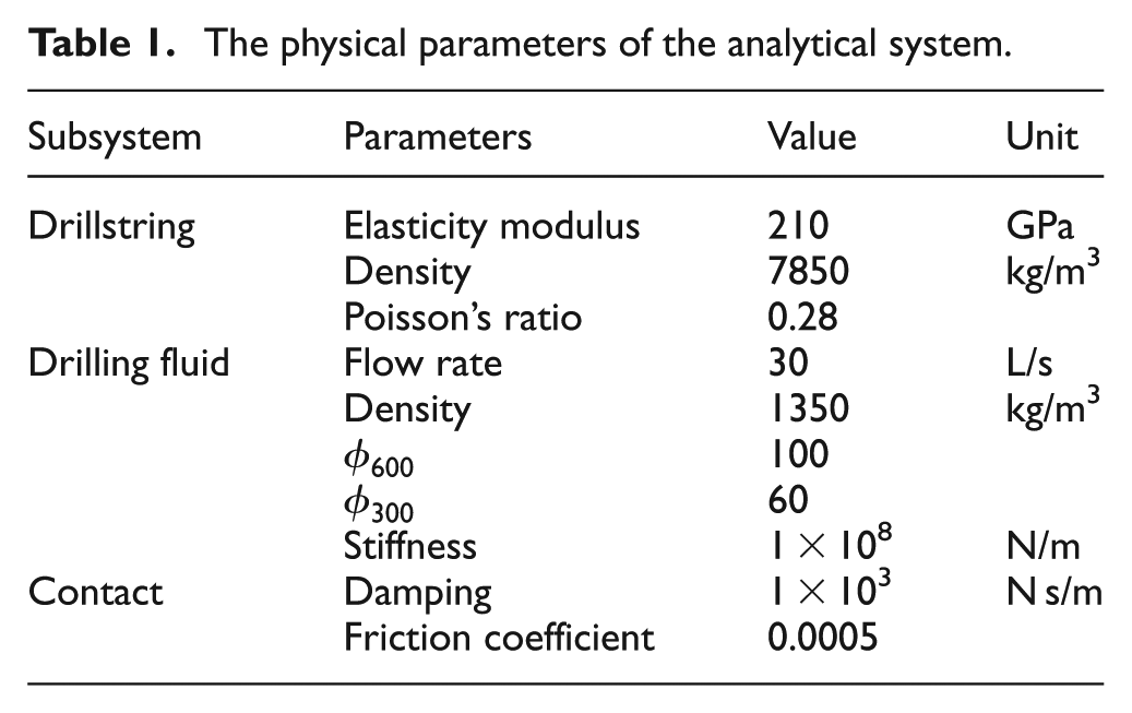
Without loss of generality, the wellbore is assumed to be vertical and its measure depth is 2000 m, the dimension of the drillstring is shown in Figure 7, where “OD” and “ID” denote the outside and inside diameter, and the physical parameters of the drillstring and drilling fluid are shown in Table 1. The rotary speed of the top drive is 80 r/min. Through the mesh convergence test, the drillstring is discretized into 225 elements. And, the element number of internal and annulus fluids is equal to drillstring.

The schematic representation of the analytical system.
The physical parameters of the analytical system.
For the convenience of discussion, another simulation model without drilling fluid, named as “drillstring model,” is established for comparison.
The axial vibration
The axial vibration can be characterized by the fluctuation of the bit pressure. The bit pressures of the two models are shown in Figure 8. It can be found that the fluctuation of the bit pressure approximates periodic fluctuation, and the difference of the two models is not obvious.
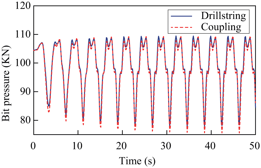
The bit pressure of the two models.
The torsional vibration
The torsional vibration is usually caused by the friction between the drillstring and the wellbore. When the driver rotates at constant speed, the bit speed is 0–2 times that of top driver. As shown in Figure 9, the bit speed curves of the two models are almost consistent.

The speed of the bit.
The whirling motion
The typical transverse vibration is the whirling motion. The unbalance mass or other interference force may cause the string revolve around the borehole axis and rotate on its axis.
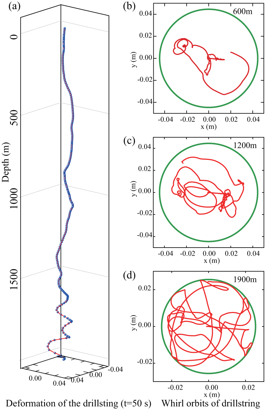
Figures 10(a) and 11(a) show the deformation of the drillstring at the end of the simulation, and Figures 10(b)–(d) and 11(b)–(d) are the center whirl orbits of drillstring at measure depths 600, 1200, and 1900 m.

Whirling motion of the coupling model (a) Deformation of the drillsting (t = 50 s). (b–d) Whirl orbits of drillstring.
Whirling motion of the drillstring model (a) Deformation of the drillsting (t = 50 s). (b–d) Whirl orbits of drillstring.
Due to the lower drillstring subjected to compression, the whirling motion occurs more easily compared with the upper drillstring, as shown in Figure 10. According to the dynamic response of the system, we found that the whirling motion of the coupling model is more likely to occur at the constant rotary speed and the drillstring deformation is larger. In contrast, the drillstring remains in the center of the borehole when the effect of drilling fluid is ignored. Of particular note is that the helical deformation appeared in the collar of the coupling model and the collar outward against the borehole well.
In short, the drilling fluid has little influence on the axial and torsional vibration of the drillstring but leads to the whirling motion is easier to occur, and this influence needs more research in the future.
Effects of drilling fluid on the drilling process
Several simulation models with different drilling fluid parameters are established to investigate the effects of the flow rate
The well trajectory and the inclination angle of the system with different parameters are shown in Figures 12 and 13. In the following section, the effects of the flow rate and density of the drilling fluid will be discussed, respectively.
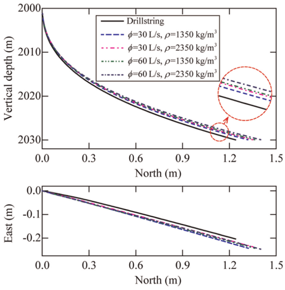
The well trajectory of the system with different drilling fluid parameters.

The inclination angle of the system with different drilling fluid parameters.
Comparing the well trajectory and inclination angle of the simulation model with different flow rates with that of the simulation model without drilling fluid, it is found that the well trajectory of the system with low flow rate is close to the system without drilling fluid. As the flow rate increases, the difference becomes greater.
On the other hand, the inclination angle increases with the increase in the density of the drilling fluid, especially when the flow velocity increases at the same time.
For a further discussion, the effect of the drilling fluid on the drilling process and the concept of average buildup rate are used. Assuming that the new well trajectory approximates to a circle arc, then the average buildup rate is defined as

where
The average buildup rate of the simulation models.

It is found that the average buildup rate of the system increases with the increase in flow rate and density of the drilling fluid. But viewed as a whole, the influence of flow rate is more significantly than the density.
The difference of average buildup between the model with
Conclusion
A fluid–solid coupling model of the drilling system based on the multibody dynamic system method is proposed for simulating the dynamic behavior of the drilling system with emphasis on the effects of drilling fluid. In this model, the relative flow of the drilling fluid is modeled using ALE description, and the dynamic equation of the slender flexible drillstring is established by the ANCF. Meanwhile, the model takes into account the contact between the drillstring and the wellbore as well as the rock penetration process, so this model can be used to simulate the coupled vibration and drilling process.
The effects of the drilling fluid on the dynamic behavior of the system are investigated. The simulation results show that the drilling fluid has significant influence on the whirling motion of the drillstring: the whirling motion will appear easily when the drillstring rotates in the wellbore filled with drilling fluid. Furthermore, the contact between the drillstring and wellbore is frequent and continuous. The deflecting capacity of the system increases with the increase in flow rate and the density of the drilling fluid. For the drilling system with high flow rate, the influence of the drilling fluid on the drilling process should be considered.
The simulation examples show that the proposed model is capable of describing the dynamic behavior of the drilling system and provides a potential accurate and efficient simulation model in drilling engineering.
Footnotes
Academic Editor: Chuanzeng Zhang
Declaration of conflicting interests
The author(s) declared no potential conflicts of interest with respect to the research, authorship, and/or publication of this article.
Funding
The author(s) disclosed receipt of the following financial support for the research, authorship, and/or publication of this article: This work was supported by the Open Fund Project of the State Key Laboratory of Offshore Oil Exploitation (Grant No. 2013-YXZHKY-020).