Sage Journals: Discover world-class research

Abstract

The purpose of this paper is to propose a systematic smooth control method for improving the stability of the two-wheeled self-balance robot under impact disturbances. For enhancing the robtot stability, a blend controller based on states feedback control embedded with the PID speed synchronization is estabilished, as well as a hybrid filter composes of RC network and Kalman algorithm. With the hybrid filter, disturbance signals are maximally attenuated or directly eliminated, and the system sensitivity to the impact disturbances significantly declines; under the blend motion controller, the robot can not only keep balance under impacts but also achieve synchronization of the two driving wheels. The dynamic model, the blend controller, hybrid filter, and experimental results including application to transport are described, both of the simulation and experimental results are provided to verify the analysis.

Keywords

Smooth control two-wheeled robot compact disturbances

1. Introduction

Two-wheeled coaxial robots, with their outstanding advantages, such as compact in mechanical structure, flexibility in motion and portability, have attracted considerable attentions in the past decades, JOE (Grasser, D'Arrigo et al. 2002), nBOT(Anderson. 2007) and many other similar robots have been reported over worldwide. Balance control is one of the research issues, and a variety of control methods have been proposed for it, such as sliding model (Rong-Jong and Li-Jung 2006; Huang, Guan et al. 2010), adaptive control(Rong-Jong and Li-Jung 2006) and state feedback(Shiroma, Matsumoto et al. 1996; Grasser, D'Arrigo et al. 2002; Pathak, Franch et al. 2005). Although balance control is fundamental for the self-balance robots, it is not the ultimate research goal. For a robot with practical values, balance control is the basis, and it needs to have good stability no matter disturbed or not, especially under the impact disturbances. Otherwise, a tiny impact disturbance may be a fatal unstable resource, and even directly cause the robot out of balance. When used as a mobile robot platform, instability caused by the impact may lead to damages of the airborne equipment; and conditions may even worse when it is as a personal transport, for serious security problems may happen when it suddenly lose its balance. Therefore, studying how to decay the impacts and realize stability is meaningful and important. In spite of many studies have been published concerning the balance control, but few attentions are paid to the impact disturbance. In reference (Zhou, Wu et al. 2004), the authors build a disturbance observer for controlling the robot and give the simulation results, it shows that the system has better ability to restrain disturbances and improved motion capabilities. It is obviously that interference studies can improve system stability. Different from with the former researches, we focus on a new systematic way to attenuate the impact disturbances, which is easier to implement.

In the balance control studies, states feedback control may be the most popular and successful one so far. Different types of states feedback control method are used to control the robot balance (Gans and Hutchinson 2006; Butler and Bright 2008). However, the robot speed not the wheel speed is selected as the state variables in the modelling process. So for the robot speed, it is a close control loop, but for the two driving wheels, it is open-loop. Speed of the two driving wheels may different and can not realize a line running. As a result, it is necessary to add a close-loop in order to get smooth control, whether in equilibrium or in the running condition. PID (proportion, integrated and differential) control with its outstanding performance has successful applications in the past researches. Consequently, we propose to add a PID sub-controller to the states feedback controller to achieve double-loop controller in this paper.

At the same time, no matter what kind of control method is used, accurate estimates of system state information is a fundamental problem. For instance, the simple way of estimating the absolute angle of the robot is to integrate the angular velocity out from a gyro. However, it will be inadequate over prolonged periods of time, because drift in the gyro signal will result in a ramping error in the position measurement. This problem is described in reference (Ashokaraj, Silson et al. 2002; Chen 2003; Imamura, Takei et al. 2008), and the authors had to design a special compensator to deal with. In this paper, we get the tilt angle from direct measurement rather than integration; an accelerometer and a gyro compose the measurement system, the accelerometer measures the robot tilt angle, and the angular velocity is measured by the gyroscope. In this way, the accelerometer provides a good low-frequencies estimate of its orientation in gravity, and it can get a better response in the effective frequency range of the robot. A gyro measures only the absolute angular rate. Although it can estimate the states value more accurate, a strong filter is more necessary. A hybrid filter based on RC network and Kalman filter for sensor signals filtering is designed. Unlike previous studies (Chen 2003; Imamura, Takei et al. 2008), the estimation method for the states values we proposed is compactable and highly effective, and it dose not need to consider the drift of the sensors.

This paper presents a control method to eliminate the impact of interference, so as to realize smooth control for the two-wheeled coaxial self-balance robot under the impact disturbances. The controller design, the blend filter and experimental results are also presented.

2. Controller design

The coaxial two-wheeled robot is inherent unstable and underactuated system (Andary, Chemori et al. 2008), all of the positions such as keep balance and running are realized by the torque of the two driving wheels, shown in Fig. 6. Theoretically, when the two driving wheels are fed by the same torque, the robot will only move in one direction (with a small forward and backward movement before the settlement is achieved)(Ahmad, Tokbi et al. 2009). Here, we only focus on the x direction and assume that the torques fed on the two wheels are the same. Fig. 1 shows the diagram of force acting on the robot, where the variables are defined as follows (McGill & King, 1995; Ren, Chen, Tsai, & Yao, 2004):

Figure 1.

Straight running model for the robot

m : Weight of one driving wheel

M : Weight of robot body

J_ω : Moment of inertia of the driving wheel

J_p : Moment of inertia of the robot body

R : Radius of the wheel

D : Distance between the two wheels

L : Distance from system Center of gravity to rotary axis

θ : Tilt angular of robot body

ω : Tilt angular speed of the robot body

x_m: Displacement of x direction

T_r, T_l: Torques of the driving wheels

Analysis system and operation of the forces, the following kinetics equations are established based on Newton analysis:

(T_{r} + T_{l}) / R = {\ddot{x}}_{m} (M + 2 m + 2 J_{ω} / R^{2}) + (\ddot{θ} \cdot \cos θ - {\dot{θ}}^{2} \cdot \sin θ) M L

(1)

\begin{array}{l} \ddot{θ} \cdot J_{P} = M (g - L \cdot \ddot{θ} \sin θ - L \cdot {\dot{θ}}^{2} \cos θ) L \cdot \sin θ - \\ - [{\ddot{x}}_{m} \cdot M + (\ddot{θ} \cdot \cos θ - {\dot{θ}}^{2} \cdot \sin θ) M \cdot L] L \cdot \cos θ - (T_{r} + T_{l}) \end{array}

(2)

For DC gear brush motors, following relationship exists, as shown in Equation (3):

T = - \frac{K_{m} K_{e} N^{2} ω_{m}}{R_{a}} + \frac{N K_{m} U}{R_{a}}

(3)

Where K_m, K_e is the motor constant, N is the reduction ratio, ω_m is the motor rotation angular speed, R_a is the motor resistance, T is the output torque of the reducer and U is the motor armature voltage.

Modifying (1) to (3) and then linearizing the result round the operating point (θ = 0, v = 0) the system's state space equations can be written in matrix form as:

[\begin{matrix} \dot{v} \\ \dot{θ} \\ \ddot{θ} \end{matrix}] = [\begin{matrix} 1 & 0 & 0 \\ a_{22} & a_{23} & 1 \\ a 42 & a_{43} & 0 \end{matrix}] [\begin{matrix} v \\ θ \\ \dot{θ} \end{matrix}] + [\begin{matrix} b_{21} & b_{21} \\ 0 & 0 \\ b_{41} & b_{41} \end{matrix}] [\begin{matrix} U_{l} \\ U_{r} \end{matrix}]

(4)

Where a₂₂, a₂₃, a₄₂, a₄₃, b₂₁, b₄₁ are constants determined by the system, and U_l, U_l are the armature voltage of the two motors.

A states feedback controller can be established according to Equation (4), and it only can achieve balance control and line running. In this controller, the robot velocity v is selected as the system state variable, and it is defined by Equation (5).

v = 0.5 (v_{l} + v_{r})

(5)

Where v_l and v_r are the speeds of the two driving wheels. From Equation (4), a close- loop is easy to establish for v, but for the speed of the two wheels, it is open-loop. This will lead to different speed of the two wheels, it is intolerable when the robot running in the line model for the existing of hunting. As a result, it is necessary to add a new loop after the state feedback controller to control the speed of the two wheels, and a PID controller maybe the best choice. Taking into account the amount of state space control of the controller is the armature voltage, we select the armature voltage is the output of the PID controller. The PID controller is easy to implement, and the controller we designed shown as follows:

u {(t)}_{lp} = K_{lP} e (t) + k_{li} \int e (t) dt + k_{ld} \frac{de (t)}{dt}

(6)

u {(t)}_{rp} = K_{rP} e (t) + k_{ri} \int e (t) dt + k_{rd} \frac{de (t)}{dt}

(7)

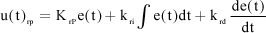
Where u(t)_*p is the output of the PID controller, and K_*P, k_*i, k_*d are the coefficients of the controller. The upper two equations are continuous. For the computer control, they can be deformed to discrete equations as:

u {(n)}_{lp} = K_{lP} e (n) + K_{li} \sum_{i = 0}^{n} e (i) + K_{ld} [e (n) - e (n - 1)]

(8)

u {(n)}_{rp} = K_{rP} e (n) + K_{ri} \sum_{i = 0}^{n} e (i) + K_{rd} [e (n) - e (n - 1)]

(9)

In this way, the structure of the equations becomes clear, where u(n)_*p is the motor control voltage in the control cycle n, e(n) is the velocity error, K_*P, K_*i and K_*d respectively are the proportional, integral and differential constants. In the actual designing of the controller, in order to make the algorithm compact and easy to implement, the right wheel speed is selected as the reference rate, and control the left wheel speed to follow with the right. Consequently, Equation (9) can be changed as:

u {(n)}_{rp} = u {(n)}_{reference} = k_{1} \cdot θ + k_{2} \cdot ω + k_{3} \cdot v

(10)

The left control voltage is:

u {(n)}_{lp} = k_{1} \cdot θ + k_{2} \cdot ω + k_{3} \cdot v + Δ u (n - 1)

(11)

Where Δu(n-1) = u(n)_lp - u(n)_reference.

Figure 2.

Hybrid controller

So far, a hybrid controller with two closed-loops has been established, the controller's inputs are the control voltages of the motors and outputs are the state variables. Although nominally there are two inputs, but from the Equation (5) can be seen walking in the completely line model, exactly the same input, can be considered a single-input system. Different from [4] [5], a PID closed-loop is added, so the new controller can control the robot in a state of equilibrium while to synchronize the speed of the two walking wheels at the same time.

3. Sensor basic relations

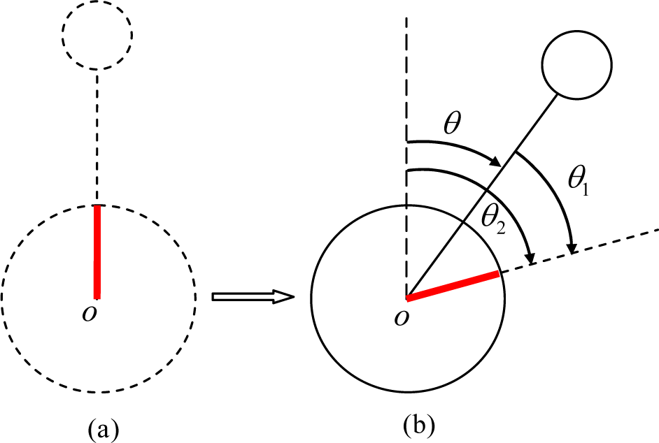
In the controller design process, v, θ and ω have been identified as system state variables. This sensor system determining the system state variables must be able to provide all the information, which determines the system-sensor system must be able to provide information for all state variables. We can get the absolute tilt angle θ of the robot body from the accelerometer, and we can also obtain the real-time angular velocity information of ω the gyro outputs. But we can not directly obtain the robot velocity v by Rotary encoders. A rotary encoder can only provide a relative measure of the rotation between two bodies. For the coaxial self-stabilizing robot, an encoder which measures the relative angle between the body and the wheel. For inverted coaxial self-stabilizing robot, to obtain the robot velocity v, it is necessary to combine the absolute tilt angle θ with the relative angle respect to the body, which is obtained from the rotary encoders, as shown in Fig. 3. In Fig. 3 (a), the robot is in a vertical state, all angles are zero; then the wheel runs a certain angle, as shown in Fig. 3 (b), it is clear that the angle θ₂ of the wheel turns and the absolute tilt angle θ of it has the following relationship:

θ_{2} = θ + θ_{1}

(12)

{\dot{θ}}_{2} = \dot{θ} + {\dot{θ}}_{1}

(13)

Where θ¹ is the relative angle of the robot with the wheel, and it could be directly obtained from the incremental encoder. As θ₂ is the absolute angle in respect to the gravity, so the robot's absolute speed v can be got by differential. To be clear, the above équations are vector rather than scalar.

Figure 3.

Relationships between the angles

4. Blend filter

4.1. RC networks for low pass filter

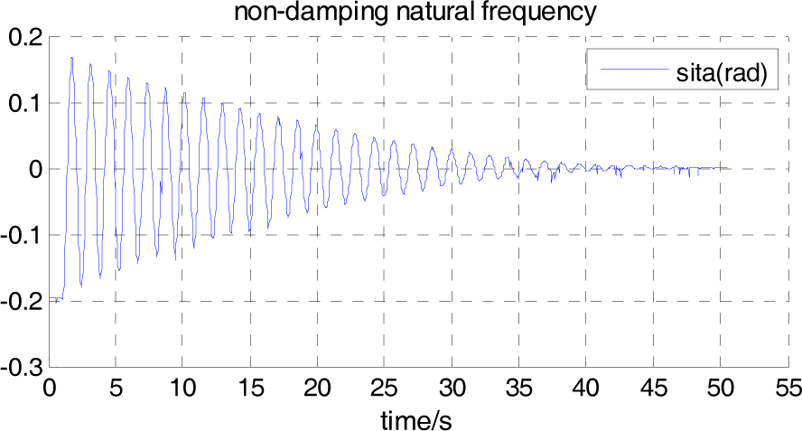
Obtains the undamped angular natural frequency of the robot by calculating is very difficult, but obtains it through test will be easy, as shown in Fig. 4, inverted to place the robot, while holding the wheels fixed. Pull the turning bar away from the equilibrium position and then let it go, recording all the data from swing to its stop in the balance position. Import the data to MATLB then get the testing drawing, as shown in Fig. 5, the natural period of oscillation t is about 1.45s. So it is convenient to calculate the natural angular frequency without damping of the robot is approximate 4.33rad/s. This angular frequency directly determines the designed filter cutoff frequency.

For the coaxial two-wheeled robot, it works in the low frequency range in most cases, high frequency signals will cause vibrations and make the robot lose balance, so a low pass filter is necessary. A first-order RC network is simple, low cost, and easy to implement. More importantly, it has very good low frequency performance, which the gain is constant 1 and the delay phase angle is too small to compensate. For our sensor system, using only a few resistors and capacitors will be able to form a low-pass filter unit with good effects, and it is applicable to any type of voltage output sensors.

For RC networks, there are two equations in our design are particularly important, as follows:

ω_{c} = 1 / τ

(14)

τ = RC

(15)

The cut-off frequency is determined Equation (14). For our filter, it is 9 rad/s for the gyro and 6.5rad/s for the accelerator.

Figure 4.

Testing the natural frequency

Figure 5.

Oscillation of the robot

4.2. Kalman filter for impact filter

Filtering effect of the RC network low pass filter unit is clear, there is an obvious reduction in the sensor signals burr and the signal stationary has been greatly improved, which can be verified from the model testing in the next section. Nevertheless, the sensor signals there are still needed to filter out the fluctuations in value. For instance, with the robot resting on the floor, the accelerometer output is a combination of rood vibrations and noise, some of the vibration values can not be filtered out with a RC network, which needs to adopt digital filter method, through the AD collection of digital data after digital filtering. In all of the digital filter algorithms, the Kalman filter has extensive and successful application (Ashokaraj, Silson et al. 2002). The Kalman filter (Widjaja, Shee et al. 2008) can be succinctly described as an optimal recursive data processing algorithm for systems corrupted by noise. It does not have to save all the data collected, only needs a previous state data for calculating, and can achieve high-speed recursive calculation, which is significant importance to the inherent unstable robot in terms of high real-time requirements. As a result, we choose the Kalman filter to deal with the digital fluctuations, to estimate the optimal values of the sensor data, the Kalman filter core are calculated as follows:

x (k | k - 1) = x (k - 1 | k - 1)

(16)

p (k | k - 1) = p (k - 1 | k - 1) + q

(17)

kg (k) = p (k | k - 1) / (p (k | k - 1) + r)

(18)

x (k | k) = x (k | k - 1) + k g (k) (z (k) - x (k | k - 1))

(19)

p (k | k) = (1 - kg (k)) p (k | k - 1)

(20)

The above equations are based on the following conditions: the system parameters A, B and H are 1, and there is none control variable U; q and r respectively are process noise and measurement noise covariance, and assume that their values are constant during the filtering process.

In all of the five equations, (16) and (17) are the estimated equations, (18) (19) and (20) are the recursive formulas. Note that the initial state value and covariance have to been set up before it starts to work.

5. Experiment and discussion

Experimental platform we use in the testing is a coaxial two-wheeled self-stabilizing robot, as shown in Fig. 6. It has a steer bar upon the body and two coaxial symmetrical arranged driving wheels. The system structure is simple and compact; it can work in the remote mode, autonomous mode or operation mode, using as a robot platform or a personal transporter with a maxim load of 70kg despite it's only about 20kg weight. A TA-25 accelerometer is used for the tilt angle measurement and a TFG-160D gyro is used to get the angular velocity. Two Incremental encoders are used to measure each wheel's rotation relative to the angle of robot body. A RC networks compose of the low pass filters; the cutoff frequency is 6.28rad/s for the tilt sensor and 4.2rad/s for the angular velocity. Backlash (Grasser, D'Arrigo et al. 2002) effect does not exist here for the two selected harmonic reducers. The robot can add a variety of control algorithms while need not change the hardware structure.

Figure 6.

Self-balance robot

5.1. Filter effect of the RC networks

To verify the effect of RC filter network, obtaining the sensor system data under and without the RC filter is the primary problem. Place the robot as shown in Fig. 4, in the case of static state an impact signal is loaded to the robot body, then record all of the data with and without the RC filter until the robot restore to static state. Import the data to MATLAB, then the testing drawing can be got, as shown in Fig. 7 and Fig. 8.

Without the filter, the sensor signals have obvious spikes, as shown in Fig. 7, even in the static state, the sensor is no different either, there are obvious fluctuations in the output. When the robot is attacked, the sensor system output appears a dramatic shock and a serious deviation from actual values. After filtering, as shown in Fig. 8, the output signal glitches have been significantly reduced, and the filtered image becomes very smooth. When in static state, there are only few fluctuations in the output. However, the robot signals output under the shock remains heavy fluctuations, which performance is very clear near 0.5s as shown in Fig. 8. It seems that the RC network for these fluctuations is helpless; they need to use other filtering methods to deal with, which will be explained in the next section.

Figure 7.

Signals without RC filter

Figure 8.

Signals after RC filtering

Totally speaking, the first-order RC filter network shows satisfactory performance. The vast majority of the impact and disturbance signals are filtered, and the filtered sensor signals are smoothed a lot. Signal distortion is not serious, and the phase angle delay is not obvious.

5.2. Filter effect of the Kalman filter

It is clear that the RC network has an obvious effect in the high-frequency signal attenuation in part A, however, some impact signals have passed the low pass filter and they must be filtered. In this section, test for attenuating the impact signals based the designed Kalman filter will be given. Initial values of the parameters are as following: For the angular velocity filter,

omg (0 | 0) = 0.2

(21)

op (0 | 0) = 0.06

(22)

or = 0.1, oq = 0.02

(23)

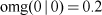
And for the angular filter is:

sita (0 | 0) = 0

(24)

sp (0 | 0) = 0.06

(25)

sr = 0.2, sq = 0.04

(26)

Where omg(0 | 0) sita(0 | 0) and are the optimal estimate of the initial sensor value, op(0 | 0) and op(0 | 0) are the initial weight, and they are easy to be fixed.

Get the sensor data which has been attenuated by the RC network, and load them to the Kalman filter in the MATLAB environment. Then the filtered signal curves, as shown in Fig. 9 and Fig. 10, can be accessed. In Fig. 9, the red curve is the filtered angular velocity curve, while the blue is the initial one. In the vicinity of 0.5s, a significant change of the curve is that the signal mutation caused by the shock disappears, and the same phenomenon exists in the angle sensor signal filtering, as shown in Fig. 10, this shows that the designed Kalman filter has played a filtering effect, attenuating the impact disturbance, this is what we expect. Another phenomenon exists in both Fig. 9 and Fig. 10 is the change of the phase or amplitude in the filtered curve. In Fig. 9 both have changed and some more changes of amplitude in Fig. 10, however, this is not a major problem, what we concern is the impact disturbance can be filtered by the filter, now our aim has been achieved and they can be weaken by adjusting the value of covariance to solve.

Figure 9.

Kalman filter testing for tilt angle rate

Figure 10.

Kalman filter testing for tilt angle

5.3. Testing of the hybrid controller

To contrast the effects with the smooth control method and the non-smooth control method, two sets of tests are given in this section. The first group is not loaded smooth controller, and the second is consisted of smooth control. In the two trials, the interference sources are both a rubber hammer. Because it is impossible to accurately control the force, the two groups interfering signal energy will be different, but we have tried to reduce the errors between them in the course of the experiment.

For the first test, the single states feedback gains are set as −1.83 for the tilt rate, −10.96 for the tilt angle and −9.63 for the robot speed. They are different from the second test; the reason is that in a non-smooth controller, the overlarge feedback gain is a direct reason of the system instability.

In the second test, the hybrid controller parameters are set as follows. For the partial states feedback controller, states feedback gain of the tilt angle, tilt angle rate and the robot velocity are −17.25, −7.25, −16.75; and for the PID controller the coefficients are 75 for proportional, 100 for integral and 50 for differential constant.

At the beginning of the first test the robot is in balance, exerting an instantaneous disturbance (in the experiment, we use the rubber hammer to hit shift to get the impact signal.), and then record all the data, import them to MATLAB then get the test curve, as shown in Fig. 11.

As can be seen from the experimental curves, when the robot is first under the impact disturbances, it will generate severe vibrations in 3 seconds department, especially the tilt angle rate (green curve in Fig. 11). Meanwhile, the output of angle sensor is severely distorted due to the vibrations, and distortion of the data will either lead to more serious vibration of the robot, or the robot under the controller gradually stabilized, which depends on the state feedback gains matrix. Although the robot will tend to stability in the selected feedback gains, the vibrations still exist when it is basically in the balance position. For the non-smooth controller, despite it can restore to balance position in about 3 seconds after the impact disturbance, vibrations exist in all of the control processing; such vibrations are not tolerated for the two-wheeled robot.

For the second test, the experiments process is the same as the first one, and the test curves are obtained as shown in Fig. 12, Fig. 13 and Fig. 14.

Figure 11.

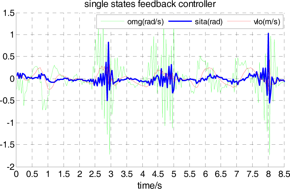
Non-smooth controller

Figure 12.

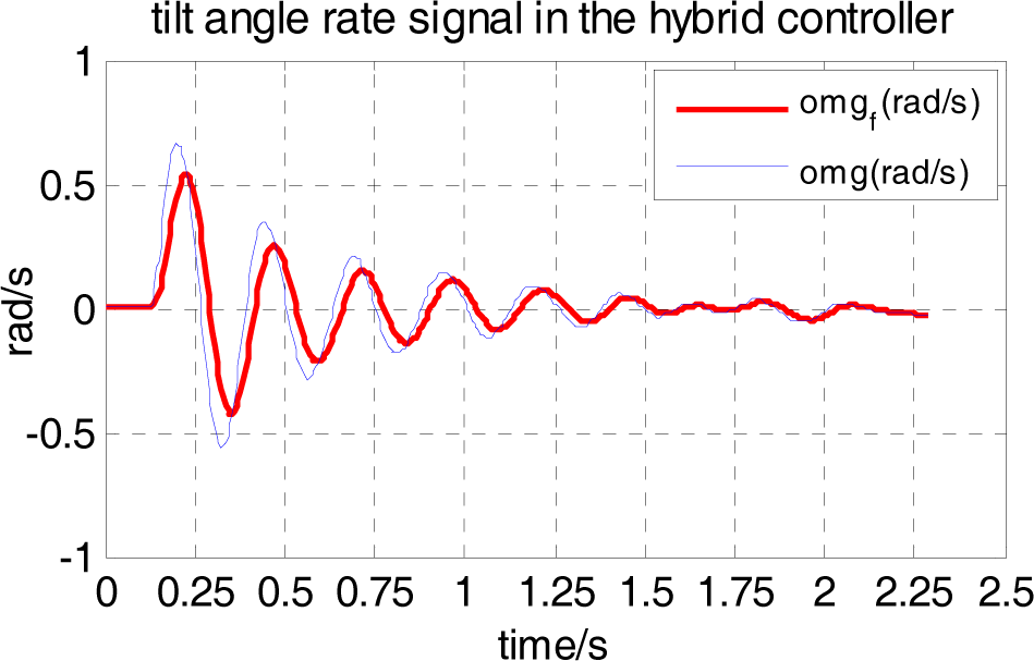
Tilt angle rate signals in the hybrid controller

Figure 13.

Tilt angle signals in the hybrid controller

It is clear that the robot can restore to balance in about 2s, under the impact disturbance from the test; when the impact signal is applied on the robot at about 0.1s, as shown in Fig. 13, the tilt angle has a significant mutation, the mutation signal is not really the point of the angle signal, but the acceleration sensor signal as the impact of the disturbance caused by the interference output, needs to be filtered or smoothed. The red curve, as shown in Fig. 13, shows that the Kalman filter on a signal through the RC network has a smoothing function so that the system under the impact of disturbances can realize smooth stable control.

The PID speed synchronized control effect, as shown in Fig. 14, shows good speed tracking performance analysis of the data by more than three hundreds groups, the speed deviation of algebra and only 0.037526 m/s, this can be seen from Fig. 15. The maxim speed error occurs at about 0.35s, and the value of it is approximately 0.07. In other sessions, error of plus or minus 0.03m/s or less, walk straight for two robots, the control precision can satisfy such requirements, after all, the ground situation in the case of inconsistencies do the complete wheel speed consensus is hardly realized.

Figure 14.

Two wheel speed of hybrid controller

Figure 15.

Velocity errors of the two wheels

7. Conclusion

A smooth control method for the two-wheeled self-balance robot under impact disturbances is proposed in this paper, and implementing of it is presented. Undamped frequency of the robot is researched and the cutoff frequency of the filters is got. A dual closed-loop controller based on partial states feedback and PID is then established, as well as a filter combined with RC network and Kalman filter. The blend controller is easy to implement and can achieve both the speed of the wheels coordinated control, and the impact disturbance signals can be maximally eliminated for a smooth control performance. From the experiments, the smooth control method is feasible and effective. Although the establishment of the state space model does not consider turning movement, the robot can achieve turning movement by changing the speed of two wheels.

8. Acknowledgment

This work was supported by National Hi-tech Research and Development Program of China (Grant No. 2008AA04Z208), and National Nature Science Foundation of China (Grant No. 60975070).

References

Ahmad

Tokbi

M. O.

(2009). “Rejection of Yaw Disturbance in a Two-Wheeled Wheelchair System.” 2009 Third Asia International Conference on Modelling & Simulation, Vols 1 and 2: 454–459 776.

Andary

Chemori

(2008). Stable limit cycle generation for underactuated mechanical systems, application: Inertia wheel inverted pendulum. Intelligent Robots and Systems, 2008. IROS 2008. IEEE/RSJ International Conference on.

Anderson

D. P.

(2007). “nBot.” from http://www.geology.smu.edu/∼dpa-www/robo/nbot/, [2007-7-1].

Ashokaraj

Silson

(2002). Application of an extended Kalman filter to multiple low cost navigation sensors in wheeled mobile robots. Sensors, 2002. Proceedings of IEEE.

Butler

L. J.

Bright

(2008). Feedback control of a self-balancing materials handling robot. 2008 10th International Conference on Control, Automation, Robotics and Vision (ICARCV 2008), 17–20 Dec. 2008, Piscataway, NJ, USA, IEEE.

Chen

(2003). Modeling random gyro drift by time series neural networks and by traditional method. Neural Networks and Signal Processing, 2003. Proceedings of the 2003 International Conference on.

Gans

N. R.

Hutchinson

S. A.

(2006). Visual Servo Velocity and Pose Control of a Wheeled Inverted Pendulum through Partial-Feedback Linearization. Intelligent Robots and Systems, 2006 IEEE/RSJ International Conference on.

Grasser

D'Arrigo

(2002). “JOE: A mobile, inverted pendulum.” IEEE Transactions on Industrial Electronics 49(1): 107–114.

Huang

J. A.

Guan

Z. H.

(2010). “Sliding-Mode Velocity Control of Mobile-Wheeled Inverted-Pendulum Systems.” Ieee Transactions on Robotics 26(4): 750–758.

10.

Imamura

Takei

(2008). Sensor drift compensation and control of a wheeled inverted pendulum mobile robot. Advanced Motion Control, 2008. AMC '08. 10th IEEE International Workshop on.

11.

Pathak

Franch

(2005). “Velocity and position control of a wheeled inverted pendulum by partial feedback linearization.” Ieee Transactions on Robotics 21(3): 505–513.

12.

Rong-Jong

Li-Jung

(2006). “Adaptive stabilizing and tracking control for a nonlinear inverted-pendulum system via sliding-mode technique.” Industrial Electronics, IEEE Transactions on 53(2): 674–692.

13.

Shiroma

Matsumoto

(1996). Cooperative behavior of a wheeled inverted pendulum for object transportation. Intelligent Robots and Systems '96, IROS 96, Proceedings of the 1996 IEEE/RSJ International Conference on.

14.

Widjaja

Shee

C. Y.

(2008). Kalman filtering of accelerometer and electromyography (EMG) data in pathological tremor sensing system. Robotics and Automation, 2008. ICRA 2008. IEEE International Conference on.

15.

Zhou

(2004). “The application of disturbance observer in two-wheeled mobile robot.” 2004 Ieee Conference on Robotics, Automation and Mechatronics, Vols 1 and 2: 171–174 1202.