Sage Journals: Discover world-class research

Abstract

This paper proposes a potential-based path planning algorithm of articulated robots with 2-DOF joints. The algorithm is an extension of a previous algorithm developed for 3-DOF joints. While 3-DOF joints result in a more straightforward potential minimization algorithm, 2-DOF joints are obviously more practical for active operations. The proposed approach computes repulsive force and torque between charged objects by using generalized potential model. A collision-free path can be obtained by locally adjusting the robot configuration to search for minimum potential configurations using these force and torque. The optimization of path safeness, through the innovative potential minimization algorithm, makes the proposed approach unique. In order to speedup the computation, a sequential planning strategy is adopted. Simulation results show that the proposed algorithm works well compared with 3-DOF-joint algorithm, in terms of collision avoidance and computation efficiency.

Keywords

path planning potential field articulated robot motion planning collision avoidance

1. Introduction

Path planning of a robot is to determine a collision free trajectory from its original location and orientation (called starting configuration) to goal configuration (Latombe, J. C. (1999)). Some planners adopt the configuration space (c-space) base approach (Lozano-Perez, T. (1983)) (Brooks, R. & Lozano-Preez, T. (1985)) (Kavraki, L.E. & Latombe, J.C. (1994)) (Kavraki, L.E., Svestka, P., Latombe, J.C., & Overmars, M. H. (1996)) (Tsourveloudis, N.C., Valavanis, K.P. & Herbert, T. (2001)) (Geraerts, R., & Overmars, M. H. (2007)) (Leng, C., Cao, Q.X. & Huang, Y.W. (2008)). A point in a c-space indicates a configuration of a robot which is usually encoded by a set of the robot's parameters; e.g., joint angles between the robot links. Thus, path planning of articulated robots is reduced to the problem of planning a path from the start to goal point in free space of the c-space. Unlike c-space based approaches, geometric algorithms directly use spatial occupancy information of the workspace (w-space) to solve path planning problem (Khosla, P. & Volpe, R. (1988)) (Chuang, J.H. & Ahuja N. (1998)) (Chuang, J.H. (1998)) (Valavanis, K.P., Herbert, T. & Tsourveloudis, N.C. (2001)) (Lin C.C. & Chuang, J.H. (2010)) (Tsai, C.H., Lee, J.S. & Chuang, J.H. (2001)) (Lin C.C., Pan, C.C. & Chuang, J.H. (2004)) (Lahouar, S., Zeghloul, S. & Romdhane, L. (2008)) (Dasgupta, B., Gupta, A., & Singla, E. (2009)) (Conkur, E.S. (2009)). Workspace-based algorithms usually extract relevant information about the free space and use them together with the robot geometry to find a path. However, not all approaches try to find path with minimum risk of collision. To minimize such a risk, repulsive potential fields between charged robot links and obstacles are used in (Khosla, P. & Volpe, R. (1988)) (Chuang, J.H. & Ahuja N. (1998)) (Chuang, J.H. (1998)) (Valavanis, K.P., Herbert, T. & Tsourveloudis, N.C. (2001)) (Tsai, C.H., Lee, J.S. & Chuang, J.H. (2001)) and (Lin C.C. & Chuang, J.H. (2010)) to match their shapes in the path planning.

In general, the potential function used to model the environment can be a scalar function of the distances between boundary points of the robot and those of obstacles. The gradient of such a scalar function, i.e., the repulsive force between the robot and obstacles, can be used to move the former away from latter making potential-based methods simple.

The Newtonian potential which is inversely proportional to the distance between two point charges is used in (Chuang, J.H. & Ahuja N. (1998)) for path planning in the 2-D space. The approach computes, similar to that done in electrostatics, repulsive force and torque between robots and obstacles in the workspace. An algorithm is developed to compute a safe and smooth object path by minimizing the potential function locally for obstacle avoidance, while the gross robot movement is subject to the constraints derived from the topology of the path given a priori. Since the potential is minimized for the obstacle avoidance purpose only, its local minima do not cause a problem in the path planning. The approach is generalized to the 3-D space for the path planning of rigid objects in (Tsai, C.H., Lee, J.S. & Chuang, J.H. (2001)) using the generalized potential proposed in (Chuang, J.H. (1998)).

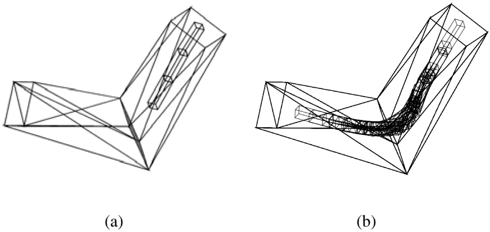
In Reference (Lin C.C., Pan, C.C. & Chuang, J.H. (2004)), a potential-based path planning algorithm was proposed for articulated robots with 3-DOF joints, spherical joints, as shown in Fig. 1(a). Because the joint has three DOFs, the robot can take full advantage of the proposed algorithm in potential minimization. In this paper, an improved algorithm is proposed for a robot with 2-DOF joints. While a robot with active 3-DOF joints is rare in practice, a robot with 2-DOF joints is often seen in many kinds of applications. The Hooke joint, which has two orthogonal rotation axes as shown in Fig. 1(b), is adopted in this paper to establish the connection between two links.

In this paper, the generalized potential field model presented in (Chuang, J.H. (1998)), is reviewed in next section, is adopted to model the workspace for the path planning of articulated robots. The proposed approach uses one or more guide planes (GPs) among obstacles in the free space as final or intermediate goals in the workspace for the articulated robot to reach. These GPs provide the articulated object a general direction to move forward and also help to establish certain motion constraints for adjusting robot configuration for minimum potential during path planning, as discussed in Section 3. An implementation of the proposed approach based on a sequential planning strategy is discussed. In Section 4, simulation results are presented for path planning performed for robots in different 3-D environments. Section 5 gives conclusions of this work.

Figure 1.

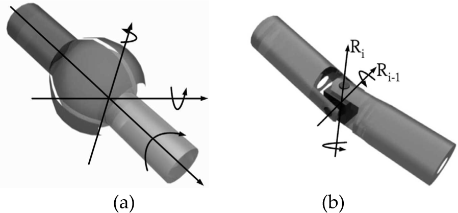
Two types of robot joint. (a) An example of 3-DOF joints, a spherical joint, and its axes. (b) An example of 2-DOF joints, a Hooke joint, and its axes

2. Generalized Potential Fields in the 3-D Space

In this paper, the generalized potential field proposed in (Chuang J.H. (1998)) is used to modal the 3-D environment by representing object/manipulators by charged sample points, and obstacles by charged polygons, respectively. The main advantages of using such a free space model include: (i) the repulsion among object, manipulators, and obstacles, in forms of force and torque, can be derived in closed form, (ii) the planned object/manipulator paths are spatially smooth and (iii) the collision avoidance of these paths are guaranteed if the above charged points are adequate.

In (Chuang, J.H. (1998)), the potential function is assumed to be inversely proportional to the distance between two point charges to the power of an integer (m). Thus, the potential field at point r due to a polygon S in the 3D space can be evaluated as

\int_{S} (d S / R^{m}) \begin{matrix} , \begin{matrix} m \geq 2 \end{matrix} \end{matrix}

(1)

Where R = |r' - r|, r' ∈ S, and integer m is the order of the potential function. In particular, it is shown that the repulsive force exerted on a point charge due to a 3-D polygon can be obtained analytically by evaluating the gradient of the potential function (for m=3)

\int_{S} \frac{d S}{R^{3}} \underline{\underline{Δ}} \sum_{i} [Φ_{3, i} (x_{2}^{i}, y_{2}^{i}, z) - Φ_{3, i} (x_{1}^{i}, y_{1}^{i}, z)] + \frac{α}{z}

(2)

with (subscript i is omitted(see Appendix))

Φ_{3} (x, y, z) = \frac{1}{z} \tan^{- 1} \frac{x z}{y \sqrt{x^{2} + y^{2} + z^{2}}},

(3)

where the xⁱ-yⁱ-z coordinate system is determined by the right-hand rule for each edge i of the polygon such that z is measured along the normal direction of S, and xⁱ is measured along edge i of the polygon, respectively, and α is a constant. Hence, if a robot is represented by charged points and obstacles are represented by charged polygons. The repulsive force exerted on the robot due to obstacles can be denoted as

\begin{array}{l} f = \sum_{i}^{m} (\sum_{j}^{n} f_{i_{x}}^{j}, \sum_{j}^{n} f_{i_{y}}^{j}, \sum_{j}^{n} f_{i_{z}}^{j}) \\ = \sum_{i}^{m} (\sum_{j}^{n} \frac{\partial Φ_{3, i}^{j}}{\partial x}, \sum_{j}^{n} \frac{\partial Φ_{3, i}^{j}}{\partial y}, \sum_{j}^{n} \frac{\partial Φ_{3, i}^{j}}{\partial z}) \end{array}

(4)

where m is the number of charged points, n is the number of obstacle polygons, and

\frac{\partial Φ_{3}}{\partial x} = \frac{y}{(x^{2} + y^{2}) \sqrt{x^{2} + y^{2} + z^{2}}},

(5)

\frac{\partial Φ_{3}}{\partial y} = \frac{- x (x^{2} + 2 y^{2} + z^{2})}{(x^{2} + y^{2}) (y^{2} + z^{2}) \sqrt{x^{2} + y^{2} + z^{2}}}

(6)

\begin{array}{l} \frac{\partial Φ_{3}}{\partial z} = \frac{\tan^{- 1} \frac{x z}{y \sqrt{x^{2} + y^{2} + z^{2}}}}{z^{2}} \\ \begin{matrix} \begin{matrix}  \end{matrix} \end{matrix} + \frac{x y (x^{2} + y^{2})}{z (x^{2} + y^{2}) (y^{2} + z^{2}) \sqrt{x^{2} + y^{2} + z^{2}}} \end{array}

(7)

The discussion for repulsive torque is similar and is omitted for brevity.

3. Path Planning Algorithm

In this section, the application of the potential model reviewed in the previous section to path planning of articulated robots with 2-D joints will be discussed. For a rough description of the path of an articulated robot, the proposed approach identifies one or more guide planes (GPs) as its final or intermediate goals in the 3-D workspace (see Fig. 2). The generation and selection of initial GPs will be discussed next. The GPs are polygons among obstacles in the free space, providing the articulated robot a general direction to move forward. As for a description of the configuration of the articulated robot, an n-link articulated robot is represented by its leading tip and the n-1 joints, as shown in Fig. 2. A sequential and collision free traversal of a given sequence of GPs by these control points (and the links) is regarded as a global solution of the path planning problem of the articulated robot. In the planning procedure discussed next, intermediate GPs will also be added along the path each time when a given GP is not directly reachable.

Figure 2.

An articulated robot with a leading tip, joints, links and a moving base is to move toward the goal by sequentially traversing a sequence of GPs.

3.1 Generation and Selection of initial GPs

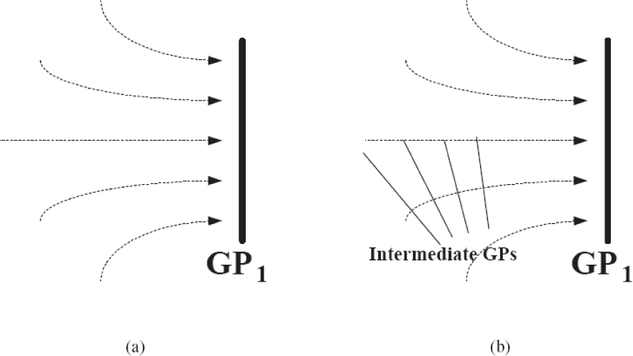
In the proposed algorithm, the GPs provide the articulated robot a general direction to move forward. The selection of the initial GPs may base on (i) their density along the passage, (ii) the visibility between two adjacent GPs, or (iii) the angular variation of two adjacent GPs. For the examples considered in this paper, the initial GPs are selected arbitrarily and the algorithm seems to work reasonably well in terms of the sensitivity of the planned path to the selection of initial GPs. In general, these initial GPs can also be obtained from the Generalized Cylinder (GC) (Nevatia, R. & Binford, T. O. (1977)) representation as cross-sections perpendicular to the GC axis (see Figs. 3(a) and (b)). Fig. 3(a) shows a passage which has an approximate rectangle cross-section, and an axis of its GC representation. Often, there is no limit on the number of cross-sections while their shapes are not specified in advance explicitly GC representation (see Fig. 3(b)).

Figure 3.

The generalized cylinder presentation of a passage

Figure 4.

Basic path planning procedure for a given GP (see text)

On the other hand, the shape of the GPs is usually not critical in the proposed approach as long as the GPs are confined in the free space. Thus, mainly the normal vectors of the GPs, e.g., obtained from the direction of the GC axis are important. Such an axial representation can also be derived from (i) the global navigation function as in (Connolly, C. I. & Grupen, R. A. (1990)) (Barraquand, J. & Latombe, J.C. (1991)) (Koditschek, D.E. (1987)), as well as (ii) the tree structure representation of free space obtained from the wavefront expansion presented in (Brock, Oliver & Kavraki, L. E. (2001)). While the gradient of (i) leads a point object to the goal, global connectively of free space is available in (ii) and is used in (Brock, Oliver & Kavraki, L. E. (2001)) to solve a planning problem in low dimensions.

While the idea of initial GPs can be regarded as a simplified version of global navigation functions which lead the robot to its final goal, the intermediate GPs added in Step 1 of Articulate_ Robot_to_GP is derived from a “local” navigation (potential) function in the proposed approach. Instead of leading the robot to the final goal (point), the potential field attracts the robot to an intermediate goal (plane), i.e., one of initial GPs. Thus, depending on its current location, the robot is allowed to reach an intermediate goal plane at various locations via various paths. Such flexibility in generating a global forward movement, compared to the traversal of the single path derived from a global navigation function, will hopefully reduce the number of collisions needed to be corrected, and thus the intermediate robot configuration, during the path planning.

3.2 Basic Procedure of Path Planning

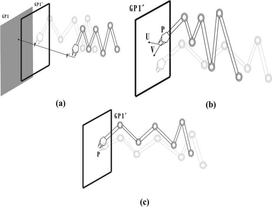
In this paper, the proposed path planning approach derives a series of minimum potential configurations along the path of an articulated robot by locally adjusting its configuration for minimum potential using the results reviewed in Sec. 2. Assuming that a guide plane GP₁ is given as an intermediate goal, the basic path planning procedure for moving the leading tip, p', of an articulated robot onto GP₁ include (see Fig. 4):

Translate links of the articulated robot to move p' toward the GP₁. If p' can not reach GP₁ directly, e.g., due to collision, an intermediate plane GP'₁ is inserted. (Fig. 4(a))

Search for the minimum potential configuration of the articulated robot for p ∈ GP'₁ by repeatedly executing:

(i) Search for the minimum potential configuration of the articulated robot with lnk₁ fixed in orientation

by sliding p on GP'₁ (see Fig. 4(b)). (ii) Search for the minimum potential configuration of the articulated robot with p fixed in position (see Fig. 4(c)).

(iii) Repeat (i) and (ii) until p reaches GP₁.

In general, there are different ways to change the configuration of the articulated robot to move p' toward GP₁. A simple translation of all links is adopted in (i) as a preliminary implementation of our algorithm, as shown in Fig. 4(a). The direction of the translation is determined such that $\vec{p}$ is in the direction of the attractive force $\vec{F_{p'}}$ , experience by p' due to GP₁. A collision check is performed for such a translation. If collision occurs, the distance of the translation is halved until the translation is collision-free. Accordingly, a new GP is inserted, e.g., GP'₁. No configuration improvement to reduce the repulsive potential is considered at this stage.

As for the search for the minimum potential configuration of the articulated robot in (ii), since lnk₁ has five DOFs, i.e., two for its location for p ∈ GP'₁ and three for its orientation, the associated constrained optimization problem is divided into two iterative univariant optimization procedures, as in (ii-a) and (ii-b). In (ii-a), lnk₁ is fixed in its orientation (see Fig. 4(b)) as p slides on GP'₁ to search for the minimal potential configuration and other links are sequentially adjusted in orientation, staring from lnk₂. In (ii-b), lnk₁ is adjusted in orientation while fixed in position (see Fig. 4(c)) and the procedure for adjusting the rest links is similar to that in (ii-a), except only two DOFs for orientation. For a particular GP, say GP'₁ in Fig. 4, (ii-a) and (ii-b) are repeatedly performed until negligible change in the configuration of the articulated robot is obtained. Then, another intermediate GP which is closer to GP₁ is obtained with (i) and the process repeats. The path planning algorithm, as summarized below, ends as the leading tip reaches the given GP₁ or exits abnormally for an infeasible problem. Detailed implementation of the algorithm is presented in the next subsection.

Algorithm Articulated Robot to GP

Step 0	Initialize δ = δ₀ and GP ← GP₁.
Step 1	Translate all links of the articulated robot with distance δ to move p' to p along $\vec{F_{p'}}$ . Find the smallest n 0 such that δ ← δ/2ⁿ corresponds to a feasible and collision-free translation. If δ < δ_min, go to Step 6; otherwise, construct GP'₁ with $G {P^{'}}_{1} ⊥ \vec{F_{p}}$ and p ∈ GP'₁, and let GP ← GP'₁.
Step 2	Translate lnk₁, by sliding p on GP, and adjust the orientations of the rest links to minimize the potential.
Step 3	With p fixed in position, adjust the orientations of all links to minimize the potential.
Step 4	Go to Step 2 if the translation in Step 2 or the joint angle adjustment in Step 3 is not negligible.
Step 5	If p reaches GP₁, the planning is completed. Otherwise, p' ← p and go to Step 1 with δ = δ₀.
Step 6	Exit and report that GP₁ is unreachable.

For path planning involving multiple GPs, the above algorithm will be executed for each of them sequentially. It is assumed that the planning for a GP starts as the planning of the previous GP is accomplished. The path planning ends as the leading tip of the articulated robot reaches the goal, which is usually a (goal) GP in the path planning problems considered in this paper.

3.3 Implementation Details

3.3.1 Initialization and Step 1 of Algorithm

In the initialization of Articulated_Robot_to_GP , the initial step size, δ₀, is arbitrarily chosen, i.e., δ₀ = 10% of workspace size. Generally, the number of robot configurations and the computation time depends on δ₀. For larger δ₀, fewer configurations will need to be calculated along the path if there is no collision. On the other hand, if δ₀ is too big the computation time may actually increase because collisions may occur frequently. A threshold, i.e., δ_min = 1% of workspace size, is established to set a lower bound of the magnitude of allowed translation. A translation which requires a smaller movement, δ < δ_min, indicates an infeasible path planning problem.

In Step 1 of algorithm, there are different ways to move p' toward GP₁. For example, p' can be moved toward GP₁ in the normal direction of GP₁. In our simulation, the articulated robot is translated, as a rigid object, to move the leading tip from p' to p by an distance δ along the direction of attraction, $\vec{F_{p'}}$ , as shown in Fig. 5(a). In the far field, $\vec{F_{p'}}$ has a near spherical symmetry and p' is attracted toward GP₁ as if GP₁ is a point attractor. In the near field, $\vec{F_{p'}}$ will lead p' toward GP₁ approximately in the normal direction of GP₁. In practice, since δ₀ is finite instead of infinitely small, p' may reach GP₁ at different locations from various directions.

While no configuration improvement to reduce the repulsive potential is considered in the above translation procedure, Steps 2 and 3 minimize the potential through constrained optimization procedures. To that end, an intermediate GP, GP'₁, is added along the path to serve as a geometric constraint for successive adjustments of the configuration of lnk₁. Again, as long as p ∈ GP'₁, the choice of the orientation of GP'₁ is not unique. For example, GP'₁ can be oriented such that it is parallel with GP₁. A more reasonable approach is adopted in our simulation wherein GP'₁ is chosen to be perpendicular to $\vec{F_{p'}}$ , as shown in Fig. 5(b). Thus, the direction of translation to minimize the potential in Step 2, as discussed next, is perpendicular to that of the translation in the next execution, if necessary, of Step 1.

3.3.2 Adjusting the leading tip position in Step 2

After the leading tip reaches p, as shown in Fig. 4(b), one of the univariant procedures to minimize the repulsive potential, which allows lnk_n to adjust its location but not its orientation, is performed in Step 2 of Articulated_Robot_to_GP . In order to speed up the computation, a sequential planning strategy (Gupta, K. K. (1990)) which plans the motion of links sequentially is adopted in Step 2. Accordingly, the procedures of Step 2 first minimize the potential of lnk₁ whose translation is constrained in two dimensions by GP. As for the motion of lnk_i (i > 1), as in (Gupta, K. K. (1990)), it is assumed that all links up to lnk_i-1 has been planned, i.e., one end of lnk_i is fixed in position. Therefore, only the orientation of lnk_i, which has two degrees of freedom, need to be adjusted for minimum potential.

Figure 5.

The moving direction of articulated robots and intermediate GPs (see text).

Consider the forces exerted on lnk₁, as shown in more detail in Fig. 6, since the minimization is constrained by p ∈ GP only the projection of the resultant force experienced by lnk₁ on GP is taken into account. Let f₁ be the repulsive force exerted on lnk₁ due to the repulsion between lnk₁ and the obstacles. For a univariant minimization approach, only one variable is adjusted at a time. To determine the direction in which lnk₁ should translate to slide p on GP to reduce the repulsive potential, the projection of the resultant force exerted on lnk₁ along an arbitrary $\vec{u} / / G P, f_{1 u}$ is calculated. A gradient-based binary search for the minimum potential location of p along $\vec{u}$ can then be performed. The initial step of sliding is arbitrarily chosen as 10% of the workspace size. If the movement of lnk₁ along $\vec{u}$ or f_1,u is negligible, e.g., the movement is smaller than 1% of workspace size, another minimization of potential along $\vec{v}$ , which is orthogonal to $\vec{u}$ , is performed to minimize f_1,v. Step 2 ends when two consecutive binary searches along the two orthogonal directions result in negligible movement of lnk₁. In this step, since the orientation of lnk₁ is not changed, lnk₂ can be connected directly, through pure translation, to lnk₁ before the potential minimizations through rotations with respect to the two orthogonal axes of the 2-DOF joint take place. As for lnk, i ⩾ 3, since the previous potential minimization may have changed the orientation of lnk_i-1, more involved connection process, other than the direct connection, as used for lnk₂, will need to be performed to ensure the intactness of the robot, as discussed next. Once the optimal configuration of lnk₁ is determined, the procedure for adjusting the rest links, except lnk₂, is similar to that in Step 3, as discussed later.

Consider joint J_i which connects two links, lnk_i and lnk_i-1, as shown in Fig. 1(b). Assume R_i-1 represents the rotation axis of lnk_i-1 after a potential minimization procedure while R^A_i is the rotation axis of lnk_i (which is to be connected to lnk_i-1 such that a potential minimization for lnk_i can take place), as shown in Fig. 7. Because of the constraint of the 2-DOF joint (R_i ⊥ R_i-1), lnk_i can not be connected directly to lnk_i-1 through pure translation if the orientation of lnk_i-1 has been changed due to potential minimization. Let S_i be the skeleton axis of lnk_i. It is obviously that two rotation axes are not always orthogonal if two links are connected arbitrarily. Such a configuration of these two links is illegal for a robot with 2-DOF joints. Therefore, R_i should be moved from R^A_i to R^B_i and then orthogonal to R_i-1. R^A_i can be determined as following. Assume all possible positions of R_i are lying on Plant P if lnk_i rotates about the axis S_i. R^⊥_i-1 is the projection of R_i-1 on P. If a vector R^B_i of P is orthogonal to R^⊥_i-1, it will be orthogonal to R_i-1 too. Thus, lnk_i should rotate about S_i by θ to let R_i moves to R_i^B. After the previous adjusting lnk_i orientation, the two links are connected legally with a 2 DOF joint. And, then, the further potential minimization can take place.

Figure 6.

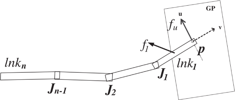
Translating lnk₁ to slide p on GP₁ to reduce the repulsive potential

Figure 7.

Since T_i-1 is perpendicular with T_i, the lnk_i should rotate with respect to S_i to let T'_i moves to T_i

3.3.2 Adjusting joint angle in Step 3

Once the minimum potential position of lnk_n is determined with Step 2 of Articulated_Robot_to_GP, another univariant procedure, which allows lnk₁ to adjust it sorientation with leading tip p fixed in position is performed to reduce the potential further, as shown in Fig. 4(c). Under such a constraint, lnk₁ can rotate with respect to p to reduce the repulsive potential. The direction in which lnk₁ should rotate is determined by the repulsive torque experienced by lnk₁ with respect to p.

Let τ₁ be the repulsive torque experienced by lnk₁ with respect to p due to the repulsion between lnk₁ and obstacles. To find the minimum potential orientation of lnk₁ for p fixed in position, gradient-based binary searches are performed repeatedly using the projection of τ₁ along three orthogonal axes of rotation, e.g., τ_1,u, τ_1,v and τ_1,w, respectively. For each binary search, the initial rotating angle is arbitrarily chosen as 5°, while the accuracy in identifying the 1-D potential minimum is chosen as 0.5°. Step 3 ends if a binary search results in a negligible change in the orientation of lnk₁, i.e., less than 0.5°. In this step, the rest links (lnk_i ∀i > 1), should be connected to lnk_i-1 legally, when the orientation of the lnk_i-1 is determined. The connection procedure is the same one in Step 2. Then, since there are only two rotation axes of a joint, rest links from lnk₂ to lnk_n adjust their orientation along the two axes, R_i and R_i-1, of J_i.

Figure 8.

A path planning example for a 3-link articulated robot in a 1-GP workspace. (a) The initial configuration. (b) The trajectory

4. Simulation Results

In this section, simulation results are presented for path planning performed on Pentium III (800MHz) personal computer for articulated robots in 3-D environments. Fig. 8(a) shows the initial configuration of the path obtained for a 3-link articulated robot in a 1-GP workspace wherein the GPs are shown as black polygons. Fig. 8(b) shows the complete trajectory of the articulated robot which reaches the final GP safely. Since collisions occur frequently near the 90 degrees turn of the passage for the δ₀ chosen, more configurations of the articulated robot are planned near the turn than those near start and goal. Due to the repulsive potential model, the trajectory of the articulated robot is smooth and lies near the middle of the workspace. The simulation takes a total of 42.466 seconds to plan the 14-configuration collision-free path.

Figs.9(a)(b) show the initial configuration and the trajectory, respectively, of the path obtained for another 3-link articulated robot in a 6-GP workspace. The simulation takes 91.34 seconds to planning the 23-configuration path. Since the twisted passage shown in Fig. 9 is a more narrow case than the case shown in Fig. 8, a longer time is needed to plan more robot configurations for the path. The planned path is also smoother spatially.

Figure 9.

A path planning example for a 3-link articulated robot in a 6-GP workspace. (a) The initial configuration. (b) The final trajectory

Figure 10.

A path planning example for a 4-link articulated robot in a 5-GP workspace. The initial configuration and the final trajectory.

Fig. 10 shows the initial conguration and final trajectory of the path obtained for a 4-link articulated robot moving in a turnaround passage. It can be seen clearly from Fig. 10 that the articulated robot traverses the five GPs safely and smoothly. The simulation takes a total of 155.19 seconds to plan the 17-configuration collision-free path. Since the passage of this example is more crooked, more intermediate GPs are added into the path, which in turn increases the computation time. However, the computation time of the same case for the 3D-joint robot is 151.52 seconds. The computation time of the 2D-joint robot does not increase significantly.

Fig. 11 shows the final trajectory of the path obtained for a 3-link articulated robot moving into a round-bottomed flask. The simulation takes 18.22 seconds to planning the 11-configuration path. It is easy to see that the robot move in the center of the flask.

Figure 11.

A path planning example for a 3-link articulated robot in a 4-GP workspace.

4.1 A Comparison Between 2-DOF Joints and 3-DOF Joints

In this section, the simulation results of the 2-DOF-joint algorithm are compared with the ones of 3-DOF-joints algorithm. In order to show the difference of paths derived by the two algorithms clearly, the third configurations of robots with 2-DOF joints and 3-DOF joints of Fig. 2 are shown in Figs. 13(a)(b), respectively. In Fig. 13(b), the second link is twisted to minimize the configuration potential due to the additional DOF, rotating with respect to the skeleton. In general, the algorithm with 2-DOF joints takes more time than a 3-DOF one to plan a collision-free path because the 2-DOF robot has less DOFs to minimize the potential. Figs. 14(a)(b) show trajectories of the example in Fig. 9 of the algorithms with 2-DOF joints and 3-DOF joints, respectively. While Fig. 14(a) takes 91.34 seconds to planning a 24-configuration path, Fig. 14(b) takes 88.16 seconds to planning an 18-configuration path. Since there are more motion constrain for the 2-DOF-joint robot, its algorithm plans more intermediate configurations to archive collision free. Since the 3-DOF-joint robot has additional DOFs to minimize potential than the 2-DOF one, the planned trajectory is more smoothly. As shown in Figs. 14, the difference between two trajectories of two algorithms is not significant.

Figure 13.

Two planned paths for a 3-link articulated robots with 2-DOF and 3-DOF Joints. (a) The third configuration of the robot with 2-DOF joints. (b) The third configuration of the robot with 3-DOF joints

Figure 14.

Two planned paths for a 3-link articulated robots with 2-DOF and 3-DOF Joints in the same environment.(a) A 24-configuration path of the robot with 2-DOF joints. (b) A 24-configuration path of the robot with 3-DOF joints

5. Conclusion

In this paper, a potential-based path planning of articulated robots with 2-DOF joints is proposed. Since a robot with 2-DOF joints is more trivial than 3-DOF joint robots in practice, the proposed algorithm is more adoptable than the 3-DOF-joint algorithm. In the proposed algorithm, a set of initial GPs are used to guide the robot moving toward. It is assumed that such a sequence of GPs to be traversed by an articulated robot is given in advance in the workspace providing the general direction of the path. According to the motion constraints established by the GPs, the proposed approach derives the path for the articulated robot by adjusting its configurations at different locations along the path to minimize the potential using the force and torque between links and obstacles. Simulation results show that the planned path is similar to the planned path derived by the 3-DOF-joint algorithm and the computation time does not increase significantly.

6. Appendix

In this section, the generalized potential model (Chuang, J.H. (1998)) is reviewed. Consider a planar surface S in the 3-D space, the direction of its boundary, ΔS, is determined with respect to its surface normal, n̂, by the right-hand rule, û x l̂ = n̂, where û and l̂ are along the (outward) normal and tangential directions of ΔS, respectively. For the generalized potential function, the potential value at r is defined as (1). The Newtonian potential (m=1) is harmonic in the 3-D space and can not prevent the robot from colliding the obstacles, and thus can not be used for collision avoidance. The basic procedure to evaluate the potential at r can be summarized as follows:

Write the integrand of the potential integral over S as surface divergence of some vector function.

Transform the integral into the one over ΔS based on the surface divergence theorem.

Evaluate the integral as the sum of line integrals over edges of ΔS.

Without the loss of generality, it is assumed that

d \overset{Δ}{=} \hat{n} \cdot (r - r^{'}) > 0

(8)

which is equal to the distance from r to Q. For (i), we have

\frac{1}{R^{m}} = \nabla_{S} \cdot (f_{m} (R) P)

(9)

where P is the position vector of r' with respect to the projection of r on Q, r_Q, and

\begin{array}{l} f_{m} (R) = \frac{1}{P^{2}} \int R^{m - 1} d R \\ = {\begin{matrix} \frac{\log R}{R^{2} - d^{2}}, \\ \frac{- 1}{(m - 2) R^{m - 2} (R^{2} - d^{2})}, \end{matrix} \begin{matrix} \begin{matrix} m = 2 \\ m \neq 2 \end{matrix} \end{matrix} \end{array}

(10)

Note that if r_Q is inside S, f_m(R) will becomes singular for some r” = r_Q, (and R = d). Let Sɛ denote the intersection of S and a small circular region on Q of radius ɛ and centered at r_Q, the potential due to S can be evaluated as

\begin{array}{l} \int_{S} \frac{d S}{R^{m}} = \lim_{ε \to 0} [\int_{S - S_{ε}} \nabla_{S} \cdot (f_{m} (R) P) d S + \int_{S_{ε}} \frac{d S}{R^{m}}] \\ = \int_{Δ S} f_{m} (l) P \cdot \hat{u} d l + \lim_{ε \to 0} [- \int_{0}^{ε} ε^{2} f_{m} (\sqrt{ε^{2} + d^{2}}) d θ + \int_{0}^{α} \int_{0}^{ε} \frac{p d p d θ}{{(p^{2} + d^{2})}^{\frac{m}{2}}}] \\ = \sum_{i} P_{i}^{0} \cdot {\hat{u}}_{i} \int_{C_{i}} f_{m, i} (l_{i}) d l + g_{m} (α), \end{array}

(11)

where

\begin{array}{l} f_{m, i} (l_{i}) = f_{m} (R = \sqrt{l_{i}^{2} + d^{2} + {(P_{i}^{0})}^{2}}), \\ g_{m} (α) = {\begin{matrix} α \log d, \\ \frac{α}{(m - 2) d^{m - 2}}, \end{matrix} \begin{matrix} m = 2 \\ m \neq 2 \end{matrix} \end{array}

(12)

Pi0 is the distance between r_Q and C_i, li is measured from the projection of r on C_i along the direction of l̂_i, and α is the angular extent of the circumference of Sɛ lying inside S as ɛ -> 0. For m=3, we have

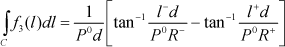
\int_{C} f_{3} (l) d l = \frac{1}{P^{0} d} [\tan^{- 1} \frac{l^{-} d}{P^{0} R^{-}} - \tan^{- 1} \frac{l^{+} d}{P^{0} R^{+}}]

(13)

with R⁻ and R⁺ equal to the distances from r to the two end points of C_i, respectively. Thus, the repulsive force exerted on a point charge due to S can be found analytically by evaluating the gradient of the following function

Φ_{3} (x, y, z) = \frac{1}{z} \tan^{- 1} \frac{x z}{y \sqrt{x^{2} + y^{2} + z^{2}}}

(14)

at some (x, y, z)'s.

7. Acknowledgments

This work is supported by National Science Council of Taiwan under grant no. NSC 98-2220-E-224-009 and NSC 98-2220-E-224-007.

References

Barraquand

Latombe

J.C.

(1991). Robot motion planning: A distributed representation approach, International Journal of Robotics Research, Vol. 10, No. 6, pp. 628–649, 1991.

Brock

Oliver

Kavraki

L. E.

(2001). Decomposition-based motion planning: A framework for real-time motion planning in high-dimensional configuration spaces, IEEE International Conference of Robotics and Automation, pp. 1469–1474, 2001.

Brooks

Lozano-Preez

(1985). A subdivision algorithm in configuration space for findpath with rotation, IEEE Transation on System, Man, Cybernetics, Vol. 15, No. 2, pp. 224–233, 1985.

Chuang

J.H.

(1998). Potential-based modeling of three-dimensional workspace of the obstacle avoidance, IEEE Transation on Robotics and Automation, Vol. 14, No. 5, pp. 778–785, 1998.

Chuang

J.H.

Ahuja

(1998). An analytically tractable potential field model of free space and its application in obstacle avoidance, IEEE Transation on System, Man, Cybernetics, Part B: Cybernetics, Vol. 28, No. 5, pp. 729–736, 1998.

Conkur

E.S.

(2009). Path Planning Using Potential Field for Highly Redundant Manipulators, Robotics and Autonomous System, Vol. 57, No. 2, pp. 194–201.

Connolly

C. I.

Grupen

R. A.

(1990). Path planning using laplace's equation, IEEE International Conference of Robotics and Automation, pp. 2102–2106, 1990.

Dasgupta

Gupta

Singla

(2009). A Variational Approach to Path Planning for Hyperredundant Manipulators, Robotics and Autonomous Systems, Vol. 57, No. 2, pp. 194–201.

Geraerts

Overmars

M. H.

(2007). Reachability-Based Analysis for Probabilistic Roadmap Planners, Robotics and Autonomous Systems, Vol. 55, No. 11, pp. 824–836.

10.

Gupta

K. K.

(1990). Fast collision avoidance for manipulator arms: A sequential search strategy, IEEE Transation on Robotic and Automation, Vol. 6, No. 5, pp. 522–532, Oct. 1990.

11.

Kavraki

L.E.

Latombe

J.C.

(1994). Randomized preprocessing of configuration space for fast path planning: Articulated robots, Proceeding IEEE/RSJ International Conference on Intelligent Robots and System, pp. 1764–1772, 1994.

12.

Kavraki

L.E.

Svestka

Latombe

J.C.

Overmars

M. H.

(1996). Probabilistic roadmaps for path planning in high-dimensional configuration spaces, IEEE Transation on Robotics and Automation, Vol. 12, No. 4, pp. 566–580, Aug. 1996.

13.

Khosla

Volpe

(1988). Superquadric artificial potentials for obstacle avoidance and approach, Proceeding IEEE International Conference on Robotics and Automation, pp. 1778–1784, 1988.

14.

Koditschek

D.E.

(1987). Exact robot navigation by means of potential functions: Some topological considerations, IEEE International Conference of Robotics and Automation, pp. 1–6, 1987.

15.

Lahouar

Zeghloul

Romdhane

(2008). Real-Time Path Planning for Multi-DoF Manipulators in Dynamic Environment, International Journal of Advanced Robotic Systems, Vol. 3, No. 2, pp. 125–132, 2008.

16.

Latombe

J.C.

(1991). Robot Motion Planning, MA: Kluwer, Boston, 1991.

17.

Latombe

J.C.

(1999). Motion planning: A journey of robots, molecules, digital actors, and other artifacts, The International Journal of Robotics Research, Vol. 18, No. 11, pp. 1119–1128, 1999.

18.

Leng

Cao

Q.X.

Huang

Y.W.

(2008). A Motion Planning Method for Omnidirectional Mobile Robot Based on the Anisotropic Characteristics, International Journal of Advanced Robotic Systems, Vol. 5, No. 4, pp. 327–340, 2008.

19.

Lin

C.C.

Chuang

J.H.

(2010). A Potential-Based Path Planning Algorithm for Hyper-Redundant Manipulators, Journal of the Chinese Institute of Engineers, Vol. 33, No. 3, pp. 415–427, 2010.

20.

Lin

C.C.

Pan

C.C.

Chuang

J.H.

(2004). A Novel Potential-Based Path Planning of 3-D Articulated Robots with Moving Bases, Robotica, Vol. 22, No. 4, pp. 359–367, 2004.

21.

Lozano-Perez

(1983). Spatial planning: A configuration space approach, IEEE Transation on Computers, Vol. C-32, No. 2, pp. 108–120, 1983

22.

Nevatia

Binford

T. O.

(1977). Description and recognition of curved objects, Artificial Intelligence, Vol. 8, No. 1, pp. 77–98, 1977

23.

Tsai

C.H.

Lee

J.S.

Chuang

J.H.

(2001). Path planning of 3-D objects using a new workspace model, IEEE Transation on System, Man, Cybernetics, Part B: Cybernetics, Vol. 31, No. 3, pp. 405–410, 2001.

24.

Tsourveloudis

N.C.

Valavanis

K.P.

Herbert

(2001). Autonomous vehicle navigation utilizing electrostatic potential fields and fuzzy logic, IEEE Transation on Robotics and Automation, Vol. 17, No. 4, pp. 490–497, 2001.

25.

Valavanis

K.P.

Herbert

Tsourveloudis

N.C.

(2001). Mobile robot navigation in 2-D dynamic environments using electrostatic potential fields, IEEE Transation on System, Man, Cybernetics, Part A: Systems and Humans, Vol. 30, No. 2, pp. 187–196, 2001.

A Path Planning Algorithm Using Generalized Potential Model for Hyper-Redundant Robots with 2-DOF Joints

Abstract

Keywords

1. Introduction

2. Generalized Potential Fields in the 3-D Space

3. Path Planning Algorithm

3.1 Generation and Selection of initial GPs

3.2 Basic Procedure of Path Planning

3.3 Implementation Details

3.3.1 Initialization and Step 1 of Algorithm

3.3.2 Adjusting the leading tip position in Step 2

3.3.2 Adjusting joint angle in Step 3

4. Simulation Results

4.1 A Comparison Between 2-DOF Joints and 3-DOF Joints

5. Conclusion

6. Appendix

7. Acknowledgments

References