Sage Journals: Discover world-class research

Abstract

The terms bioaccumulation and bioconcentration refer to the uptake and build-up of chemicals that can occur in living organisms. Experimental measurement of bioconcentration is time-consuming and expensive, and is not feasible for a large number of chemicals of potential regulatory concern. A highly effective tool depending on a quantitative structure-property relationship (QSPR) can be utilized to describe the tendency of chemical concentration organisms represented by, the important ecotoxicological parameter, the logarithm of Bio Concentration Factor (log BCF) with molecular descriptors for a large set of non-ionic organic compounds. QSPR models were developed using multiple linear regression, partial least squares and neural networks analyses. Linear and non-linear QSPR models to predict log BCF of the compounds developed for the relevant descriptors. The results obtained offer good regression models having good prediction ability. The descriptors used in these models depend on the volume, connectivity, molar refractivity, surface tension and the presence of atoms accepting H-bonds.

Keywords

BCF non-ionic organic compounds structure property relationships (QSPR)partial least square (PLS)principal components artificial neural networks (PC-ANN)

Introduction

Bioaccumulation is the process where the chemical concentration in an aquatic organism achieves a level exceeding that in the water, as a consequence of chemical uptake through all means of chemical exposure (e.g. dietary absorption, transport across the respiratory surface, dermal absorption, and inhalation). Bioconcentration is defined as the absorption of a chemical concentrations in an aquatic organism's tissues that is greater than that in the water as a result of exposure of the organism to a chemical concentration in the water via non-dietary routes. The extent to which a contaminant will concentrate in an organism is articulated as BCF which is the ratio of the chemical concentration in the organism (C_B) and the water (C_w)1:

BCF = C_{B} {/C}_{W}

(1)

Within a species, BCFs vary for different chemical compounds. The BCF of a chemical is the result of four processes: Absorption, Distribution, Metabolism and Excretion (ADME).² Bioconcentration is usually derived under laboratory conditions where the chemical is absorbed from the water via the respiratory surface and/or the skin only. Generally, the experimental measurement of bioconcentration is time-consuming and expensive, and is not feasible for a large number of chemicals of potential regulatory concern. For this reason attention is turning to estimation of BCF values by QSPRs. BCF values can be estimated from the octanol/water partition coefficient (K_ow) using QSPR models. In addition, K_ow values, either experimentally determined or estimated, can be used directly to assess the potential for bioaccumulation.

QSPRs are usually observed between log BCF and log K_ow. The majority of these are linear regression models^3–8 which give satisfactory results only for chemicals with log K_ow < 6, while for highly hydrophobic chemicals (log K_ow > 6), non-linear,^9,10 bilinear^11,12 or polynomial¹³ relationships have been proposed and applied for more satisfactory BCF prediction/estimation. Zhao et al¹⁴ performed a QSPR study on a large set of 473 compounds that was created with ISIS BASE 2.5 SP2. Lu¹⁵ proposed models for the prediction of BCF using connectivity indices and comprising experimental BCF data in fish (at steady-state) for 239 non-ionic organic compounds. This approach was applied by Gramatica and Papa^16,17 with the same data set previously modeled by Lu¹⁵ using a large starting set of theoretical molecular descriptors and by applying a genetic algorithm (GA) approach as the variable subset selection method to obtain multilinear regression models with few variables correlated with BCF. Fatemi et al¹⁸ reported a QSAR study on a set of 53 compounds using geometric, electronic and topological descriptors by artificial neural networks (ANN) to predict the value of log BCF for some compounds. Recently, a QSAR model for fish BCFs of 8 groups of compounds was developed employing partial least squares (PLS) regression, based on linear solvation energy relationship (LSER) theory and theoretical molecular structural descriptors.^19–21

Khadikar et al²² reported QSAR study on the estimation of bioconcentraction factor of polyhaloge-nated biphenyls using a distanced-based index called Padmakar-Ivan index, abbreviated as PI. Incited by these results, we have used the molecular descriptors used by Lu et al¹⁵ Gramatica and Papa^16,17 and Khadikar et al²² in addition to large set of other topological indices to model the BCF. It is worth to mention that, to our knowledge and to date, no attempt has been made to investigate neural network modeling using principal components for prediction of BCFs of the set of nonionic organic compounds.

Before discussing our results it is necessary to mention that both Lu et al¹⁵ and Gramatica and Papa in^16,17 used the same data set of 238 compounds, while Khadikar et al²² used only 16 polyhalogenated biphenyls from the original set of 238 compounds reported by Lu et al.¹⁵ Furthermore, Gramatica and Papa^16,17 did not verify the data and only deleted acrolein from the original data set reported by Lu et al.¹⁵ In this contribution, we observed that 9 compounds (compounds: 210-215, 218, 220, and 234) out of the larger set of 238 compounds need to be removed in order to obtain excellent models. The main reason for removing these 9 compounds is that the molecular descriptors used by us failed to establish structure-property relationship.

In view of the above, we used principal components–-artificial neural networks (PC-ANN) and PLS methods on the data set of 229 non-ionic compounds modeled by Lu et al.¹⁵ The proposed models were checked for their internal and external predictive power using cross validation parameters.

Experimental

Software

Geometry Optimization was performed by HyperChem (Version 7.0 Hypercube, Inc) at the AM1 level. Descriptors were calculated using HyperChem and Dragon software.²³ SPSS Software (version 13.0, SPSS, Inc.) was used for the simple multiple linear regression (MLR) analysis. PCA, ANN and PLS regression were performed in the MATLAB (Version 7.0.1 (R14), Mathworks, Inc.) environment.

Chemical data and descriptors

Compounds name and their BCFs are included in Table 1. Chemical structure of these compounds was obtained from HyperChem software and optimized on AM1 semi-empirical level. An AM1 optimization was chosen since it was developed and parameterized for common organic structures. The Optimization was preceded by the Polak-Rebiere algorithm to reach 0.01 root mean square gradient. In this study, 24 molecular descriptors including topological, 2D-autocorrelation, GETAWAY, properties and functional groups descriptors were calculated using HyperChem and Dragon software, see Abbreviations.

Table 1

Non-ionic organic compounds used in this study and their experimental log BCF values.

No.	Compound name	Log BCF
1	1,2-Dichloroethane	0.30
2^b	Trichloromethane	0.78
3	1,1,2,2-Tetrachloroethane	0.90
4	Trichloroetheylene	1.59
5	1,1,1-Trichloroethane	0.95
6^b	Tetrachloroetyelene	1.74
7	Tetrachloromethane	1.48
8	Pentachloroethane	1.83
9	Hexachloroethane	2.92
10	1,1,2,3,4,4-Hexachloro-1, 3-Butadiene	3.83
11	Benzene	0.64
12	Toulene	1.12
13^b	Styrene	1.13
14	Ethylebenzene	1.19
15^b	o-Xylene	1.24
16	m-Xylene	1.27
17	p-Xylene	1.27
18	p-Methyle styrene	1.50
19	m-Methyle styrene	1.55
20	Isopropylebenzene	1.55
21	2-Phenyledodecane	2.65
22^b	Octachlorostyrene	4.52
23	Napthalene	1.64
24	Acenaphtylene	2.58
25	Acenaphtalene	2.59
26	Biphenyle	2.64
27	Anthracene	2.83
28	2-Methylenapthalene	3.20
29^b	Fluorene	3.23
30	Phenanthrene	3.42
31	Benzo[a]pyrene	3.42
32^b	Pyrene	3.43
33	2-Methylephenanthrene	3.48
34	2-Chlorophenanthrene	3.63
35	9-Methylanthracene	3.66
36	Benzo[a]anthracene	4.00
37^b	Chlorobenzene	1.85
38	1,2-Dichlorobenzene	2.48
39	1,4-Dichlorobenzene	2.52
40	1,3-Dichlorobenzene	2.65
41	1,2,3-Trichlorobenzene	3.11
42^b	1,2,4-Trichlorobenzene	3.26
43	1,2,3,5-Tetrachlorobenzene	3.36
44	1,3,5-Trichlorobenzene	3.38
45	1,2,4,5-Tetrachlorobenzene	3.76
46	1,2,3,4-Tetrachlorobenzene	3.77
47^b	Pentachlorobenzene	3.86
48	2,4,5-Trichlorotoulene	3.87
49	Hexachlorobenzene	4.26
50	Bromobenzene	1.70
51	1,3-Dibromobenzene	2.80
52^b	1,2,3-Tribromobenzene	2.83
53	Hexabromobenzene	3.04
54	1,2-Dibromobenzene	3.10
55	1,2,4-Dibromobenzene	3.66
56^b	1,2,4,5-Tetrabromobenzene	3.79
57	1,3,5-Tribromobenzene	3.85
58	Octachloronapthalene	3.44
59	1,4-Dichloronapthalene	3.56
60	2-Monochloronapthalene	3.63
61^b	1,8-Dichloronapthalene	3.79
62	2,3-Dichloronapthalene	4.04
63	2,7-Dichloronapthalene	4.04
64	1,2,3,4-Tetrachloronapthalene	4.10
65	1,3,5,8-Tetrachloronapthalene	4.40
66^b	1,3,7-Trichloronapthalene	4.43
67	1,3,5,7-Tetrachloronapthalene	4.53
68	4-Chlorobipheyl	2.69
69	2,2′-Dichlorobiphenyl	3.26
70	4,4′-Dichlorobiphenyl	3.28
71^b	2,2′,4,4′,6-Pentachlorobiphenyl	3.37
72	2,4′-Dichlorobiphenyl	3.55
73	2,4′,5-Trichlorobiphenyl	3.75
74	3,5-Dichlorobiphenyl	3.78
75	2,2′,6,6′-Tetrachlorobiphenyl	3.85
76^b	3,3′,4,4′-Tetrachlorobiphenyl	3.90
77	2,2′,4,4′-Tetrachlorobiphenyl	4.02
78	2,4,5-Trichlorobiphenyl	4.02
79	2,2′,3,3′,4,4′,5,5′,6,6′-Decachlorobiphenyl	4.02
80	2,5-Dichlorobiphenyl	4.20
81^b	2,2′,3,3′-Tetrachlorobiphenyl	4.23
82	2,3-Dichlorobiphenyl	4.25
83	2,2′,5-Trichlorobiphenyl	4.27
84	2,4,4′-Trichlorobiphenyl	4.63
85	2,3′,4′,5-Tetrachlorobiphenyl	4.77
86^b	2,2′,4,4′,5,5′-Hexachlorobiphenyl	4.83
87	2,2′,3,5′-Tetrachlorobiphenyl	4.84
88	2,2′,4,5′-Tetrachlorobiphenyl	4.84
89	2,2′,5,5′-Tetrachlorobiphenyl	4.87
90	2,2′,4,4′,6,6′-Hexachlorobiphenyl	4.93
91^b	2,2′,4,5-Tetrachlorobiphenyl	5.00
92	2,2′,3,3′,4,4′,5,5′-Octachlorobiphenyl	5.08
93	2,2′,3,4,5′-Pentachlorobiphenyl	5.38
94	2,2′,4,5,5′-Pentachlorobiphenyl	5.40
95	2,2′,3′,4,5-Pentaclorobiphenyl	5.43
96^b	2,2′,3,3′,6,6′-Hexachlorobiphenyl	5.43
97	2,2′,3′,5,5′,6′-Hexachlorobiphenyl	5.54
98	2,2′,3,3′,4,4′,5,5′,6,-Nonachlorobiphenyl	5.71
99	2,2′,3,3′,4,4′-Hexachlorobiphenyl	5.77
100	3,3′,4,4′,5′-Pentachlorobiphenyl	5.81
101^b	2,2′,3,4,5,5′-Hexachlorobiphenyl	5.81
102	2,2′,3,3′,5,5,6,6′-Octachlorobiphenyl	5.82
103	2,2′,3,4,4′,5,6′-Heptachlorobiphenyl	5.84
104	2,2′,3,4,4′,5′-Hexachlorobiphenyl	5.88
105	2,2′,3,3′,4′,5,5′,6-Octachlorobiphenyl	5.88
106^b	2,2′,3,3′,4,4′,5,6-Octachlorobiphenyl	5.92
107	2,2′,3,4,5,5′,6′-Heptachlorobiphenyl	5.93
108	3,3′,4,4′,5,5′-Hexachlorobiphenyl	5.97
109	2,4,6-Tribromobiphenyl	3.93
110	2,2′,4,4′,6,6′-Hexabromobiphenyl	3.96
111^b	4,4′-Dibromobiphenyl	4.19
112	2,2′,5,5′-Tetrabromobiphenyl	4.80
113	2,7-Dichlorodobenzo-p-dioxin	2.13
114	1,2,4-Trichlorodibenzo-p-dioxine	2.36
115	1,2,3,4-Tetrachlorodibenzo-p-dioxine	2.55
116	Octachlorodibenzo-p-dioxine	2.76
117^b	2,8-Dichlorodibenzo-p-dioxine	2.82
118^b	1,2,3,4,6,7,8-Heptachlorodibenzo-p-dioxine	3.16
119	1,2,3,4,7-Pentachlorodibenzo-p-dioxine	3.21
120	1,2,3,7-Tetrachlorodibenzo-p-dioxine	3.24
121	1,3,6,8-Tetrachlorodibenzo-p-dioxine	3.36
122	1,2,3,4,7,8-Hexachlorodibenzo-p-dioxine	3.54
123^b	Dibenzo(1,4)dioxine	3.85
124	2,3,7,8-Tetrachlorodibenzo-p-dioxine	4.06
125	1,2,3,7,8-Pentachlorodibenzo-p-dioxine	4.50
126	Benzo[b]furan	2.56
127	Octachlorodibenzofuran	2.94
128^b	Dibenzofuran	3.34
129	2,3,7,8-Tetrachlorodibenzofuran	3.53
130	1,2,3,4,6,7,8-Heptachlorodibenzofuran	3.62
131	2,3,4,7,8-Pentachlorodibenzofuran	4.03
132	4-Cyanophenol	0.91
133^b	2-Methylphenol	1.03
134	Phenol	1.24
135	3-Chlorophenol	1.25
136	2,4-Dichlorophenol	1.50
137	4-Bromophenol	1.56
138^b	p-sec-Butylphenol	1.57
139	Hydroquinone	1.60
140	2,6-Dibromo-4-cyanophenol	1.67
141	4,6-Dichloroguaiacol	1.74
142	4-t-Butyylphenol	1.86
143^b	4,5,6-Trichloroguaiacol	1.97
144	4,5-Dichloroguaiacol	2.03
145	2,3,5,6-Tetrachlorophenol	2.15
146^b	2,4-Dimethylphenol	2.18
147	2-Chlorophenol	2.33
148	3,4,5-Trichloroguaiacol	2.41
149	2,4,6-Trichlorophenol	2.43
150	p-Nonyl phenol	2.45
151	Tetrachloroguaiacol	2.71
152^b	2,4,6-Tribromophenol	2.71
153	Pentachlorophenol	2.74
154^b	p-Dodecyl phenol	3.78
155	4-Chloroaniline	0.23
156	3-Chloroaniline	0.34
157	Aniline	0.41
158^b	2-Chloroaniline	0.57
159	Diphenylamine	1.48
160	3,4-Dichloroaniline	1.48
161	2,4-Dichloroaniline	1.98
162	N-Phenyl-2-napthylamine	2.17
163^b	2,3,4-Trichloroaniline	2.31
164	2,4,5-Trichloroanaline	2.61
165	2,3,4,5-Tetrachloroaniline	2.69
166	3,4,5-Trichloroaniline	2.70
167	2,4,6-Trichloroaniline	2.73
168^b	3,3′-Dichlorobenzidine	2.79
169	2,3,5,6-Tetrachloroaniline	3.03
170	Pentachloroaniline	3.17
171	Ethyl acetate	1.48
172	Dimethyl phtalate	1.76
173^b	Diethyl phtalate	2.07
174	Bis(2-ethylehexyl)phalate	2.34
175^b	Deltamethrin	2.66
176	Fenalerate	2.79
177	Benzyl butyl phatalate	2.89
178	Cypermethrine	2.91
179^a	2-t-Butoxy ethanol	-0.22
180	t-Butyl methyl ether	0.18
181^a	t-Butyl isopropylether	0.76
182	Bis(2-chloroethyl)ether	1.04
183	2,4,6-Trichloroanisole	2.94
184	2,4,6-Tribromoanisole	2.94
185	Methoxychlore	3.10
186^b	2,4,5-Trichlorodiphenyle ether	4.18
187	3,3′,4,4′-Tetrachlorodiphenyl ether	4.51
188	2-Methyl-4,6-dinitrophenol	0.16
189	4-Nitroaniline	0.64
190	2-Nitroaniline	0.91
191^b	3-Nitroaniline	0.92
192	3-Nitrophenol	1.40
193	2-Nitrophenol	1.60
194	2,4,5-Trichloronitrobenzene	1.84
195	3-Chloronitrobenzene	1.89
196^b	2,3,4,5-Tetrachloronitrobenzene	1.89
197	4-Chloronitrobenzene	2.00
198	2,5-Dichloronitrobenzene	2.05
199	2,4-Dichloronitrobenzen	2.07
200	3,4-Dichloronitrobenzene	2.07
201^b	2-Chloronitrobenzene	2.10
202	2,3-Dichloronitrobenzene	2.16
203	2,3,4-Trichloronitrobenzene	2.20
204	3,5-Dichloronitrobenzene	2.23
205	Pentachloronitrobenzene	2.40
206^b	2,4,6-Trichloronitrobenzene	2.88
207	Chloronitrofen	3.04
208	2,3,5,6-Tetrachloronitrobenzene	3.20
209	Phenthoate	1.56
210	Fenthion	2.68
211^b	EPN	3.05
212	Leptophos	3.78
213	Carbaryl	1.22
214	Molinate	1.41
215	BPMC	1.41
216	Acrylonitrile	1.68
217	Thiobencarb	2.03
218	Acridine	2.61
219^b	Lindane	2.84
220	B-HCH	2.86
221	α-HCH	2.95
222	Hexachlorocyclopentadiene	3.09
223	Xanthene	3.62
224^b	Dieldrine	3.71
225	Heptachlore	4.14
226	o-p′-DDT	4.57
227	Chlordane	4.58
228	p, p-DDE	4.71
229	p, p′-DDT	4.84

Compounds were considered as outliers;

Compound classified in the test set.

MLR analysis

MLR analysis using the method of maximum -R² with stepwise selection and elimination of variables²⁴ was employed to model the logarithm of the BCF (log BCF) relationships with different set of descriptors to select initial input models for the artificial neural networks algorithm (ANN).

PC-ANN

Principal component analysis (PCA) and more specifically factor analysis (FA) groups together variables that are collinear to form a composite indicator capable of capturing as much of common information of those indicators as possible. Each factor reveals the set of variables having the highest association with it. The idea under this approach is to account for the highest possible variation in the indicators set using the smallest possible number of factors. Therefore, the index no longer depends upon the dimensionality of the dataset but it is rather based on the “statistical” dimensions of the data. Application of PCA on a descriptor data matrix results in a loading matrix containing factors or principal components, which are orthogonal and therefore do not correlate with each other. We used these factors as the inputs of ANN instead of the original descriptors.

In contrast to MLR, the artificial neural networks (ANN) are capable of recognizing highly nonlinear relationships. The flexibility of ANN enables it to discover more complex relationships in experimental data, when it is compared with the traditional statistical models. The PC-ANN was proposed by Gemperline²⁵ to improve training speed and decrease the overall calibration error.

In this method, as a preliminary treatment, the input data (i.e. molecular descriptors) was normalized so as to have zero mean and unity variance, and then were subjected to principal component analysis (PCA) before being introduced into the neural network. The most significant principal components (PCs), which explain most of the variance in the original data (>95%), were selected, ranked according to decreasing Eigen-value and then used as ANN input.

It should be noted for each model obtained with MLR separate PC-ANN models were developed so that the input's descriptors were the subsets selected by the stepwise MLR methods. In the case of each MLR model, a feed-forward neural network with back-propagation of error algorithm was constructed to model the activity structure relationships between the extracted PCs of the descriptors in one hand and the logarithm of BCF data of the non-ionic organic compounds in the other hand. More details about the model development in PC-ANN and the network architecture are explained.^26–29 Over-fitting problem or poor generalization capability happens when a neural network over-learns during the training period. A too well-trained model may not perform well on unseen data set due to its lack of generalization capability. An approach to overcome this problem is the early stopping method in which the training process is concluded as soon as the overtraining signal appears. This approach requires the data set to be divided into three subsets: training, test and validation sets. The training and the validation sets are the norm in all model training processes. The test set is used to test the trend of the prediction accuracy of the model trained at some point of the training process. At later training stages, the validation error increases. This is the point when the model should cease to be trained to overcome the over-fitting problem. To achieve this purpose, the extracted PCs for each MLR model were classified into training set (60%), validation set (20%) and external test set (20%). Then, the training and validation sets were used to optimize the network performance. The regression between the network output and the activity was calculated for the three sets individually. The training function “trainscg” in MATLAB was used to train the network. To find models with lower errors, the ANN algorithm was run many times, each time run with different geometry and/or initial weights. The different ANN runs were carried out in a systematic way so that the obtained models have low training and testing root-mean-square errors (i.e. low fitness).

Partial least squares (PLS) analysis

PLS is a method for building regression models on the latent variable (LV) decomposition relating two blocks, matrices X and Y, which contain the independent and dependent variables, respectively. These matrices can be simultaneously decomposed into a sum of LV's. In this procedure, it is necessary to find the best number of LV's, which is normally performed by using cross-validation, based on determination of minimum prediction error. Leave-one-out cross validation was carried out using the NIPALS algorithm. Applications of PLS have been discussed by several workers.^30,31 For model validation, the dataset is required to be divided into training set for building the QSAR model and external test set for investigating its predictive ability. The most important indicators of the QSAR model superiority are the statistical parameters of the external test set. In a similar manner to our previous work,³² the data was divided into 80% training set and 20% test set. To have comparable data with that used in the ANN analysis, the outliers and test set compounds are kept the same as in the PC-ANN analysis.

Results and Discussion

MLR analysis

Table 2 records the regression models suggested from MLR analyses and their correlation coefficients (R). The number of descriptors in these models is varied between 3 and 15. The highest correlation coefficient obtained is 0.923 for a regression model with 15 descriptors (model 15) whereas the R²_CV (Q²) values shown in Figure 1 suggest that model 4 can be the optimal.

Table 2

Correlation coefficient for MLR, PLS and ANN models 3-15 and cross validation parameters obtained from PLS and ANN analysis.

M#^a	Descriptors	MLR		PC-ANN					PLS
M#^a	Descriptors	R	SE	#PCs	R^C	R²_CV^C	R^P	RSE^P%	LV	R^C	R²_CV^C	R^P	RSE^P%
3	^V1^M_{D, deg}, nHAcc, MATs2m	0.895	0.619	3	0.906	0.820	0.876	0.851	3	0.899	0.764	0.878	0.192
4	^V1^M_{D, deg}, nHAcc, MATs2m, GATS2e	0.906	0.589	4	0.915	0.837	0.877	0.847	4	0.913	0.800	0.899	0.174
5	^V1^M_{D, deg}, nHAcc, MATs2m, GATS2e, ²X^v	0.910	0.5800	4	0.891	0.793	0.818	1.026	4	0.914	0.804	0.887	0.184
6	^V1^M_{D, deg}, nHAcc, MATS2m, GATS2e, ²X^v, ST	0.912	0.574	5	0.898	0.806	0.822	1.023	5	0.917	0.810	0.907	0.168
7	^V1^M_{D, deg}, nHAcc, MATS2m, GATS2e, ²X^v, ST, Jhet_Z	0.914	0.568	5	0.902	0.813	0.810	1.052	4	0.918	0.814	0.892	0.180
8	^V1^M_{D, deg}, nHAcc, MATS2m, GATS2e, ²X^v, ST, Jhet_Z, Jhetv Z_v	0.916	0.565	5	0.902	0.813	0.808	1.060	6	0.919	0.815	0.895	0.177
9	^V1^M_{D, deg}, nHAcc, MATS2m, GATS2e, ²X^v, ST, Jhet_Z, Jhet_v, MR	0.917	0.561	5	0.900	0.810	0.822	1.015	5	0.921	0.821	0.912	0.163
10	^V1^M_{D, deg}, nHAcc, MATS2m, GATS2e, X2v, ST, Jhet_Z, Jhet_v, MR, pl	0.918	0.559	4	0.886	0.784	0.804	1.052	5	0.921	0.822	0.900	0.174
11	^V1^M_{D, deg}, nHAcc, MATS2m, GATS2e, ²X^v, ST, Jhet_Z, Jhet_v, MR, pl, ⁰X_v	0.919	0.557	4	0.887	0.786	0.810	1.031	4	0.921	0.822	0.892	0.180
12	^V1^M_{D, deg}, nHAcc, MATS2m, GATS2e, ²X^v, ST, Jhet_Z, Jhetv, MR, pl, ⁰X_v, H6p	0.920	0.556	5	0.896	0.802	0.813	1.028	7	0.922	0.824	0.902	0.172
13	^V1^M_{D, deg}, nHAcc, MATS2m, GATS2e, ²X^v, ST, Jhet_Z, Jhet_v, MR, pl, ⁰X_v, H6p, BAC	0.921	0.555	5	0.896	0.802	0.815	1.032	8	0.923	0.827	0.888	0.184
14	^V1^M_{D, deg}, nHAcc, MATS2m, GATS2e, ²X^v, ST, Jhet_Z, Jhet_v, MR, pl, ⁰X_v, H6p, BAC, J	0.922	0.552	5	0.903	0.814	0.848	0.931	6	0.924	0.829	0.884	0.187
15	^V1^M_{D, deg}, nHAcc, MATS2m, GATS2e, ²X^v, ST, Jhet_Z, Jhet_v, MR, pl, ⁰X_v, H6p, BAC, J, PC	0.923	0.552	4	0.893	0.796	0.839	0.954	5	0.924	0.830	0.879	0.192

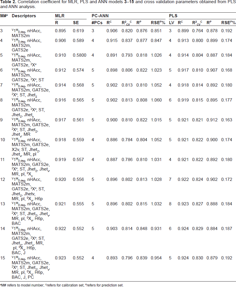
M# refers to model number;

refers for calibration set;

refers for prediction set.

Figure 1

Correlation of R²_CV with MLR model number.

The regression equation for models 4 is:

\begin{array}{l} \log BCF & = & - 18.551 (\pm 1.508) + 1.681 {(\pm 0.075)}^{V} 1^{M}_{D,deg} \\ - 0.535 (\pm 0.030) nHAcc + 16.806 \\ (\pm 1.561) MATS 2 m \\ - 0.417 (\pm 0.084) GATS 2 e \end{array}

(2)

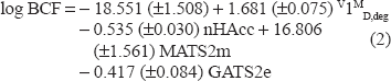
Eq. (2) shows that log BCF can be modeled by 2D autocorrelation descriptors (MATS2 m and GATS2e), the information indices descriptors (_V1^M_{D, deg}) and the functional group descriptor (nHAccc). 2D autocorrekation descriptors are molecular descriptors calculated from molecular graph by summing the products of atom weights of the terminal atoms of all the paths of the considered path length (the lag). 2D autocorrelations by Moran (MATS) and Geary (GATS) algorithms are calculated from lag 1 to lag 8 for 4 different weighting schemes. The information indices descriptors are molecular descriptors calculated as information content of molecules, based on the calculation of equivalence classes from the molecular graph. Eq. (2) shows that the most significant descriptor is the Moran autocorrelation of a topological structure -lag2/weighted by atomic mass (MATS2 m) which is among the 2D autocorrelation descriptors. Furthermore, eq. (2) shows that log BCF increases with increasing MATS2M and _V1^M_{D, deg} and decreases with increasing Geary autocorrelation -lag2/weighted by atomic Sanderson electronegativities (GATS2e) as well as the number of acceptor atoms for H-bonds (nHAcc) values.

Nevertheless, the number of descriptors is small according to the rule of the thumb suggested by Tute.³³ Partial least squares (PLS) and artificial neural networks algorithm (ANN) were used for further investigation of the linear and nonlinear relationships in the obtained regression models.

PC-ANN

The inputs of the ANN were the subset of the descriptors used in different MLR models (Table 2 and S1 in the supplementary material). The correlation data matrix for these descriptors is represented in supplementary material (Table S2). As it is observed, some descriptors represent high degree of collinearity. Collinear descriptors add redundancy to the input data matrix and therefore the performances of the models obtained by using these descriptors will be degraded. Therefore, we used principal components as the inputs of ANN instead of the original descriptors.

Firstly, PCA was used to classify the molecules into training, validation and prediction sets. Performing PCA overall the data set of 229 compounds and 24 descriptors and plotting the first and second principal, shows that compounds 179 and 181 are outliers, see Figure 2. In other words, molecules 179 and 181 behave differently from other molecules with respect to both molecular structure (descriptors) and the logarithm of BCF (log BCF). Therefore, these molecules were not used in the future analysis. According to the pattern of the distribution of the data in factor spaces (Fig. 2) the training, validation and prediction molecules were selected homogenously, so that molecules in different zones of Figure 2 included to all three subsets. After removing the outliers and subjecting the data for the remaining 227 compounds to the preliminary treatment mentioned above, the classified data was used as an input for the ANN.

Figure 2

Correlation of 1st principal component with 2nd principal component for the factor spaces of the descriptors and their BCF.

In this study, a three-layered feed-forward ANN model with back-propagation learning algorithm³⁴ was employed. At the first, the nonlinear relationship between the subset of descriptors selected by step-wise selection-based MLR (Table 2) and log BCF was preceded by PC-ANN models with similar structure. The number of hidden layer's nodes was set 7 for all models and the number of nodes in the input layer was the number of PCs extracted for each subset of descriptors. The results of PC-ANN modeling for MLR models number 3-15 are given in Table 2. This table shows that models 4 and 14 have almost the highest correlation coefficient for the external test set (0.877 and 0.848, respectively) which indicates a high predictive power. The training set correlation coefficients for models 4 and 14 are 0.915 and 0.903, respectively. The R²_CV values for model 4 is 0.837 and the correlation coefficient of prediction is 0.877, which means that the four PCs selected by eigenvalue ranking procedure can explain at least 83.7% and 76.5% variance in log BCF for the calibration and prediction, respectively. Model 14 has a lower R²_CV values (0.814) and correlation coefficient of prediction (R^p = 0.848) than model 4 which models 4 PCs while model 14 models 5 PCs. This suggests that the variables in model 4 are not so strictly correlated between themselves (4 variables represents by 4 PCs) and the network probably would not lose its performance due to collinearity while the variables in model 14 (14 variables) are correlated, they were represented by only 5 PCs.

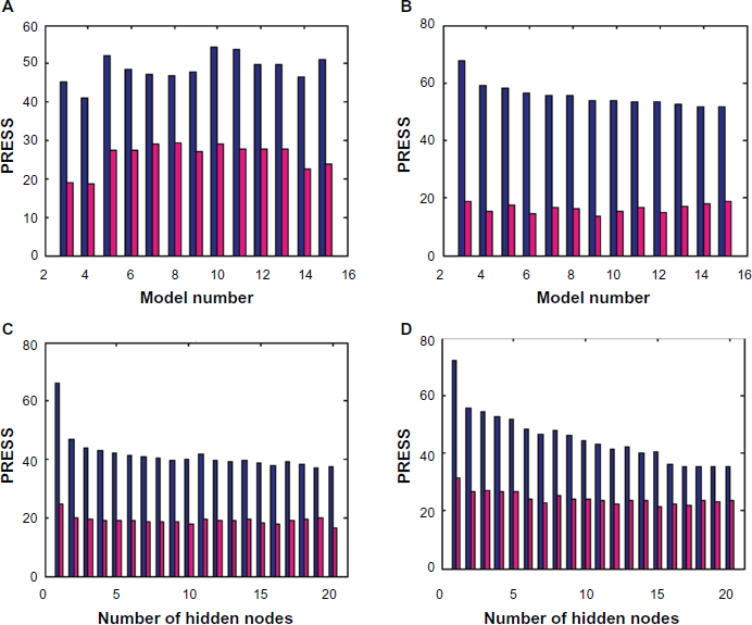
Figure (3a) shows plots of predictive residual sum of squares (PRESS) against regression models number 3 -15 for training and test sets obtained from ANN analysis. As it is seen, the values of PRESS for ANN models 4 and 14 are the minima for training and test sets at the same time which make each of them a good candidate for performing feature analysis on. Hence, the number of hidden nodes for models 4 and 14 was optimized and compared.

Figure 3

A) correlation of PRESS with ANN models (3-15). B) correlation of PRESS with PLS models (3-15). C) correlation of PRESS with different numbers of hidden nodes for ANN model 4. D) correlation of PRESS with different numbers of hidden nodes for ANN model 14.

In order to optimize the performance of the ANN models 4 and 14, we trained the ANN using different number of hidden nodes starting from 1 hidden node to 20 hidden nodes. Figure (3c) shows plots of PRESS against number of hidden nodes for training and test sets for ANN model 4. Although the minima on PRESS curves for this model occurs when using 19 and 20 hidden nodes, such large number of hidden nodes can lead to overfitted models.³⁵ Therefore, we will consider the models with the lower number of hidden nodes (10 hidden nodes, in this case). The PRESS values for the external test set are mainly lower than that for the training set for all models.

The results for the ANN optimization for model 4 are shown in Table S3. Using 19 or 20 hidden nodes gives comparable network performance to that obtained when using 10 hidden nodes. Although the former models have better statistical parameters than those obtained when using 10 hidden nodes, the model obtained using 10 hidden nodes was chosen as the optimal one to avoid the risk of overfitting that may be associated with the use of large number of hidden nodes. Using 10 hidden nodes, we obtained a high correlation coefficient for the training set (0.918) and for the prediction set (0.882). This model has a high R² value for the cross-validation (0.841) and low prediction error (RSE^P% = 0.824%).

Figure (3d) shows plots of PRESS against number of hidden nodes for training and test sets for ANN model 14. The results for the ANN optimization for model 14 are shown in Table S3. This table shows that the minimum on the PRESS curves occurs when using 16-20 hidden nodes. Following the same argument used for model 4, we consider the model with the next lower PRESS value which is in this case 14. For this model, we obtained a relatively high correlation coefficient for both the training (0.917) and the prediction sets (0.845). This model has a high R² value for the cross-validation (0.840) and an RSE^P% value of (0.946%). From a statistical point of view, models 4 and 14 (obtained using 10 and 14 hidden nodes, respectively) are similar. Since large numbers of hidden nodes often draws the attention to overfitting risk,³⁵ model 4 obtained using 10 hidden nodes is preferred over model 14 that is obrained using 14 hidden nodes. The relative standard error of prediction (RSE^P%) is an important parameter for the evaluation of the predictive ability of a multivariate calibration model. RSE^P% is calculated according to eq. (3)

R S E^{P} % = 100 \times \sqrt{\frac{Σ {(\log B C F_{p r e d i c t e d} - \log B C F_{o b s e r v e d})}^{2}}{Σ {(\log B C F_{o b s e r v e d})}^{2}}}

(3)

Model 4 with 10 hidden nodes gives lower RSE^P% (0.824%) than that for model 14 with 14 hidden nodes (0.946%). For deciding on the best model is normally performed by using cross-validation, based on determination of minimum prediction error,³⁶ thus the choice for model 4 with 10 hidden nodes as optimal one is confirmed.

Table S4 in the supplementary material shows the results for randomization test that was performed to investigate the probability of chance correlation for model 4 with 10 hidden nodes in the network. The proposed models were also checked for reliability by permutation testing (Y-scrambling). The results of this procedure (Table S4 in the supplementary material) show that all models have low correlation coefficients and PRESS values. This indicates that model 4, obtained using 10 hidden nodes, has low susceptibility towards chance correlation and gives direct evidence that the proposed models are well founded. Figure 4 demonstrates regression between observed and predicted log BCF as well as their residuals for this model.

Figure 4

Correlation of the predicted log BCF against observed one as well as their residues for A) training set. B) validation set. C) external test set of model 4 obtained by PC-ANN analysis using 10 hidden nodes.

PLS

PLS analysis with cross validation was carried out for advance investigation of the linear relationships of the obtained regression models. Model validation was achieved through leave-one-out cross-validation (LOO CV) and external validation (for a test set), and the predictive ability was statistically evaluated through the root mean square errors of calibration and validation. The calibration and prediction qualities were quantified with the correlation coefficients for the training and test sets as well as the R²_CV (leave one out cross-validation on training set), select the LV when the R²_CV has a high number, or determine it by computing the prediction error sum of squares (PRESS) for cross- validated models which is a standard index to measure the accuracy of a modeling method based on the cross-validation technique.

The cross-validation method employed was to eliminate only one sample at a time and then PLS calibrate the remaining standard descriptor. By using this calibration, the log BCF of the sample left out was predicted. This process was repeated until each standard had been left out once. Figure (3b) shows the associated PRESS of the training and test sets for each model. Table 2 shows that the minimum prediction error (0.163%) occurs for model ⁹. The cross validation coefficient of determination for this model is high (0.821).

This model has the lowest PRESS values for the training and test sets at the same time. While other models have higher R²_CV values than this model, they also have higher prediction errors. Accordingly, model 9 was the best model according to PLS analysis. This model has a regression coefficient of 0.921 and 0.912 for the training and tests sets, respectively.

(Table S5) in the supplementary material shows regression and cross validation parameters for randomization test that is performed to investigate the probability of chance correlation for models 3-15 using PLS analysis. This table shows that the proposed optimal PLS model (model 9) is superior to that obtained by chance. Figure 5 shows regression between observed and predicted log BCF as well as their residuals for training and test sets of model 9 using PLS analysis.

Figure 5

Correlation of the predicted log BCF against observed one as well as their residues for A) training set. B) external test set of model 9 obtained by PLS analysis.

This model contains the following nine descriptors: ^V1^M_{D, deg,} nHAcc, MATS2m, GATS2e, ²X^v, ST, Jhet_Z, Jhet_v, MR (see appendix) which are represented by 5 LV's.

The following conditions proposed by Golbraikh and Tropsha³⁷ were applied to conclude that the QSAR model has acceptable prediction power if:

(1)

Q² (R²_CV) > 0.5

(2)

R² > 0.6

(3)

(R² - R²₀)/R² < 0.1 and 0.85 < k < 1.15

(R²-R′²₀)/R² < 0.1 and 0.85 < k′ < 1.15

where R²₀ and R′²₀ are the coefficients of determination characterizing linear regression with Y-intercept set at zero, the first associated with observed vs. predicted values, the second related to predicted vs. observed values; k and k’ are the slopes of the regression lines forced through zero, relating observed vs. predicted and predicted vs. observed values. Alternatively, the parameter R²_m, where R²_m = R^2* (1-(R²-R²₀))^1/2, can be used.³⁸ This parameter penalizes a model for large differences between observed and predicted values, was also calculated. R²_m should be larger than 0.5 for a good external prediction, which is the case for model 4 from the ANN analysis (R²_m = 0.754) and model 9 from the PLS analysis (R²_m = 0.756). If a model shows good statistical performance for all these criteria, on both the training and the test sets, its reliability and robustness are high.

Comparing the linear (PLS) and nonlinear (PC-ANN) models shows that nonlinear relations improved the models over linear ones. Table 2 shows that compared with PLS and ANN results, MLR underestimate the regression coefficient values for small number of variables. Both ANN and MLR results show that Model 4 is the optimal model to predict the BCF values for the set of compounds in this study. However, PLS analysis improves the statistics compared with ANN and MLR. It gives models with higher correlation coefficients and R²_CV values in addition to lower prediction errors. PLS analysis suggests that the optimal model is model 9. Taking into account the complexity of the neural network based models; PLS based models are better to describe the QSPR of the BCF for the data set in this investigation. The descriptors used in these models depend on the volume, connectivity, molar refractivity, surface tension and the presence of atoms accepting H-bonds.

In summary, this study utilizes theoretical molecular descriptors to estimate BCF directly from the structure of the chemical. The most important molecular descriptors to model the BCF are topological (mainly 2d autocorrelation descriptors), geometrical (mainly encoding molecular size) and generally related to chemicals’ dimensions, polarizability, surface tension, molar ref-reactivity and number of acceptor atoms for H-bonds.

Comparison with previous studies

Table 3 summarizes the results obtained in the present study as well as other QSPR studies performed on the BCF. Zhao et al¹⁴ performed a QSPR study on a large set of 473 compounds that was created with ISIS BASE 2.5 SP2. Wang et al³⁹ obtained a QSAR model by adopting topological properties and flexibility of chemicals to predict the BCF. Gramatica and Papa^16,17 have performed QSAR study on the same set of non-ionic organic compounds using GA and MLR analysis without verifying the data. Fatemi et al¹⁸ applied ANN using descriptors selected with GA but did not use PCA in the stepwise pre-selection of variables. Both Gramatica and Papa^16,17 as well as Fatemi et al¹⁸ split the data randomly, while in this contribution the data is split homogenously using the space of PCs. This implies that the training, validation and test sets include the molecules in different zones of the data distribution shown in Figure 2. Chen et al¹⁹ developed a QSAR model for fish BCFs of 8 groups of compounds employing PLS regression, based on LSER theory and theoretical molecular structural descriptors. Their model showed that the molecular size plays a critical role in affecting the bioconcentration of organic pollutants in fish which agrees with the results found in this study where theoretical descriptors were used to develop the model and assist the mechanism interpretation. Nevertheless, the model found in this study has performed external validation in addition to the usage of a validation set of 46 compounds to detect overfitting as implemented in the early stopping method while no such procedure was used in the other studies mentioned above.

Table 3

Comparison between the different QSAR models.^a

Model	Algorithm	n^A	n^T	n^P	R²	R²_CV	R²_{CV, ex}^b	Val. Set^c
Zhao et al	(HM & GA) -RBFNN	473	378	95	0.83	0.79	NR	NR
Gramatica and Papa (2006)	GA-VSS + OLS	84	53	31	0.77	0.73	0.74	NR
Gramatica and Papa (2003)	GA-VSS + OLS	238	179	59	0.8	0.78	0.88	NR
Fatemi et al	GA-ANN	53	44	9	0.88	0.89-92	NR	NR
Wang et al	PLS	238	202	36	0.84	0.83	0.8	NR
Chen et al	PLS	192	122	70	0.87	0.86	0.76	NR
The current model	PC-ANN	227	135	46	0.84	0.84	NR	R
The current model	PLS	227	181	46	0.85	0.82	NR	NR

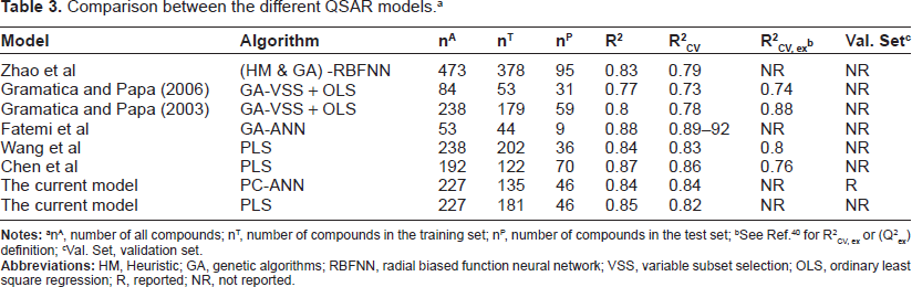
n^A, number of all compounds; n^T, number of compounds in the training set; n^P, number of compounds in the test set;

See Ref.⁴⁰ for R²_{CV ex} or (Q²_ex) definition;

Val. Set, validation set.

Abbreviations: HM, Heuristic; GA, genetic algorithms; RBFNN, radial biased function neural network; VSS, variable subset selection; OLS, ordinary least square regression; R, reported; NR, not reported.

Wang et al obtained coefficients of determination of 0.80 and 0.79 for calibration and cross validation, respectively, while in this study we obtained higher values (0.85 and 0.82). Generally, the calibration and cross validation coefficient of determinations (R² and R²_CV) obtained in this study (ANN model: 0.84 and 0.84/PLS model: 0.85 and 0.82) are higher than those obtained in the other studies shown in Table 3. An exception is for the R² and R²_CV values obtained by Fatemi et al (0.88 and 0.89-0.92) and Chen et al (0.87 and 0.86). However, in this study, we used a larger number of compounds which implies that the results obtained in this study are more general than those obtained by Fatemi et al and Chen et al.

Conclusions

A quantitative-structural property relationship analysis has been conducted on BCF (log BCF) for 227 different non-ionic organic compounds by using PLS and the principal component-artificial neural networks modeling methods, with application of eigenvalue ranking factor selection procedure. The PLS gives improved regression models with better prediction ability compared with PC-ANN. Taking into account the complexity of the neural network based models; PLS based models are quite good to describe the QSPR of the BCF for the data set in this investigation. A 0.921 correlation coefficient was obtained using PLS with 5 LV's. The optimal model contains the descriptors ^V1^M_{D, deg}, nHAcc, MATS2m, GATS2e, ²X^v, ST, Jhet_Z, Jhet_v and MR.

Disclosure

This manuscript has been read and approved by all authors. This paper is unique and is not under consideration by any other publication and has not been published elsewhere. The authors and peer reviewers of this paper report no conflicts of interest. The authors confirm that they have permission to reproduce any copyrighted material.

Footnotes

Acknowledgments

Omar Deeb acknowledges Prof. Dr. Jingwen Chen, Key Laboratory of Industrial Ecology and Environmental Engineering (Ministry of Education), School of Environmental Science and Technology, Dalian University of Technology (China) for his valuable suggestions to improve the manuscript. He also acknowledges Dr. Kunal Roy, Drug Theoretics and Cheminformatics Lab, Department of Pharmaceutical Technology, Jadavpur University, Kolkata (India) for his suggestions concerning validation of the proposed models.

References

Mackay

D.A.

Fraser, Bioaccumulation of persistent Organic Chemicals: mechanisms and Models. Environmental Pollution. 2000; 110: 375–91.

Hodgeson

, Levi

P.E.

Introduction to Biochemical Toxicology, (Appleton and Lange, Norwalk, CT, USA, 1994).

Neely

B.W.

, Branson

D.R.

, Blau

G.E.

Partition Coefficient to Measure Bio-concentration Potential of Organic Chemicals in Fish. Environ Sci Technol. 1974; 8: 1113–5.

Kanazawa

Measurement of the BCFs of Pesticides by Freshwater Fish and their Correlation with Physicochemical Properties or Acute Toxicities. Pestic Sci. 1981; 12: 417–24.

Mackay

Correlation of BCFs. Environ Sci Technol. 1982; 16: 274–8.

Veith

G.D.

, Kosian

Estimating Bioconcentration Potential from Octanol/Water Partition Coefficients, in: Mackay

. editor, Physical Behaviour of PCBs in the Great Lakes, pp. 269 (Ann Arbor Science Pub., USA, 1983).

Isnard

, Lambert

Estimating BCFs from Octanol-Water Partition Coefficient and Aqueous Solubility. Chemosphere. 1988; 17: 21–34.

Schuurmann

, Klein

Advances in Bioconcentration Prediction. Chemosphere. 1988; 17: 1551–74.

Dimitrov

S.V.

, Mekenyan

O.G.

, Walker

J.D.

Non-Linear Modeling of Bioconcentration Using Partition Coefficients for Narcotic Chemicals. SAR QSAR Environ Res. 2002; 13: 177–84.

10.

Bintein

, Devillers

, Karchern

Nonlinear Dependence of Fish Bioconcentration on n-Octanol/Water Partition Coefficient. SAR QSAR Environ Res. 1993; 1: 29–39.

11.

Kubinyi

Nonlinear Dependence of Biological activity on Hydrophobic Character. J Med Chem. 1977; 20: 625–9.

12.

Nendza

QSAR of Bioconcentration: Validity Assessment of log Pow/ logBCF Correlations, in: Nagel

, Loskill

editor, Bioaccumulation in Aquatic Systems, (VCH, Weinheim, 1991) p. 34–66.

13.

Connell

D.W.

, Hawker

D.W.

Use of Polynomial Expression to describe the Bioconcentration of Hydrophobic Chemicals by Fish. Environ Safety. 1988; 16: 242–57.

14.

Zhao

, Boriani

, Chana

, Roncagliono

, Benfenati

A new hybrid system of QSAR models for predicting BCFs (BCF). Chemosphere. 2008; 73: 1701–7.

15.

, Tao

, Hu

, Dawson

R.W.

Estimation of BCFs of nonionic organic compounds in fish by molecular connectivity indices and polarity correction factors. Chemosphere. 2000; 41: 1675–88.

16.

Gramatica

, Papa

QSAR modelling of BCF by the oretical molecular descriptors. QSAR Comb Sci. 2003; 22: 374–85.

17.

Gramatica

, Papa

, Dearden

J.C.

Linear QSAR regression models for the prediction of BCFs by physicochemical properties and structural theoretical molecular descriptors. Chemosphere. 2007; 67: 351–8.

18.

Fatemi

M.H.

, Jalai-Heravi

, Konuze

Prediction of BCF using genetic algorithm and artificial neural network. Anal Chim Acta. 2003; 486: 101–8.

19.

Qin

, Chen

J.W.

, Wang

. Development and assessment of quantitative structure activity relationship models for BCFs of organic pollutants. Chin Sci Bull. 2009; 54: 628–34.

20.

Chen

J.W.

, Li

X.H.

, Yu

H.Y.

. Progress and perspectives of quantitative structure-activity relationships used for ecological risk assessment of toxic organic compounds. Sci China Ser B-Chem. 2008; 51: 593–606.

21.

Chen

J.W.

, Harner

, Ding

G.H.

. Universal predictive models on octanol-air partition coefficients at different temperatures for persistent organic pollutants. Environ Toxico Chem. 2004; 23: 2309–17.

22.

Khadikar

P.V.

, Singh

, Mandaloi

, Joshi

, Bajaj

A.V.

QSAR study on BCF (BCF) of polyhaloginated biphenyls using PI index. Bioorg Med Chem. 2003; 11: 5045–50.

23.

Todeschini

Milano Chemometrics and QSAR Group, http://www.disat.unimib.it/chm.

24.

Chaterjee

, Hadi

A.S.

, Price

Regression Analysis by Examples (3rd ed), (Wiley, New York, 2000).

25.

Gemperline

P.J.

, Long

J.R.V.

, Gregoriou

Gregoriou, Nonlinear multivariate calibration using principal components regression and artificial neural networks. Anal Chem. 1991; 63: 2313–23.

26.

Hemmateenejad

, Shamsipur

Quantitative Structure—Electrochemistry Relationship Study of Some Organic Compounds Using PC-ANN and PCR. Internet Electron J Mol Des. 2004; 4: 316–34.

27.

Hemmateenejad

, Safarpour

, Miri

, Nesari

Toward an Optimal Procedure for PC-ANN Model Building: Prediction of the Carcinogenic Activity of a Large Set of Drugs. J Chem Inf Model. 2005; 45: 190–9.

28.

Deeb

, Hemmateenejad

ANN-QSAR Model of Drug-binding to Human Serum Albumin. Chem Biol Drug Des. 2007; 70: 19–29.

29.

Deeb

, Goodarzi

Predicting the solubility of pesticide compounds in water using QSPR methods. Mol Phys. 2010; 108: 181–92.

30.

Deeb

, Hemmateenejad

, Jaber

, Garduno-Juarez

, Miri

Effects of electronic and physicochemical parameters on the carcinogenic activity of some sulfa drugs using QSAR analysis based on genetic-MLR and genetic-PLS. Chemosphere. 2007; 67L: 2122–30.

31.

Goodarzi

, Freitas

M.P.

Predicting Boiling Points of Aliphatic Alcohols through Multivariate Image Analysis Applied to Quantitative Structure—Property Relationships. J Phys Chem A. 2008; 112: 11263–5.

32.

Deeb

, Youssef

, Hemmateenejad

QSAR of Novel Hydroxyphenylu-reas as Antioxidant Agents. QSAR Comb Sci. 2007; 27: 417–24.

33.

Tute

M.S.

History and Objectives of Quantitative Drug Design in Advances in Research

Drug

, Harter

N.J.

, Simmord

A.B.

, editors. Vol. 6, (Academic Press, London, 1971) p. 1.

34.

Rumelhart

D.E.

, Hinton

G.E.

, Williams

R.J.

Learning representations by back-propagating errors. Nature. 1986; 323: 533–6.

35.

Derks

EPPA

, Buydens

L.M.C.

Aspects of network training and validation on noisy data Part 1. Training aspects. Chemom Intell Lab Syst. 1998; 41: 171–84.

36.

Martens

, Naes

Multivariate Calibration. John Wiley, Chichester. 1989.

37.

Golbraikh

, Tropsha

Beware of q2!. J Mol Graph Model. 2002; 20: 269–76.

38.

Roy

, Roy

Comparative chemometric modeling of cytochrome 3 A4 inhibitory activity of structurally diverse compounds using stepwise MLR, FA-MLR, PLS, GFA, G/PLS and ANN techniques. Eur J Med Chem. 2009; 44: 2913–22.

39.

Wang

, Lib

, Dinga

, Jianga

, Changa

Estimation of BCFs using molecular electro-topological state and flexibility. SAR QSAR Environ Res. 2008; 19: 375–95.

40.

Schüürmann

, Ebert

, Chen

J.W.

, Wang

, Kühne

External Validation and Prediction Employing the Predictive Squared Correlation Coefficient Test Set Activity Mean vs Training Set Activity Mean. J Chem Inf Model. 2008; 48: 2140–5.

QSPR Modeling of Bioconcentration Factors of Nonionic Organic Compounds

Abstract

Keywords

Introduction

Experimental

Software

Chemical data and descriptors

MLR analysis

PC-ANN

Partial least squares (PLS) analysis

Results and Discussion

MLR analysis

PC-ANN

PLS

Comparison with previous studies

Conclusions

Disclosure

Footnotes

Acknowledgments

References