Promoter Sequences Prediction Using Relational Association Rule Mining

Abstract

In this paper we are approaching, from a computational perspective, the problem of promoter sequences prediction, an important problem within the field of bioinformatics. As the conditions for a DNA sequence to function as a promoter are not known, machine learning based classification models are still developed to approach the problem of promoter identification in the DNA. We are proposing a classification model based on relational association rules mining. Relational association rules are a particular type of association rules and describe numerical orderings between attributes that commonly occur over a data set. Our classifier is based on the discovery of relational association rules for predicting if a DNA sequence contains or not a promoter region. An experimental evaluation of the proposed model and comparison with similar existing approaches is provided. The obtained results show that our classifier overperforms the existing techniques for identifying promoter sequences, confirming the potential of our proposal.

Introduction

Association rule mining means searching attribute-value conditions that occur frequently together in a data set.^1,2 Ordinal association rules ³ are a particular type of association rules. Given a set of records described by a set of attributes, the ordinal association rules specify ordinal relationships between record attributes that hold for a certain percentage of the records. However, in real world data sets, attributes with different domains and relationships between them, other than ordinal, exist. In such situations, ordinal association rules are not powerful enough to describe data regularities. Consequently, we have introduced relational association rules ⁴ in order to be able to capture various kinds of relationships between record attributes. Relational association rule mining can be used in solving problems from a variety of domains, such as: Data Cleaning, Natural Language Processing, Databases, HealthCare.

In this paper, based on the idea of discovering relational association rules within a data set, we propose a classification model for the problem of promoter sequences prediction. The problem of predicting if a DNA sequence contains or not a promoter region is an important problem in bioinformatics, mainly because determining the promoter region in the DNA is a significant step in the process of detecting genes. This classification problem was already approached both in the biological and computer science literature, offering this way the opportunity to relate our proposal to similar existing ones. We have to emphasize that the problem mentioned above is approached from a computational perspective, without looking into deep biological insights of it. We are focusing on developing a machine learning based computational model that will be powerful enough (as shown in the experimental section) to capture aspects that are relevant in distinguishing between DNA sequences that contain or not a promoter region. In building our classifier, we try to interpret DNA sequences both by their biological and chemical properties and to exploit the benefit of data mining techniques to uncover hidden patterns in data.

The results obtained by evaluating the classification model proposed in this paper confirm that applying relational association rule mining for promoter sequences recognition is promising and indicate the potential of our proposal. Moreover, the use of relational association rules in classifying promoter sequences, proposed in this paper, is a novel approach.

Motivation

Relational association rules were introduced as an extension to association rules, in order to be able to discover various kinds of relations or correlations that exist between data in large data sets. Classical association rules discard any quantitative information that may exist between record attributes in data sets, but many times this type of information can give valuable insights into the problem at hand. The record attributes may be in an ordinal relationship, if the domains of the attributes are similar or comparable. Otherwise, when the attributes do not have commensurable values, more general relations are needed, ones that are powerful enough to capture different interesting relationships between data. Therefore, the extension of classical association rules towards ordinal and more general, relational association rules allows the uncovering of much stronger rules that consequently achieve superior data mining, or classification.

For example, considering a data set composed of many DNA sequences, which represent the records and where the record attributes are the nucleotide bases, significant information can be extracted from the chemical and physical properties of the nucleotides. Therefore, relations between attributes could be given by such characteristics. Measurable, comparable properties, like molar mass, density or acidity may be easily used to generate ordinal association rules. However, other properties, which cannot be quantified, like the class the compound belongs to in a certain thesaurus or classification, or the biomo-lecular interactions it can perform could also have an impact in mining or classification. Consequently, there appears the need to define different types of relations in order to take into consideration all kinds of relevant properties.

In a relational association rule mining or classification task, the objective is to find several relationships between the attributes that tend to hold over a large percentage of records. In a binary classification problem, if attribute A is in relation with attribute B for a great number of positive instances, then a record in which attribute A is not in relation with attribute B may be a negative instance. It may not mean very much if only one rule including B is not fulfilled, but if many such rules are broken, then the likelihood that the instance in question belongs to the negative class increases.

We have started from the intuition that in the problem of deciding if a DNA sequence contains or not promoter regions, relationships between the nucleotides that form the DNA sequence may be relevant. These relationships may express quantitative information that may exist in a DNA sequence, and it is likely that this type of relationships could significantly influence the classification task.

Promoter Sequences Prediction

In this section we aim at presenting the problem of promoter sequences prediction and its relevance, as well as existing machine learning based approaches for solving the considered problem.

The problem statement and relevance

Proteins are one of the most important classes of biological molecules, being the carriers of the message contained in the DNA. There are two processes that are involved in the synthesis of proteins, the first of these being transcription. During transcription, a single stranded RNA molecule, called messenger RNA is synthesized (using the complementarity of the bases) from one of the strands of DNA corresponding to a gene (a gene is a segment of the DNA that codes for a type of protein). This process begins with the binding of an enzyme called RNA polymerase to a certain location on the DNA molecule. This exact site, that determines which of the two strands of DNA will be transcript and in which direction, is recognized by the RNA polymerase due to the existence of certain regions of DNA placed near the beginning of a gene, regions called promoters.

Because determining the promoter region in the DNA is an important step in the process of detecting genes, the problem of promoter identification is of major importance within bioinformatics. As the conditions for a DNA sequence to function as a promoter are not known, Machine Learning methods are suitable to approach this problem because they can learn useful descriptions of concepts when given only instances–-DNA sequences that are assumed to contain underlying but unknown patterns of base pairs. ⁵

In the context of Supervised Machine Learning, the identification of promoters can be stated as follows: given two sets of DNA sequences of fixed length, one containing sequences with known promoter regions and the other one containing sequences without the presence of this signal, generate a classifier able to predict whether a fixed length “window” of a DNA sequence contains or not promoter regions. ⁶

Related work

Several machine learning approaches have been applied in order to recognize biological signals (such as promoters) that enable the transcription process.

A hybrid learning system, that combines explanation based learning and empirical learning was proposed by Towell et al. ⁷ The Knowledge-Based Artificial Neural Networks (KBANN) system uses a knowledge base of approximately correct, domain-specific rules and translates them into an Artificial Neural Network, whose structure and initial weights correspond to parts of the knowledge base. In order to test this algorithm, the authors investigate the promoter identification problem. They developed a data set of 106 E. coli DNA subsequences (53 of which contained promoters, thus representing positive examples and 53 being negative examples), each sequence containing 57 nucleotides. Results obtained by artificial neural networks created by KBANN were compared to those obtained by standard back propagation networks, classification trees and nearest neighbor methods and the proposed method proved to be superior to the other three learning algorithms.

Pedersen and Engelbrecht ⁸ present a new method that uses a neural network in order to discover signals that imply the existence of promoters in regions of DNA. The authors used a classic version of feedforward artificial neural network, with an input layer (that contained the DNA sequence, encoded into a binary string), one hidden layer (with two or three neurons) and an output layer consisting of only one neuron. The experiments were made on a data set of 167 E. coli DNA sequences. For each of the 167 sequences, the training and test input values for the networks were constructed by sliding a window over the entire sequence in order to obtain positive and negative examples (of 65 nucleotides). In addition to this type of construction, the new method the authors introduce feeds the network with the same windows, but which contain a hole (of length 7 base pairs). This way they detect the local regions with significant information by searching for positions of the hole that causes the learning ability of the network to be partially destroyed.

A new approach for predicting promoters from a data set of 2111 samples from 4 species (among which Homo Sapiens and E. coli) is proposed by Tatavarthi et al. ⁹ It is based on the machine learning algorithm called Grey Relational Analysis (GRA). In a GRA approach, a system that has no information is defined as black, one that is full of information is called white, while a system that has incomplete or undetermined information is defined as grey. Thus, a grey element or relation in such a system represents an element or a relation with incomplete information. Using the basic definitions of a GRA system, the grey relational grade of a test sequence is computed, with respect to a certain number of comparative sequences (from the data set). Then, this grade is used to measure the relationship between the test sequence data and comparative sequences data.

Multiple Support Vector Machine (SVM) approaches for the problem of promoter recognition have been proposed, one of these being presented by Kasabov and Pang. ¹⁰ More specifically, the authors introduce a novel Transductive Support Vector Machine (TSVM), which develops a model for every new input vector, based on specific training examples and then uses the model to predict the output only for the specific input vector. This technique differs from the traditional inductive SVMs, that build a general model using the training data and then apply the obtained model on the entire test data. Both the inductive and transductive SVMs were trained and tested using a data set of 793 different vertebrate promoter sequences of length 250 base pairs and another 1200 human DNA sequences, of the same length. The TSVM has proven to outperform the inductive SVM on the task of promoter recognition.

Although, to our knowledge, association rules have not been used for the specific task of detecting promoters, there are some approaches that use association rules mining in the context of gene expression and signal recognition in promoter sequences. Icev et al ¹¹ determine the expression patterns of certain genes by building a new type of association rules–-distance-based association rules. These rules are based on short sequences of DNA, called motifs, that are contained in promoters and to which certain gene regulatory proteins may bind. Shibayama et al ¹² obtained successful results when extracting simple association rules in order to find signals in mammalian promoter sequences.

Relational Association Rules. Background

In order to be able to capture various kinds of relationships between record attributes, the definition of ordinal association rules^3,13 was extended towards relational association rules. ⁴

In the following we will briefly review the concept of relational association rules, as well as the mechanism for identifying the relevant relational association rules that hold within a data set.

Let R = {r₁, r₂, …, r _n } be a set of instances (entities or records in the relational model), where each instance is characterized by a list of m attributes, (a₁, …, a _m ). We denote by ϕ(r _j , a _i ) the value of attribute a _i for the instance r _j . Each attribute a _i takes values from a domain D _i , which contains the empty value. Between two domains D _i and D _j relations can be defined (not necessarily ordinal relations), such as: less or equal (≤), equal (=), greater or equal (≥), etc. We denote by M the set of all possible relations that can be defined on D _i × D _j .

Definition 1: ⁴ A relational association rule is an expression (a _{i 1} , a _{i 2} , a _{i 3} , …, a _{i l} ) ⇒ (a _{i 1} μ₁ a _{i 2} μ₂ a _{i 3} … μ_l-1 a _{i l} ) where {a _{i 1} , a _{i 2} , a _{i 3} , …, a _{i l} } ⊆ A = {a _{i 1} …, a _{i m} }, a _{i j} ≠ a _{i k} , j, k = 1 … l, j ≠ k and μ _i ∈ M is a relation over D _{i j} × D_{j + 1 j} , D _{i j} is the domain of the attribute a _{i j} . If:

• a)

a _{i 1} , a _{i 2} , a _{i 3} , …, a _{i l} occur together (are non-empty) in s% of the n instances, then we call s the support of the rule, and

b)

we denote by R' ⊆ R the set of instances where a _{i 1} , a _{i 2} , a _{i 3} , …, a _{i l} occur together and ϕ (r', a _{i 1} ) μ₁ μ₁ ϕ(r', a _{i 2} ) μ₂ ϕ(r' a _{i 3} ) … μ_l-1 ϕ(r, a _{i l} ) is true for each instance r' from R';then we call c = |R'|/|R| the confidence of the rule.

We call the length of a relational association rule the number of attributes in the rule. The length of a relational association rule can be at most equal to the number m of the attributes describing the data.

The users usually need to uncover interesting relational association rules that hold in a data set; they are interested in relational rules which hold in a minimum number of instances, that is rules with support at least s _min , and confidence at least c _min (s _min and c _min are user-provided thresholds).

Definition 2: ⁴ We call a relational association rule in R interesting if its support s is greater than or equal to a user specified minimum support, s _min , and its confidence c is greater than or equal to a user-specified minimum confidence, c _min .

An A-Priori ¹⁴ like algorithm, called DOAR (Discovery of Ordinal Association Rules) ¹³ , was introduced in order to efficiently find all ordinal association rules (i.e., relational association rules in which the relations are ordinal) of any length, that hold over a data set. The mechanism of discovering interesting ordinal association rules in a data set will be extended in our approach towards identifying relational association rules.

In the following a brief description of the idea of discovering interesting ordinal association rules will be given. ¹³ This algorithm identifies ordinal association rules using an iterative process that consists in length-level generation of candidate rules, followed by the verification of the candidates for minimum support and confidence compliance. DOAR performs multiple passes over the data set R. In the first pass, it calculates the support and confidence of the 2-length rules and determines which of them are interesting, i.e., verify minimum support and confidence requirement. Every subsequent pass over the data consists of two phases. The first phase starts with a seed set of (k-l)-length (k ≥ 3) interesting rules, found in the previous pass. This set is used to generate new possible k-length interesting rules, called candidate rules. The candidate generation process is a key element of the DOAR algorithm. During the second phase, a scan over the R data is performed in order to compute the actual support and confidence of the candidate rules. At the end of this step, the algorithm keeps the rules that are deemed interesting (have minimum support and satisfy the confidence requirements), which will be used in the next iteration. The process stops when no new interesting rules were found in the latest iteration.

The DOAR algorithm significantly prunes the exponential search space of all possible interesting ordinal association rules, due to the candidate generation technique. The candidate generation restricts the search to those regions of the search space where it is possible that interesting rules exist, pruning out all the regions where it is impossible to find any interesting rules. The search space reduction depends on the data being analyzed. The larger the number of interesting rules in the data set is, the larger the size of the candidates sets will be.

DOAR algorithm is proven to be correct and complete and it efficiently explores the search space of the possible rules. ¹³ The DOAR algorithm is extended in our approach towards DRAR algorithm (Discovery of Relational Association Rules) for finding interesting relational association rules, i.e., association rules which are able to capture various kinds of relationships between record attributes.

Our current implementation provides two functionalities:

• •

finds all interesting relational association rules of any length.

•

finds all maximal interesting relational association rules of any length, i.e., if an interesting rule r of a certain length l can be extended with one attribute and it remains interesting (its confidence is greater than the threshold), only the extended rule is kept.

Methodology

In this section we propose a supervised learning technique in order to predict promoter sequences, based on relational association rules mining, called PCRAR (Promoter sequences Classifier using Relational Association Rules).

Although there are some fundamental differences between promoters in eukaryotic and prokaryotic organisms, it was not our goal to design an organism specific system, that would recognize certain classes of promoters or special nucleotide motifs. The classifier was built with the purpose of distinguishing DNA sequences that contain promoters from those that do not. Therefore, our PCRAR classifier is not based on any particular biological mechanisms, its strength consisting in its ability to automatically learn the differences between DNA sequences that include or not promoter regions, when given as input only these sequences and no other extra biological information.

The problem that we are focusing on is a binary classification problem. There are two possible classes, denoted in the following by “+” and “-” By “+” we denote the class corresponding to DNA sequences that contain promoter regions, and the sequences that belong to the “+” class will be referred to as positive instances or promoters. By “-” we denote the class corresponding to DNA sequences that do not contain promoter regions, and the sequences that belong to the “-” class will be referred to as negative instances or non-promoters.

The main idea of our approach is the following. In a supervised learning scenario for predicting promoter sequences, two sets containing positive and negative instances are given. These sets will be used for training the classifier. During training, the DRAR algorithm will be used. Even if this algorithm can be used to discover all the relational rules, of any length, in a data set, we used it to discover only the binary relational association rules, i.e., relational association rules of length two. In our approach, binary rules are sufficient in order to classify a DNA sequence as a promoter or non-promoter. We detect in the training data sets all the interesting binary relational rules (rules between two attributes), with respect to the user-provided support and confidence thresholds). After the training was completed, when a new instance (DNA sequence) has to be classified (as “+” or “-”), we reason as follows. Considering the binary rules discovered during training in the set of positive and negative instances, the probability to assign the instance to the “+” class will be computed. If this probability is greater or equal to 0.5, then the query instance will be classified as a positive instance, otherwise it will be classified as a negative instance.

Let us consider, in the following that we are focusing on DNA sequences having a fixed length. We consider a DNA sequence (instance) as an n-dimensional chain (sequence) S = (s1, s₂, …, s _n ) containing the four letters A, T, G and C, which represent the nucleotides composing the DNA (A-Adenine, T-Thymine, G-Guanine, C-Cytosine). ¹⁵ Consequently, the attribute (feature) set characterizing the instances (DNA sequences) is an n-dimensional list A = (A₁,A₂, …, A _n ), where attribute A _i corresponds to the i-th nucleotide from the DNA sequence. Therefore, each attribute A _i . (∀1 ≤ i ≤ n) has 4 possible values: the characters A, T, G and C.

The process takes place in two phases that reflect the principles of a supervised learning algorithm: training and testing. During the training, a classification model will be built, and during testing, the model built during the training will be applied for classifying an unseen instance. As mentioned above, we consider for training two data sets: DS₊ consisting of positive n-dimensional instances (DNA sequences that contain a promoter region) and DS_– consisting of negative n-dimensional instances (DNA sequences that do not contain a promoter region). These data sets are used in the training step of the PCRAR classifier and a classification model consisting of the discovered relational association rules is built. At the classification time, when a new instance (DNA sequence) S has to be classified, the model learned during the training step will be used for computing the probability that the sequence S is a positive or a negative instance, i.e., it contains or not a promoter region.

For classifying a DNA sequence as containing or not a promoter region, the following steps will be performed:

1. 1)

Relations definition.

2)

Data pre-processing.

3)

Training/building the PCRAR classifier.

4)

Testing/classification.

In the following we will describe this steps.

Relations definition

This step is an important part of the classification process, it deals with defining the relations between the attributes values that will be used in the relational association rule mining process. More exactly, we are focusing on identifying relations between two nucleotides from a DNA sequence (A, T, G or C), relations that would be relevant for deciding if the sequence contains or not a promoter region, and consequently would be useful in the mining process.

The following two steps are performed in order to complete our task.

Step 1: First, we search for several computed chemical and physical properties that may characterize each nucleotide. Most of the properties we used were extracted from PubChem, ¹⁶ which represents three linked databases that provide information about small molecules. We selected the following measurable properties:

1. 1)

Molar mass

2)

Density

3)

Topological Polar Surface Area

4)

Heavy Atom Count

5)

Complexity

6)

Base composition

The last property, base composition, is one of the most fundamental features of a DNA sequence and it refers to the percentages of each of the four different nucleotides, on one strand of DNA. We computed the base composition for each nucleotide, using the complete genome of E. coli K-12, as catalogued in GenBank database. ¹⁷

Consequently, we associate to each nucleotide (attribute value) a list of six numerical codes, representing the values of the six above enumerated properties. As an example, for the first property-molar mass, we have the following values for the four nucleobases (according to PubChem): A (adenine)-135.13, C (cytosine)-111.1, G (guanine)-151.13, T (thymine)-126.11. The associated properties, together with the corresponding normalized values are illustrated in Table 1.

Table 1

Codes representing measurable physical and chemical properties.

Code ID	Property name	A	C	G	T
C1	Molar mass	0.8941	0.7351	1	0.8344
C2	Density	0.7272	0.7045	1	0.5590
C3	Topological Polar surface area	0.8367	0.7016	1	0.6049
C4	Heavy atom count	0.9090	0.7272	1	0.8181
C5	Complexity	0.5644	0.7555	1	0.8666
C6	Base composition	0.9681	1	0.9976	0.9673

As we are focusing in our approach on exploiting relations between the four nucleotides, it can be observed that codes C1 and C4 are equivalent, as the way they rank the four nucleotides is the same. Another equivalence can be observed between codes C2 and C3.

Step 2: The second step is to identify which of the six types of codes associated to the attributes (C1-C6) would be relevant for the classification task. In this direction, a statistical analysis is performed on the training data sets DS₊ and DS_– to determine those codes that provide attributes highly correlated with the target output. We consider the target classification output to be 1 if a DNA sequence contains a promoter region, and 0 otherwise.

To determine the dependencies between attributes and the target output, the Spearman's rank correlation coefficient ¹⁸ is used. A Spearman correlation of 0 between two variables X and Y indicates that there is no tendency for Y to either increase or decrease when X increases. A Spearman correlation of 1 or -1 results when the two variables being compared are monotonically related, even if their relationship is not linear.

Using the Spearman's rank correlation coefficient between attributes and the target output, we reason as follows. For each of the six types of codes associated to the attributes, we compute the average correlation as the average of the absolute values of the correlation coefficients between each attribute (considering the given code as the attribute value) and the target output. Only the codes that provide the highest average correlations to the target output will be further considered in order to define the relations between attributes and to mine the interesting relational association rules. In order to select the relevant codes, firstly, we compute the mean value M of the average correlations between the six codes and the target classification output. Then, we consider that a code is likely to be relevant in the mining process only if its average correlation with the output is above M with at least γ, where γ is a small threshold (e.g., 0.005).

The computational process described above will be illustrated on a practical example in Section Experimental Evaluation, where we introduce the specific dataset used for performing the calculations. The same section will present, in detail, how we determined which of the six types of codes (C1-C6) are relevant for our classification task, without using a priori biological knowledge about the connection between these properties and promoter sequences in the DNA.

Let us consider that following the statistical analysis described above, from the set C = {C₁, C₂, …, C₆} only a subset C' ⊂ C was selected as containing types of codes that are relevant in defining the relational association rule model. Consequently, the relations between two nucleotides will be given as relationships between their corresponding numerical codes. Considering a given type of code c ∈ C', three relations between the nucleotides are defined: =_c, <_c and > _c (e.g., if s₁ and s₂ are two nucleotides then we consider that s₁ <_c s₂ iff c(s₁) < c(s₂); here by c(s) we mean the numerical value (code) associated to the nucleotide s considering the property indicated in Table 1 by the type of code c. As relation = does not depend on a particular type of code c), the final set R of relations considered for the relational association rule mining task is considered as $R=\{=\}\cup {\cup }_{c\in C^{\prime }}\{{<}_c,{>}_c\}$ .

Data pre-processing

After a set C' containing types of codes that are relevant in defining the relational association rule model was identified (Subsection Relations Definition), another statistical analysis is carried out on the training data sets DS₊ and DS_– in order to find a subset of attributes that are correlated with the target output. The statistical analysis on the attributes is performed in order to reduce the dimensionality of the input data, by eliminating attributes which do not influence the output value.

To determine the dependencies between attributes and the target output, the Spearman's rank correlation coefficient is used. The goal of this step is to remove from the attribute set A = (A₁, A₂, …, A _n ) (Section Methodology) those attributes (nucleotides at a certain position, in our example) that have no significant influence on the target output, i.e., are slightly correlated with it (the absolute value of the correlation is below a small positive threshold ε). A slight correlation is indicated by a value that is very close to 0. We mention that the correlations between the attributes and the target classification are computed considering all the types of codes from the set C'.

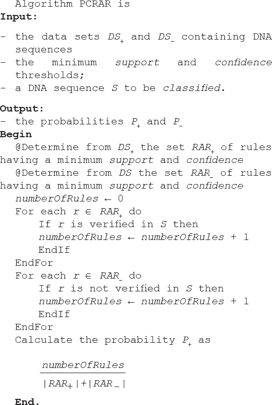
Building the PCRAR classifier

The data sets, pre-processed as indicated in Subsection Data pre-processing, considering the set R of relationships between the attributes domains defined in Subsection Relations Definition, can now be used for building the relational association rule based classification model.

At this step, the interesting relational association rules are discovered in the training data sets. As in an eager ¹⁹ classification task, the classification model consisting of interesting relational association rules discovered in the training data sets will be further used to classify all test instances.

More exactly, the training consists of the following steps:

• •

Determine from DS₊, using the DRAR algorithm, the set RAR₊ of relational association rules having a minimum support and confidence.

•

Determine from DS_–, using the DRAR algorithm, the set RAR_– of binary relational association rules having a minimum support and confidence.

Classification using PCRAR

At the classification stage, after the training was completed and the PCRAR classifier was built, when a new DNA sequence S has to be classified, we calculate the probability P₊ that S contains a promoter region and P_– the probability that S does not contain a promoter region. From a Bayesian learning perspective, it is about determining the most probable classification (+ or -) of a new instance (DNA sequence), given the training data D = DS₊ ∪ DS_–. More exactly, we propose a simple method to compute the conditional probabilities P(+|D) (denoted P₊) and P(-|D) (denoted P_–), but instead of using a bayesian approach (e.g., Bayes theorem) we introduce a method to compute these conditional probabilities considering the sets of interesting relational association rules that were identified in the training data (i.e., RAR₊ and RAR_–). The way we propose to compute P₊ and P_– is simple, the accuracy of these computations being given in fact by the sets RAR₊ and RAR_–. We have started from the intuition that the more relevant the relational association rules detected in the training data, the more precise the probabilities will be. That is why our main focus is toward identifying accurate and significant relations in the training data. This assumption was validated in the experimental part presented in Section Experimental Evaluation. Alternative methods to compute the probabilities P₊ and P_– will be further investigated.

The steps that we propose for computing the conditional probabilities are:

• •

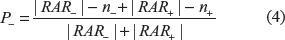
Determine n₊ the number of relational association rules from RAR₊ that are verified in the sequence S. Consequently, the number m₊ of relational association rules from RAR₊ that are not verified in the sequence S is m₊ = |RAR₊| - n₊.

•

Determine n_– the number of relational association rules from RAR_– that are not verified in the sequence S. Consequently, the number m_– of relational association rules from RAR_– that are verified in the sequence S is m_– = |RAR_–| - n_–.

•

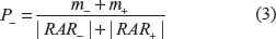
Calculate the probability P₊ to classify an instance as a positive one as $\frac{n_{+}+n_{-}}{\left|RA{R}_{+}|+|RA{R}_{-}\right|}$ . By |A| we have denoted the cardinality of the set A.

If P₊ ≥ P_– then the instance S will be classified as a positive instance, otherwise it will classified as a negative instance.

At the classification stage, we can also compute the probability P_– to classify an instance as a negative one as P_– $P_{-}=\frac{m_{-}+m_{+}}{\left|RA{R}_{-}|+|RA{R}_{+}\right|}$ . However, this step can be skipped as it can be easily proven that the results provided by the PCRAR classifier are logically consistent, meaning that for a given instance S, P₊ + P_– = 1. We give below a lemma which proves that the sum of the probabilities of the two possible outcomes (an instance to be classified as positive or negative) is 1.

Lemma 1: Let P₊ be the probability that a DNA sequence S is a promoter and let P_– be the probability that S is a non-promoter, as reported by the PCRAR classifier. In this case, equality (1) holds:

$$P_{+}+P_{-}=1$$

We prove below Lemma 1.

Proof:

Using the considerations above, we have the following:

$$P_{+}=\frac{n_{+}+n_{-}}{\left|RA{R}_{+}|+|RA{R}_{-}\right|}$$

and

$$P_{-}=\frac{m_{-}+m_{+}}{\left|RA{R}_{-}|+|RA{R}_{+}\right|}$$

It is obvious that n₊ + m₊ = |RAR₊| and n_– + m_– = |RAR_–|.

Consequently, Equation (4) below holds.

$$P_{-}=\frac{\left|RA{R}_{-}\left|-n_{-}+\right|RA{R}_{+}\right|-n_{+}}{\left|RA{R}_{-}|+|RA{R}_{+}\right|}$$

From Equations (2) and (4) it follows that:

$$P_{-}=1-P_{+}$$

So Lemma 1 is proved.

We give next the PCRAR algorithm, the classification technique that was introduced above.

Remark 1: Regarding the classification process, we remark the following:

• •

We remark that in computing the probability P₊ to classify an instance as positive, only the number of rules that are verified/not verified in a data set is considered, without referring to the confidence of the rule. We have started with this simple computation mode, without considering the confidence and support of the rules, because we wanted to have a mathematical support for these computations (see Lemma 1). If the confidence and support of the rules would be considered too, P₊ and P_– would not be probabilities, meaning that Lemma 1 could not be proven.

•

Consequently, considering that a certain rule with a length greater than two is verified if its binary sub rules are verified, it is enough to generate only the binary interesting relational rules. Thus, the training time of PCRAR classifier is significantly reduced, as only binary rules are generated. This fast training is a major advantage of our proposal.

•

If instead of using only the number of relational association rules that are verified/not verified in the training data we would also consider the confidence of the generated rules, it is very likely that rules of any length should be generated, not only binary rules. Further improvements of our approach will investigate this situation.

Experimental Evaluation

In this section we aim at experimentally evaluating our approach for promoter sequences recognition using relational association rules, as well as providing a comparison with other existing similar approaches. The case study used in our experiment, the methodology used, as well as the obtained results are presented in the following subsections.

Data set

The data set we used to test the efficiency of the PCRAR classifier is entitled “E. coli promoter gene sequences (DNA) with associated imperfect domain theory”. This data set was taken from the UCI Repository ²⁰ and contains a set of 106 promoter and non-promoter instances. We have considered this data set in our experimental evaluation, despite the fact that it was built and used in researches before 1990, for two reasons: first, because information about this data set (including its previous usage) are publicly available; and second, as classifiers were already developed and validated on this data set, comparisons of our PCRAR classifier with the models existing in the literature can be conducted.

The task is to recognize promoters in the DNA of a bacterium called Escherichia coli (E. coli). This bacterium is often used as a model organism in microbiology, being one of the first organisms that had their genome sequenced. This data set was developed to the purpose of evaluating a “hybrid” learning algorithm–-KBANN, ⁷ and it has also been studied from a biological perspective by Harley and Reynolds. ²¹

The data set is composed of 106 DNA sequences, each having a length of 57 nucleotides. Half of the 106 sequences represent positive instances, i.e, they contain promoter regions, while the other 53 are negative instances. The positive instances were aligned so that the transcription initiation site for each occurred seven nucleotides from the right edge of the window. For each instance, three types of information are given, in the following order:

1. 1.

“+/-”–-indicating the class (“+” represents the promoters).

2.

The name of the given instance.

3.

The DNA sequence itself, a chain containing the four letters A, T, G and C, which represent the nucleotides composing the DNA (A-Adenine, T-Thymine, G-Guanine, C-Cytosine). ²² The starting position of the sequence is -50, while the ending position is +7 (with respect to the site at which RNA polymerase binds to the DNA sequence).

Past usage of the data set: From a machine learning perspective, the data set was used in order to classify an instance as a promoter (positive instance–-“+”) or non-promoter (negative instance–-“-”).

As indicated above, the data set considered in our experiment, was previously used to evaluate a “hybrid” learning algorithm, named KBANN, ⁷ which used examples to inductively refine preexisting knowledge. The authors of this study indicated that machine learning techniques, like neural networks, ¹⁹ nearest neighbor, ¹⁹ decision tree, ²³ KBANN system performed as well/better than classification based on canonical pattern matching ²⁴ (method used in the biological literature).

For evaluating the performance of the previously mentioned learning algorithms, a cross-validation ²⁵ using a “leave-one-out” methodology was applied and the errors indicated in Table 2 were reported. ⁷ We mention that the error of a classifier indicates the percentage of misclassified instances, i.e, in Table 2 an error of 4/106 indicates 4 misclassified instances from the total of 106 instances.

Table 2

Obtained errors.

System	Error	Comments
KB 7	4/106	A hybrid ML system
BP	8/106	Neural network with one hidden layer
O'Neill 26	12/106	Ad hoc technique from the biological literature
NN	13/106	A nearest-neighbor algorithm (k = 3)
ID3	19/106	Quinlan's decision-tree builder

Case study

In this section we illustrate how the PCRAR classifier introduced in Section Methodology is applied for promoter sequences prediction, using the case study described in Subsection Data set. In the following we detail the steps described in Section Methodology used in order to build the relational association rule based classifier.

Relations definition: As mentioned in Section Methodology, the first stage of our approach consists in defining the relations between the attributes values that will be used in the relational association rule mining process.

Each attribute is, in fact, represented by a nucleotide and, as mentioned in Subsection Relations Definition, each nucleotide may be characterized by a real value, representing a measurable chemical or physical property of the molecule. We used six types of codes, which were enumerated in the above mentioned subsection.

We aim to determine which of the six types of codes associated to the attributes provide high correlations (considering the Spearman's rank correlation coefficient) with the target classification. As we have mentioned in Subsection Relations Definition, we are considering those codes whose average correlation with the output is above the mean value with at least γ. In our current implementation the value of the threshold γ was selected 0.005. Further extensions of our approach will investigate methods to automatically determine, in a supervised learning manner, the value for the threshold γ. As a result of the above analysis, we concluded that the codes identified in Table 1 by C5 (Complexity) and C6 (Base composition), representing the values for Complexity and Base composition produce the highest average correlations to the target output (as the average correlation value for C5 is above the mean with 0.0083 and the average correlation value for C6 is above the mean with 0.0341) and therefore we decided to use a combination of these codes in order to define the relations between attributes and eventually to mine the interesting relational association rules. Figure 1 illustrates the average degree of correlation to the target output of all of the six codes. Considering a particular code, the average correlation is computed as the average of the absolute values of the correlation coefficients between each attribute (considering the given code as the attribute value) and the target output.

Figure 1

Codes correlations.

Consequently, for our case study, as we have presented in Subsection Relations Definition, five possible relations between the nucleotides are considered in the mining process: =,< _C5 , < _C6 , > _C5 and > _C6 .

We observe in Figure 1 that codes C1 and C4, C2 and C3, have the same average correlation with the output. This result is expected, considering that the way the equivalent codes rank the four nucleotides is the same. Further extensions of our work will consider other ways to rank the four nucleotides, codes that may provide higher correlations than the six codes selected in this paper.

Data pre-processing: The next step is pre-processing the training data sets in order to remove the attributes that have a small correlation with the target output. Figures 2 and 3 show the correlations between the 57 attributes characterizing a DNA sequence and the target classification output (promoter or non-promoter) computed using the Spearman's rank correlation coefficient ¹⁸ and the codes C5 and C6 identified at the previous step of our approach.

Figure 2

Spearman correlation for code C5.

Figure 3

Spearman correlation for code C6.

Considering the code C5, we identified that the smallest absolute value of the correlation between the attributes and the target output is 0.000319698, being obtained for Attribute 53, while the largest value for the correlation is 0.602350363 and is obtained for Attribute 17.

Considering the code C6, it can be observed that the smallest correlation of 0.004177312 is obtained for the Attribute 31 and the largest correlation between the attributes and the target classification is 0.559814384 (in absolute value) and is obtained for Attribute 16.

In order to identify the set of attributes that provide the largest accuracy for the classification process, we will use the preprocessing step as indicated in Subsection Data pre-processing. We aim at searching for the attributes that have a very small correlation with the target classification, i.e, the absolute value of the correlation (considering the codes C5 and C6) is below a small positive threshold ε. In order to identify the optimal value of the threshold ε, a grid search method was performed. A grid search makes repeated trials for the threshold across a specified interval using geometric steps. For each value of ε a cross-validation using a “leave-one-out” methodology is performed during the training phase, the best value of the threshold is indicated by the best accuracy (smaller error) obtained. We are using the following sequence for ε: ε = (10⁻³, 5 · 10⁻³, 10⁻², 5 · 10⁻²). For the considered case study, as will be mentioned in Subsection Results and discussion, the best value for the threshold ε identified using the grid search procedure described above was e = 10⁻². This means that the attributes whose correlation with the target classification considering the two codes C5 and C6 was below the threshold e were eliminated. The eliminated attributes are: Attribute 1 (C5), Attribute 3 (C6), Attribute 12 (C5), Attribute 14 (C5), Attribute 31 (C6), Attribute 35 (C5), Attribute 44 (C6), Attribute 49 (C5), Attribute 53 (C5).

For conducting our case study, we used a software framework that we have designed for binary classification based on the discovery of interesting relational association rules. This interface implements DRAR algorithm (a variation of the DOAR algorithm ¹³ ) developed for detecting relational association rules in a data set.

Results and Discussion

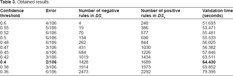
We executed the classification algorithm introduced in Section Methodology with minimum support threshold s _min = 0.9 and different values for the minimum confidence threshold cmin. For evaluating the performance of our approach, we have used the data set described in Subsection Data set and a cross-validation using a “leave-one-out” methodology was applied. Table 3 indicates the classification error obtained for different values for the minimum confidence threshold, the number of discovered rules in the training data as well as the validation time (the overall time in which PCRAR classifier performs the validation). We mention that our experiments were carried out on a PC at 3 GHz with 4 GB of RAM and that the validation time includes the computation time of the grid search procedure performed in order to find the optimal value for the correlation threshold ε. Because the number of negative and positive rules differs at each step in the cross-validation process (as a sequence is left out), we decided to indicate in Columns 3 and 4 in Table 3 the number of negative and positive rules generated in the entire training data sets DS_– and DS₊. The number of rules indicated in Columns 3 and 4 represents the maximum number of rules that are generated at a given step in cross-validation.

Table 3

Obtained results.

Confidence threshold	Error	Number of negative rules in DS–	Number of positive rules in DS +	Validation time (seconds)
0.6	4/106	4	240	51.693
0.55	5/106	19	386	53.471
0.52	6/106	70	577	55.481
0.5	6/106	134	690	55.533
0.48	6/106	262	844	56.025
0.47	3/106	431	1030	56.382
0.45	4/106	684	1226	57.846
0.42	3/106	1019	1434	63.511
0.4	2/106	1428	1689	64.430
0.38	3/106	1914	1973	69.852
0.36	6/106	2473	2292	79.395

The number of discovered binary relational association rules are indicated in Table 3. The rules discovered in the data set consisting of positive instances (belonging to the “+” class) will be referred to as positive rules and the rules discovered in the data set consisting of negative instances (belonging to the “-” class) will be referred to as negative rules.

As indicated in Table 3, the best result was obtained for a confidence threshold of 0.4, for which a classification error of 0.018867 (2/106) was reported after the validation was completed in 64.430 seconds. For the value 0.4 for confidence threshold the best value for the correlation threshold ε identified using the grid search procedure described above was ε = 10⁻² and this means that the attributes whose correlation with the target classification was below the threshold ε were eliminated during the pre-processing step.

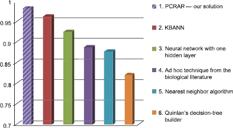
Compared to the classifiers already applied in the literature for promoter sequences recognition (see Table 2), the classifier introduced in this paper outperforms the best existing classifier for promoter sequences prediction: it is better than KB, ID3, O'Neill, NN and BP, considering the error of the classification. This comparison is illustrated in Figure 4. In this figure, the hatched bar indicates the performance of our PCRAR classifier.

Figure 4

Comparative results.

Another advantage of our approach compared to the existing approaches is that the training step of PCRAR is very fast, as it is enough to discover only binary relational association rules. It is very likely that the time needed to train our classifier (less than 2 minutes) is less than the training time of KB classifier.

The results described above bring us to the conclusion that applying relational association rule mining for promoter sequences prediction can lead to promising results and further improvements will, certainly, increase the accuracy of the obtained results.

Conclusions and Further Work

We have introduced in this paper a classification model based on relational association rules discovery for promoter sequences prediction. The experimental evaluation of the proposed model has shown that our classifier is better than the classifiers already applied for the considered problem, indicating the potential of our proposal.

The good performance of the classification model introduced in this paper leads us to the conclusion that machine learning models and data mining techniques are significant soft computing tools that are able to detect and recognize patterns in biological data, that are hard to be identified using other conventional computational techniques.

Further work will be made in order to identify and consider in the relational association rules discovery different types of relations between the nucleotides from a DNA sequence (from a biological or chemical point of view). ²⁷ We will also investigate how the confidence of the relational association rules discovered in the training data influences the accuracy of the classification task. Directions to hybridize our classification model, by combining it with other machine learning based predictive models ¹⁹ will be further considered.

Author Contributions

Conceived and designed the experiments: GC, MIB, IGC. Analysed the data: GC, MIB, IGC. Wrote the first draft of the manuscript: GC, MIB, IGC. Contributed to the writing of the manuscript: GC, MIB, IGC. Agree with manuscript results and conclusions: GC, MIB, IGC. Jointly developed the structure and arguments for the paper: GC, MIB, IGC. Made critical revisions and approved final version: GC, MIB, IGC. All authors reviewed and approved of the final manuscript.