CMCpy: Genetic Code-Message Coevolution Models in Python

Abstract

Code-message coevolution (CMC) models represent coevolution of a genetic code and a population of protein-coding genes (“messages”)- Formally, CMC models are sets of quasispecies coupled together for fitness through a shared genetic code. Although CMC models display plausible explanations for the origin of multiple genetic code traits by natural selection, useful modern implementations of CMC models are not currently available. To meet this need we present CMCpy, an object-oriented Python API and command-line executable front-end that can reproduce all published results of CMC models. CMCpy implements multiple solvers for leading eigenpairs of quasispecies models. We also present novel analytical results that extend and generalize applications of perturbation theory to quasispecies models and pioneer the application of a homotopy method for quasispecies with non-unique maximally fit genotypes. Our results therefore facilitate the computational and analytical study of a variety of evolutionary systems. CMCpy is free open-source software available from http://pypi.python.org/pypi/CMCpy/.

Introduction

Code-Message Coevolution (CMC) models were introduced to facilitate the study of co-evolutionary systems in which a large population of individuals share an evolvable genetic code coupled to many and/or long protein-coding genes (“messages”). Initial study of these models demonstrated that base mutations in protein-coding genes can significantly influence the fitness of genetic codes. ¹ More detailed study of CMC models has yielded formal demonstrations for how natural selection likely contributed to the origins of codon redundancy ² and non-random patterns of amino acid assignments^3,4 in genetic codes. CMC models have been extended to study the effects of population structure and gene sharing on coevolving systems of codes and messages. ⁵

In their original formulations, CMC models are deterministic evolutionary genetic models that couple together sets of large populations of asexually reproducing genotypes evolving under mutation and natural selection. One such population is called a “quasispecies”, ⁶ a concept reviewed recently both generally ⁷ and specifically in connection to population genetics theory.^8,9 In CMC models, each of multiple quasispecies represents a large population of codons evolving to meet the same physicochemical requirements of a “site-type” in proteins under translation by a given genetic code. The coupling of multiple quasispecies through a genetic code occurs through reuse of the same codon type (or allele) in different site-types. CMC models follow deterministic trajectories that alternate between equilibration of messages to an established genetic code by mutation and selection, and locally adaptive “gradient ascent” hill-climbing of the genetic code through single codon assignments and reassignments. This “quasistatic” dynamic continues until no single codon reassignment yields higher fitness with the current message population. Published CMC models always converge to a stable local fitness optimum–-a process called “code freezing.”

Because CMC models compound quasispecies models, analytical solutions to quasispecies models are relevant to their study. Previous applications of perturbation theory for approximate solutions to quasispecies models assume uniqueness of maximally fit genotypes and small perturbation parameters (small mutation rates).^10–12

In this work, we present two analytical methods that relax these assumptions. The first is a perturbative method that clarifies, extends and generalizes the perturbative approach to quasispecies models. Our presentation provides a derivation to arbitrary order, which relaxes any restriction on the magnitude of the perturbation parameter. The second method is the first published application of homotopy methods to quasispecies models, which handles cases with non-unique maximally fit genotypes. Numerical tests show that, for two example problems, both algorithms converge. Notably, the error of the perturbative method decreases exponentially in the number of iterations, suggesting its potential to outperform the power method. Both approaches are flexible and can be extended to a variety of quasispecies mutation models and fitness schemes. Also, both methods have been formulated so as to facilitate future connections between quasispecies models and established results in eigenvalue perturbation theory^13–15 and homotopy methods. ¹⁶

In addition to these analytical results, we present a new code-base implementing CMC models. The dissemination and further study of CMC models has been sorely hindered by the lack of a modern code-base implementing them. The original C/C++ CMC code-base has been rendered obsolete by evolution of compilers and language standards from the time of its writing in the late 1990s. This has created a need for reimplementation of the original models in an easy-to-use and program, powerful, and efficient, high-level scripting language like Python.

Here we present CMCpy, a free open-source code-base that implements CMC models in an easy to use object oriented Python API. The code-base comes with a front-end command-line executable called cmc that can drive the exploration of a variety of CMC models and reproduce published results.

Implementation

CMCpy was developed in Python 2.7. Figure 1 shows the organization of classes in CMCpy. A rich class hierarchy allows convenient specification of a wide-range of CMC models with very few lines of Python code.

Figure 1.

Overview of class hierarchy and containment relationships in CMCpy.

An element not shown in Figure 1 is that the ArdellSellaEvolver class is an abstract base class for a variety of subclasses implementing different strategies to solve dominant eigenpairs. The default solver relies on the Numpy eig() function for its speed and accuracy, but for reasons of flexibility, verification, and to experiment with different methods, we include a legacy central processing unit (CPU)-based power method, a multicore CPU-based power method implementation and an experimental graphics processing unit (GPU) implementation of the power method that relies on pyCUDA. ¹⁷

The pyCUDA solver is implemented in a CUDA C kernel with supportive Python code. The Python code uses NumPy for simple operations, to cast data to types acceptable by the CUDA platform, and to reshape matrices to one-dimensional data frames, for use by CUDA C. The CUDA C implementation of the power method approximately solves the eigenvector of each site-type, in parallel. Each site-type is assigned to one virtual “block” of the GPU, each of which corresponds to a physical processor when the number of blocks is below a hardware limit. This organization of the parallel workload was chosen to stay below CUDA specification limits, access GPU memory efficiently, and avoid excess complexity. Ultimately, the CUDA power method implementation is faster than the CPU power method implementation. Figure 2 shows system clock execution times of various methods on a 3.0 GHz Core 2 Duo with an Nvidia GeForce 460 GTX GPU running Ubuntu 12.04. The benchmark script in R that generated this figure is provided as supplementary data.

Figure 2.

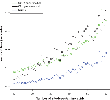
Comparison of wall-clock execution times of the cmc executable with three different eigensystem solvers using the double ring model ⁴ with eight codons, μ 0.1 and 0 = 0.25.

CMCpy comes with a front-end command-line executable in Python called cmc. This executable provides users, including non-programmers, the capability to reproduce (at least qualitatively) all of the published results on CMC models^1–4 as well as run individual and batch simulations of other models and parameter spaces. In Table 1 we list command-line options to the cmc executable and their corresponding model parameters.

Table 1.

Options to the cmc executable and corresponding model parameters.

Option	Long version	Description	Default
-a	—numaas	Number of amino-acids/site-types (AA/ST)	10
-d	—numdims	Dimensionality of AA/ST space	1
-s	— seed	Seed for random initialization of AA/ST coordinates	42
-t	—numtrials	Num. trials with reinitialized AA/ST spaces	1
-c	—numcodons	Num. codons in a “double ring” model	N/A
-b	—numbases	Alphabet size for word-based codon model	4
-P	—numpositions	Length of codons for word-based codon model	N/A
-m	—mu	Base (word models) or codon mutation rate	0.1
-k	—kappa	Transition/transversion mutation bias ratio	1
-f	—phi	Missense tolerance parameter	0.25
-r	—misreading	Misreading parameters	N/A

A variety of observables and statistics are implemented including the Normalized Encoded Range ² for one-dimensional amino acid/site-type spaces. Although CMC models are deterministic, exact quantitative differences may arise in results with CMCpy depending on floating point representation differences by platform and differences in convergence thresholds using power method-based eigensolvers.

It may be useful to restate the assumptions of the “Ardell-Sella” models currently implemented and available in CMCpy. These include the following:

1. 1.

The numbers and/or lengths of protein-coding genes, or “messages,” translated by a common genetic code, are large with respect to every possible site-type in proteins.

2.

For every possible site-type in proteins there corresponds a uniquely most fit amino acid.

3.

The machineries to decode codons, and to associate any codon to any amino acid, pre-exist the evolution of the genetic code.

4.

Fitness contributions of amino acids across sites are independent and multiplicative.

5.

Fitness contributions of different amino acids within the same site are independent and additive.

6.

Bases in messages mutate independently of one another.

7.

Messages are haploid and asexually reproducing.

8.

Genetic codes evolve much slower than messages, through discrete and independent assignments or reassignments of amino acids to codons.

Analytical Methods for Quasispecies Solutions

In this section we develop two different analytical methods to solve for the equilibrium growth rate and genotype distributions for a wide range of quasispecies models. The Matlab/Octave code used to implement these solutions are provided as supplementary data. A version of the homotopy method is also implemented in CMCpy for ring models. Full implementions of both methods will be incorporated into CMCpy at a later date.

Perturbative method: quasispecies with unique fittest genotype

We start with a ring mutation model discussed in prior work. ¹ Let μ denote the N x N mutation matrix

$$\mu =\left(\begin{array}{ccccc}1-2\mu & \mu & & & \mu \\ \mu & 1-2\mu & \mu & & \\ & \mu & \ddots & \ddots & \\ & & \ddots & 1-2\mu & \mu \\ \mu & & & \mu & 1-2\mu \end{array}\right),$$

(1)

where blank spaces should be interpreted as zeros. Throughout this derivation and the following one, we assume 0 ≤ μ < 1 and N > 1. Let w denote the N × N fitness matrix

$$w=\left(\begin{array}{ccc}{w}_1& & \\ & \ddots & \\ & & w_n\end{array}\right).$$

We assume that w₁ is the unique maximum of the finite set (w₁ …, w_N}. We also assume w > 0 for each i, consistent with prior work. ¹

Our goal in this derivation is to determine the leading eigenpair, consisting of the largest eigenvalue together with its corresponding eigenvector, of the matrix

$$\tilde{Q}\left(\mu \right)=\mu w.$$

(2)

We write $\tilde{Q}$ (μ) to emphasize the fact that since μ is a function of μ, so is Q. The diagonal matrix w is constant with respect to μ. Next we define

$$Q\left(\mu \right)=w^{1/2}\tilde{Q}\left(\mu \right)w^{-1/2}=w^{1/2}\mu w^{1/2}.$$

(3)

Since the matrices Q and Q are related by a similarity transformation, their eigenpairs are closely related. One can check that

$$Qv=\lambda v\hspace{1em}\text{if and only if}\hspace{1em}\tilde{Q}{w}^{-1/2}v=\lambda w^{-1/2}v$$

(4)

We focus our attention on Q because it is symmetric, i.e., Q(μ) ^T = Q(μ) for all μ.

For Q(μ), the leading eigenpair λ(μ), v(μ)) must satisfy

$$Q\left(\mu \right)v\left(\mu \right)=\lambda \left(\mu \right)v\left(\mu \right).$$

(5)

When μ = 0, the matrix μ reduces to the N x N identity matrix. Therefore, Q(0) = w, and the leading eigenpair of Q(0) is given by

$$\lambda \left(0\right)=w_1\hspace{1em}\text{and}\hspace{1em}v\left(0\right)=e_1.$$

(6)

Heree_j denotes the j-th basis vector in N-dimensional space, i.e., the vector with all zeros except for 1 in the j-th slot.

Guiding principle

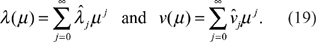
Since Q(μ) is symmetric for all real μ, standard theoretical results in eigenvalue perturbation theory ¹⁴ guarantee that both the eigenvalue λ(μ) and eigenvector v(μ) are analytic functions of μ. This means that there exists M > 0 such that for μ ∈ (-M, M), the following power series expansions converge:

$$\lambda \left(\mu \right)=\sum _{j=0}^{\infty }{\lambda }_j\frac{{\mu }^j}{j!}$$

(7a)

$$v\left(\mu \right)=\sum _{j=0}^{\infty }{v}_j\frac{{\mu }^j}{j!}$$

(7b)

In this notation, (6) can be written as λ₀ = w₁ and v₀ = e₁. Note also that we have arranged the coefficients so that

$${\frac{d^j}{d{\mu }^j}|}_{\mu =0}\lambda \left(\mu \right)={\lambda }_j$$

(8a)

$${\frac{d^j}{d{\mu }^j}|}_{\mu =0}v\left(\mu \right)=v_j$$

(8b)

Our strategy now will be to derive from (5) a recursive set of equations for the coefficients λ_j, μ_j. Once we have these coefficients for j = 0, 1, …, J, we have an approximation to the leading eigenpair.

Let I denote the n × n identity matrix. Then μ = 1 + μs, where

$$s=\left(\begin{array}{ccccc}-2& 1& & & 1\\ 1& -2& 1& & \\ & 1& \ddots & \ddots & \\ & & \ddots & -2& 1\\ 1& & & 1& -2\end{array}\right)\cdot$$

This implies that

$$\frac{d^j}{d{\mu }^j}\mu =\{\begin{array}{ll}s\hfill & j=1\hfill \\ 0\hfill & j\ge 2.\hfill \end{array}$$

By (3), we have

$$\frac{d^j}{d{\mu }^j}Q\left(\mu \right)=\{\begin{array}{ll}{w}^{1/2}s{w}^{1/2}\hfill & j=1\hfill \\ 0\hfill & j\ge 2.\hfill \end{array}$$

(9)

Perturbative solution: part I

Armed with the above facts, we differentiate (5) with respect to μ on both sides:

$$Q\text{'}\left(\mu \right)v\left(\mu \right)+Q\left(\mu \right)v\text{'}\left(\mu \right)=\lambda \text{'}\left(\mu \right)v\left(\mu \right)+\lambda \left(\mu \right)v\text{'}\left(\mu \right).$$

We then set μ = 0 and use (8), (3), (9), and (6) to obtain

$$w^{1/2}s{w}^{1/2}{e}_1+w{v}_1={\lambda }_1{e}_1+w_1{v}_1$$

(10)

Multiply this equation on the left by the row vector $e_1^T$ :

$$e_1^T{w}^{1/2}s{w}^{1/2}{e}_1+e_1^{T}w{v}_1={\lambda }_1+w_1{e}_1^T{v}_1.$$

(11)

Note that $e_1^T\text{W}=w_1{e}_1^T$ , which implies $e_1^T{\text{Wv}}_{\text{1}}=w_1{e}_1^T{v}_1$ . Using this equality in (11), we have

$$e_1^T{w}^{1/2}s{w}^{1/2}{e}_1={\lambda }_1.$$

This shows that if we already know (λ₀, v₀), we can determine λ₁. To determine v₁ we return to (10) except now we treat λ₁ as known. Rearranging the equation, we have

$$\left[w-w_{1}I\right]v_1=\left[{\lambda }_{1}I-w^{1/2}s{w}^{1/2}\right]e_1.$$

We substitute our definition of w on the left-hand side to obtain

$$\left(\begin{array}{ccccc}0& & & & \\ & w_2-w_1& & & \\ & & w_3-w_1& & \\ & & & \ddots & \\ & & & & w_N-w_1\end{array}\right)v_1=\left[{\lambda }_{1}I-w^{1/2}s{w}^{1/2}\right]e_1.$$

Suppose that v₁ = (v₁⁽¹⁾,v₁⁽²⁾,…, v₁^(N)). We set v₁⁽¹⁾=0. For the remaining components, we solve the above matrix-vector system to obtain

$$v_1^{\left(k\right)}=\frac{1}{w_k-w_1}{e}_k^T\left[{\lambda }_{1}I-w^{1/2}s{w}^{1/2}\right]e_1,\text{for }k=2,3,\dots ,N.$$

We have completed the loop, showing how to proceed from the zeroth-order eigenpair (λ₀, v₀) to the first-order eigenpair (λ₁,v₁).

In the next section, we show how to iterate this procedure to generate the j-th order eigenpair (λ_j, v_j) from the previously obtained eigenpairs.

Perturbative solution: part II

We return to (5) and take j derivatives with respect to μ on both sides. Using the general Leibniz rule, we have

$$\sum _{m=0}^j\left(\begin{array}{c}j\\ m\end{array}\right)\frac{d^m}{d{\mu }^m}Q\left(\mu \right)\frac{d^{j-m}}{d{\mu }^{j-m}}v\left(\mu \right)=\sum _{m=0}^j\left(\begin{array}{c}j\\ m\end{array}\right)\frac{d^m}{d{\mu }^m}\lambda \left(\mu \right)\frac{d^{j-m}}{d{\mu }^{j-m}}v\left(\mu \right)$$

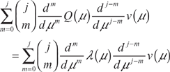
After differentiating, we set μ = 0 and use (8) to obtain

$$\sum _{m=0}^j\left(\begin{array}{c}j\\ m\end{array}\right)\frac{d^m}{d{\mu }^m}Q\left(\mu \right)v_{j-m}=\sum _{m=0}^j\left(\begin{array}{c}j\\ m\end{array}\right){\lambda }_m{v}_{j-m}$$

Applying (3) and (9) yields

$$w{v}_j+j{w}^{1/2}s{w}^{1/2}{v}_{j-1}=\sum _{m=0}^j\left(\begin{array}{c}j\\ m\end{array}\right){\lambda }_m{v}_{j-m}.$$

We peel off the m = 0 term from the right-hand side:

$$w{v}_j+j{w}^{1/2}s{w}^{1/2}{v}_{j-1}={\lambda }_0{v}_j+\sum _{m=1}^j\left(\begin{array}{c}j\\ m\end{array}\right){\lambda }_m{v}_{j-m}.$$

(12)

Multiplying on the left by $e_1^T$ and using $e_1^T\text{w}{v}_j=w_1{e}_1^T{v}_j={\lambda }_0{e}_1^T{v}_j$ , we see that the first term on the left-hand side cancels the first term on the right-hand side. We are left with

$$j{e}_1^T{\text{w}}^{1/2}{\text{sw}}^{1/2}{v}_{j-1}=\sum _{m=1}^{j-1}\left(\begin{array}{c}j\\ m\end{array}\right){\lambda }_m{e}_1^T{v}_{j-m}.$$

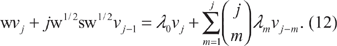
Now on the right-hand side, we peel off the m =j term—note that this the only term in which λ_j appears. Hence

$$j{e}_1^T{w}^{1/2}s{w}^{1/2}{v}_{j-1}=\sum _{m=1}^{j-1}\left(\begin{array}{c}j\\ m\end{array}\right){\lambda }_m{e}_1^T{v}_{j-m}+{\lambda }_j{e}_1^T{v}_0.$$

We use (6) and 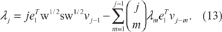$e_1^T{e}_1=1$ , and we solve for λ_j:

$${\lambda }_j=j{e}_1^T{w}^{1/2}s{w}^{1/2}{v}_{j-1}-\sum _{m=1}^{j-1}\left(\begin{array}{c}j\\ m\end{array}\right){\lambda }_m{e}_1^T{v}_{j-m}.$$

(13)

We have therefore shown that if we already know (λ_m, v_m) for m = 0, 1, …,j − 1, we can solve for λ_j. Now, using this λ_j, we can solve for v_j in the same way as before. We go back to (12), isolate all terms involving v_j, and apply (6) to derive

$$\left[w-w_{1}I\right]v_j=-j{w}^{1/2}s{w}^{1/2}{v}_{j-1}+\sum _{m=1}^j\left(\begin{array}{c}j\\ m\end{array}\right){\lambda }_m{v}_{j-m}$$

The right-hand side is clearly valid only for j ≥ 1. The matrix on the left-hand side is the same one that appeared earlier:

$$\left(\begin{array}{ccccc}0& & & & \\ & w_2-w_1& & & \\ & & w_3-w_1& & \\ & & & \ddots & \\ & & & & w_N-w_1\end{array}\right)v_j=-j{w}^{1/2}s{w}^{1/2}{v}_{j-1}+\sum _{m=1}^j\left(\begin{array}{c}j\\ m\end{array}\right){\lambda }_m{v}_{j-m}$$

We again set $v_j^{\left(1\right)}=0$ . For the remaining components, we have

$$v_j^{\left(k\right)}=\frac{1}{w_k-w_1}\left(-j{w}^{1/2}s{w}^{1/2}{v}_{j-1}+\sum _{m=1}^j\left(\begin{array}{c}j\\ m\end{array}\right){\lambda }_m{v}_{j-m}\right)$$

(14)

for k = 2, 3, …,N.

Algorithmic improvements

Equations (13) and (14) complete the step of deriving both (λ_j, v_j) using only the previously derived eigenpairs (λ_m, v_m for m = 0, 1, …j − 1, giving us a recursive solution procedure. Once we have determined (λ_j, v_j) for j = 0, 1, …, J, we can use these coefficients in (7) and thereby obtain approximations to the the leading eigenpair (λ(μ), v(μ)). Hence we view (13) and (14) as an algorithm for computing the leading eigenpair.

Turning to the numerical implementation, we now describe two improvements to the algorithm given by (13) and (14).

First, we note that in (14), we always set $v_j^{\left(1\right)}=0$ . This implies that $e_1^T{v}_j=0$ for all j ≥ 1. This means that all terms under the summation symbol in (13) vanish, yielding the simplified update formula:

$${\lambda }_j=j{e}_1^T{w}^{1/2}s{w}^{1/2}{v}_{j-1}.$$

(15)

Second, we note that (14) contains a binomial coefficient that becomes prohibitively large to compute for large j. A natural question is whether these large coefficients are compensated by the inverse factors of j! in (7). To quantify this, we define

$${\widehat{\lambda }}_j=\frac{{\lambda }_j}{j!}\hspace{1em}\text{and}\hspace{1em}{\widehat{v}}_j=\frac{v_j}{j!}.$$

(16)

We then substitute 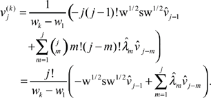${\lambda }_j=j!{\widehat{\lambda }}_j$ and $v_j=j!{\widehat{v}}_j$ in (14) and derive

$$\begin{array}{c}{v}_j^{\left(k\right)}=\frac{1}{w_k-w_1}\left(-j\left(j-1\right)!w^{1/2}s{w}^{1/2}{\widehat{v}}_{j-1}+\sum _{m=1}^j\left(\begin{array}{c}j\\ m\end{array}\right)m!\left(j-m\right)!{\widehat{\lambda }}_m{\widehat{v}}_{j-m}\right)\\ =\frac{j!}{w_k-w_1}\left(-w^{1/2}s{w}^{1/2}{\widehat{v}}_{j-1}+\sum _{m=1}^j{\widehat{\lambda }}_m{\widehat{v}}_{j-m}\right)\cdot \end{array}$$

Dividing through by j! and using (16), we derive, again for j ≥ 1,

$${\widehat{v}}_j^{\left(k\right)}=\frac{1}{w_k-w_1}\left(-w^{1/2}s{w}^{1/2}{\widehat{v}}_{j-1}+\sum _{m=1}^j{\widehat{\lambda }}_m{\widehat{v}}_{j-m}\right)\cdot$$

(17)

Applying the same substitutions in (15), we derive

$${\widehat{\lambda }}_j=e_1^T{w}^{1/2}s{w}^{1/2}{\widehat{v}}_{j-1}$$

(18)

Using (16) in (7), we obtain

$$\lambda \left(\mu \right)=\sum _{j=0}^{\infty }{\widehat{\lambda }}_j{\mu }^j\hspace{1em}\text{and}\hspace{1em}v\left(\mu \right)=\sum _{j=0}^{\infty }{\widehat{v}}_j{\mu }^j.$$

(19)

Examining the equations in the $\widehat{\lambda }$ and $\widehat{v}$ variables, we see that all large binomial coefficients and factorials have disappeared. For this reason, in our Octave implementation of the perturbative method, we use the recursive system given by (18) and (17), together with the summation formula (19). Finally, applying (4), our answer for the leading eigenpair of the matrix $\tilde{Q}$ (μ) defined by (2) is (λ(μ) w-^−1/2v(μ)).

Example

Let us give an example of the perturbative method in practice. We set N = 5, μ = 0.01, and w equal to a diagonal matrix whose entries along the diagonal are (φ, φ^d, φ^2d, φ^2d, φ^2d, φ^d) where d = 0.2 and φ = 0.32768.

Let J denote the total number of iterations we run the perturbative method. Starting from ${\widehat{\lambda }}_0=w_1$ and ${\widehat{v}}_0=e_1$ as in (6), we iterate using (18) and (17) from j = 1 up to j = J. We then evaluate the solution using (19) truncated at j = J, giving us an approximate solution that we denote (λ^J(μ), w^−1/2v^J(μ)).

For an N-dimensional vector x = (x₁, x₂, …, x_N), let ‖x‖_∞ = max_1≤i≤N, the infinity-norm of x, with respect to which the error of the approximate solution after J iterations is

$${\text{error}}^J={\Vert \mu w\left(w^{-1/2}{v}^J\left(\mu \right)\right)-{\lambda }^J\left(\mu \right)\left(w^{-1/2}{v}^J\left(\mu \right)\right)\Vert }_{\infty }.$$

In Figure 3, we plot (in circles) the log₁₀ of the error as a function of the number of iterations J, and (in solid black) the least-squares line of best fit to the data. From J = 1 to J = 14, the log₁₀ errors show a strongly linear trend, confirmed by the R ² = 0.9958 value for the regression line. The slope of the line is approximately −0.9944, implying

$${\text{error}}^J\propto {10}^{-0.9944J}.$$

Figure 3.

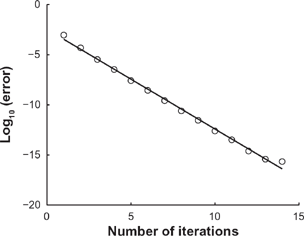
For a particular eigenvalue problem, we plot (in circles) the log₁₀ of the error committed by the the perturbative method after J iterations, where J goes from 1 to 14.

Machine epsilon in Octave is approximately 2.2204 × 10⁻¹⁶, and the error after J = 14 iterations is 2.2590 × 10⁻¹⁶. Therefore, for this particular example, Figure 3 shows that the perturbative method converges exponentially to a solution with error on the order of machine epsilon.

Extension to base/codon/word mutation models

Consider now a matrix μ_B defined as follows:

$${\mu }_B=\left(\begin{array}{cccc}1-\mu & \frac{k\mu }{k+2}& \frac{\mu }{k+2}& \frac{\mu }{k+2}\\ \frac{k\mu }{k+2}& 1-\mu & \frac{\mu }{k+2}& \frac{\mu }{k+2}\\ \frac{\mu }{k+2}& \frac{\mu }{k+2}& 1-\mu & \frac{k\mu }{k+2}\\ \frac{\mu }{k+2}& \frac{\mu }{k+2}& \frac{k\mu }{k+2}& 1-\mu \end{array}\right),$$

with constant parameters 0 < μ < 1 and k≥1, and the indexing of both rows and columns corresponding to bases in the ordered set B = (A, G, C, T). This matrix was employed in prior work ³ and corresponds to the Kimura two-parameter base mutation model. ¹⁸ When k = 1, μ_B represents the Jukes-Cantor mutation model. ¹⁹

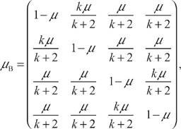
Matrix μ_B shares with matrix μ the properties of linearity in parameter μ, and reduction to the identity matrix when μ = 0. The methods of this section therefore apply to μ_B directly.

More biologically realistic CMC models^2–4 employ codon mutation models. Let C = B^p, the p-th Cartesian product of the set B. A codon c ∈ C is a string of bases b_lb₂…b_p of pre-specified length p with b_i ∈ B.

The codon mutation models studied by Ardell and Sella assume independence of mutation of bases within codons and that all bases mutate according to the same model of evolution μ_B. With these assumptions, mutation from any codon c₁, ∈ C to another codon c₂ ∈ C is represented by a matrix μ_c that is the p-th Kronecker power of a matrix μ_B as follows:

$${\mu }_C=\underset{i=1}{\overset{p}{\otimes }}{\mu }_B,$$

where (· ⊗ ·) is the Kronecker product, and codons are indexed in both rows and columns in lexicographic order.

If λ is the leading eigenvalue μ_B then λ_c = λ^p is the leading eigenvalue of μ_c. Similarly, if v is the eigenvector corresponding to the leading eigenvalue of μ_B, then $v_C={\otimes }_{i=1}^{p}v$ is the eigenvector corresponding to the leading eigenvalue of μ_c.

Therefore, the methods of this section allow calculation of the leading eigenpairs of matrices μ_c as Kronecker powers of leading eigenpairs of μ_B.

Homotopy method: quasispecies with multiple most fit genotypes

We now give a second method for finding the leading eigenpair of the matrix Q defined in (3). This method, which we call the homotopy method, is motivated by the desire to handle a fitness matrix w that does not have a unique maximal element along its diagonal. The homotopy method produces accurate approximations of the leading eigenpair for such problems.

Problem formulation

Our goal is still to find the leading eigenpair of $\tilde{Q}$ defined in (2). As before, we will instead focus our attention on the symmetric matrix Q defined by (3). We define the matrix-valued function

$$F(\in )=\mu +\in \left(w^{1/2}\mu w^{1/2}-\mu \right).$$

(20)

Note that F(0) = μ and F(1) = Q. The function F smoothly deforms μ into Q—such a function is often called a homotopy in the mathematical literature. ¹⁶ Note that for all ∈ ∈ [0,1], the leading eigenpair (λ(∈), v(e)) of F must satisfy

$$F(\in )v(\in )=\lambda (\in )v(\in ).$$

(21)

The basic idea behind the homotopy method is to use F to form a bridge between μ, a matrix whose leading eigenpair we already know, and Q, a matrix whose leading eigenpair we seek.

When ∈ = 0, (21) reduces to μv(0) = λ(0)v(0). By the results provided in supplementary materials, we know that the leading eigenvalue of F(0) = μ is 1 with corresponding eigenvector $\overrightarrow{1}={\left(1,1,\dots ,1\right)}^T$ , the column vector of N ones. This implies that

$$\lambda \left(0\right)=1\hspace{1em}\text{and}\hspace{1em}v\left(0\right)=\overrightarrow{1}.$$

(22)

When ∈ = 1, (21) reduces to Qv(1) = λ(1)v(1). Thus the question is how we can use our knowledge of (λ(0), v(0)) and the function F(∈) to derive (λ(1), v(1)), the leading eigenpair of Q.

Unlike the perturbative solution, at no point will we assume that the entries of w have a unique maximum. To make the derivation easier to read, we define

$$P=w^{1/2}\mu w^{1/2}-\mu ,$$

(23)

so that F(∈) = μ + ∈P and

$$F\text{'}(\in )=\frac{d}{d\in }F(\in )=P.$$

(24)

Homotopy solution

We differentiate both sides of (21) once with respect to ∈ and obtain

$$F\text{'}(\in )v(\in )+F(\in )v\text{'}(\in )=\lambda \text{'}(\in )v(\in )+\lambda (\in )v\text{'}(\in )$$

(25)

Since F(∈) is symmetric for all ∈, we see that the transposition of (21) can be written v(∈)^TF(∈) = λ(∈) v(∈) ^T . Thus, after multiplying (25) through on the left by v(∈)^T, the second term on the left-hand side cancels the second term on the right-hand side, leaving

$$\lambda \text{'}(\in )=\frac{v{(\in )}^{T}Pv(\in )}{v{(\in )}^{T}v(\in )}.$$

(26)

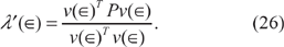
Now let us substitute (26) back into (25). Solving for v'(∈), we have

$$v\text{'}(\in )=-{\left[F(\in )-\lambda (\in )I\right]}^{-1}F\text{'}(\in )v(\in ).$$

(27)

We now recognize (26) and (27) as a system of ordinary differential equations (ODEs) with ∈ playing the role of a time-like independent variable:

$$\frac{d}{d\in }\left(\begin{array}{c}\lambda (\in )\\ v(\in )\end{array}\right)=\left(\begin{array}{c}\frac{v{(\in )}^{T}Pv(\in )}{v{(\in )}^{T}v(\in )}\\ -{\left[\mu +\in P-\lambda (\in )I\right]}^{-1}Pv(\in )\end{array}\right)$$

(28)

We also recognize (22) as the initial conditions for this system of ODEs. Let us now describe an elementary algorithm for solving this system:

1. 1.

Set λ = 1 and $v=\overrightarrow{1}$ . Fix an integer number of steps n_steps and then set Δ∈ = 1/n_steps. Also set ∈ = 0, initially.

2.

Whiles ∈ < 1:

• a.

  Compute λ′ using (26), i.e., λ′ = (v^TPv)/(v^Tv).

• b.

  Set λ ← λ + (Δ∈)λ.

• c.

  Using this updated λ, compute v' using (27), i.e., v' = -[μ+∈P-λI]⁻¹ Pv.

• d.

  Set v ← v+(Δ∈)v'.

• e.

  Set ∈ ← ∈ Δ∈.

The algorithm will terminate in n_steps steps, yielding an approximation to the leading eigenpair of Q that is stored in λ and v.

To obtain the leading eigenvector of $\tilde{Q}$ , we compute $\tilde{v}$ = w^−1/2v • The leading eigenpair of $\tilde{Q}$ is then (λ, $\tilde{v}$ ).

Example

We now give test results for the homotopy method applied to a particular problem. We set N = 8, μ = 0.1, and w equal to a diagonal matrix whose entries along the diagonal are (a, b, b, b, b, b, b, b) ^T with a = 0.63631836 and b = 0.73306514. We also set the parameter, φ = 1.

We repeatedly run the algorithm given above for different values of n_steps; specifically, we take n_steps = 10^j' j = 1, 2, 3, 4, 5, 6. For each value of n_steps, we compute an approximation to the leading eigenpair, which we denote by (λ ^j , v^j. We then evaluate the residual error of this approximation using

$${\text{error}}^j=\Vert \mu w\left(w^{-1/2}{v}^j\right)-{\lambda }^j\left(w^{-1/2}{v}^j\right)\Vert \infty .$$

In Figure 4, we plot (in circles) the log₁₀ of the error as a function of the log₁₀ of the number of steps. We also plot (in solid black) the least-squares line of best fit to the data; for this line, R ² = 0.9899 and the slope is approximately −1.0115, implying

$${\text{error}}^j\alpha n_{steps}^{-1.0115}\approx n_{steps}^{-1}=\Delta \in .$$

Figure 4.

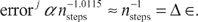
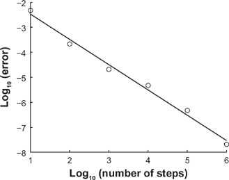
For a particular eigenvalue problem, we plot (in circles) the log₁₀ of the error committed by the the homotopy method using a number of steps given by n_steps = 10 ^j , where j goes from 1 to 6.

Note that with n_steps = 10 ³ , the error is approximately 2 × 10⁻⁵. This level of error is acceptable if we seek to use the homotopy method to reproduce, for example, Figure 4 in a previously published paper. ⁴ Hence we use this value of n _steps as the default value in the CMCpy implementation of the homotopy method.

Further note that when n_steps = 10 ⁶ , even the elementary algorithm described above to solve the system of nonlinear ODEs (28) is capable of producing a residual error of approximately 2 × 10⁻⁸.

For this example, the homotopy method displays convergence that is linear in Δ∈—-this relatively slow rate can be improved dramatically by using more sophisticated methods to solve the system of nonlinear ODEs (28), an issue we leave for future work.

Extension to base/codon/word mutation models

In order to apply the homotopy method to models where the mutation matrix is given by μ_B as defined earlier, there is one requirement: we must be sure that μ_B has a unique maximal eigenvalue of 1. For the μ_B matrix, it turns out that we can explicitly derive all eigenvectors and eigenvalues, for general values of both μ and k. With the constraints 0 < μ < 1 and k ≥ 1, the derivation that we give in supplementary materials below proves that the μ_B matrices have a unique largest eigenvalue of 1. Matrices μ_B therefore fulfill the minimum requirements for applicability of the methods of this section, after which the leading eigenpair for corresponding matrices μ_C may be calculated using Kronecker powers as before.

Future outlook

We succeeded in programming a GPU-based power method implementation that is faster than its CPU analogue; however, the performance gain that we obtained with it was not as great as we had hoped. Furthermore, even though our implementation is correct, we could not completely eliminate divergence in evolutionary trajectories in power method implementations arising from differences in machine number representations and precision across platforms. We believe that this arises from deviations in the way double precision floating point numbers are represented, computed on, and rounded in CUDA compute capability 1.3. Perhaps utilization of the cuBLAS library in the future would make performance closer to Numpy and better conform to IEEE standards.

Furthermore, while the power method converges linearly, our new perturbation method provides exponential convergence with the same accuracy. However, this method cannot handle the case of non-unique most fit genotypes that occurs in CMC models at their initialized state. On the other hand, our new homotopy method does handle this case, yet as currently implemented it also converges linearly, rather slower than the power method (results not shown). Incorporation of more sophisticated methods to solve systems of nonlinear ordinary differential equations should dramatically improve performance of our new homotopy method application. We leave further development of both methods and their implementation in CMCpy for future work; perhaps other CPU or GPU implementations of them will compete with Numpy. More generally, our analytical results greatly expand the domain of quasispecies models that can be accurately solved using analytical approaches, particularly multi-site models with biologically realistic mutation parameters.

A variety of open problems remain concerning CMC models and in the field of the evolution of the genetic code.^20–24 CMCpy can easily be extended to implement the model studied by Vetsigian et al. (2006) ⁵ with variations, or alternative observables, such as the “evenness” of amino acids. ²³ Current models of the genetic code have not yet integrated a theory for the origin of translation per se.^5,21 We believe that extensions to CMC models will better address such fundamental questions and hope that CMCpy and our analytical solutions to quasispecies models will play a role in that work.

Funding

DHA acknowledges the UC Merced division Graduate Research Council for a UC Faculty Research and Chancellor's awards that supported undergraduate BPS, as well as the NSF-funded program in Undergraduate Research in Computational Biology at UC Merced (DBI-1040962), which supported and trained PJB and paid publication costs.

Competing Interests

Author(s) disclose no potential conflicts of interest.

Author Contributions

Conceived CMCpy project: DHA. Wrote software: DHA, PJB, BPS. Analyzed data: DHA, HSB, PJB, BPS. Analytical results: HSB, with minor contributions from DHA. Wrote first draft of the manuscript: DHA, HSB. Contributed to the writing of the manuscript: DHA, HSB. Agree with manuscript results and conclusions: DHA, HSB, PJB, BPS. Developed the structure and arguments for the paper: DHA, HSB. Made critical revisions and approved final version: DHA, HSB, PJB. All authors reviewed and approved of the final manuscript.

Disclosures and Ethics

As a requirement of publication author(s) have provided to the publisher signed confirmation of compliance with legal and ethical obligations including but not limited to the following: authorship and contributorship, conflicts of interest, privacy and confidentiality and (where applicable) protection of human and animal research subjects. The authors have read and confirmed their agreement with the ICMJE authorship and conflict of interest criteria. The authors have also confirmed that this article is unique and not under consideration or published in any other publication, and that they have permission from rights holders to reproduce any copyrighted material. Any disclosures are made in this section. The external blind peer reviewers report no conflicts of interest.