Sage Journals: Discover world-class research

Abstract

A mathematical formalism describing the nonlinear end-systolic pressure–volume relation (ESPVR) is used to derive new indexes that can be used to assess the performance of the heart left ventricle by using the areas under the ESPVR (units of energy), the ordinates of the ESPVR (units of pressure), or from slopes of the curvilinear ESPVR. New relations between the ejection fraction (EF) and the parameters describing the ESPVR give some insight into the problem of heart failure (HF) with normal or preserved ejection fraction. Relations between percentage occurrence of HF and indexes derived from the ESPVR are also discussed. When ratios of pressures are used, calculation can be done in a noninvasive way with the possibility of interesting applications in routine clinical work. Applications to five groups of clinical data are given and discussed (normal group, aortic stenosis, aortic valvular regurgitation, mitral valvular regurgitation, miscellaneous cardiomyopathies). No one index allows a perfect segregation between all clinical groups, it is shown that appropriate use of two indexes (bivariate analysis) can lead to better separation of different clinical groups.

Keywords

pressure–volume relation PVR ventricular mechanics heart failure ESPVR mathematical physiology segregation and classification of clinical data

Introduction

There have been extensive studies published in the literature on the problem of heart failure with normal or preserved ejection fraction (HFpEF) defined as ejection fraction (EF) >50%, and about half the patients with symptoms of heart failure (HF) have normal or near-normal EF.^1–6 It was first reported by Dumesnil et al.^7–9 that patients with aortic stenosis can have decrease in longitudinal shortening and wall thickening of the left ventricle, while the EF remains within normal limits because of intrinsic factors and/or left ventricular geometry.^10,11 One should not lose sight of the fact that HF is complex process that involves interacting factors like the intrinsic state and metabolism of the myocardium, relaxation mechanism, ventricular filling and ejection, preload, and afterload. In this study we look at HFpEF from one angle, it is the relation between EF and indexes derived from the end-systolic pressure–volume relation (ESPVR) that in some way reflects the state of the myocardium.

When the myocardium reaches its maximum state of activation during the contraction phase, the relation between pressure and volume is known as the ESPVR as explained in more detail in the next section. The application of the ESPVR to clinical problems is not new.^12–18 In the case of a linear approximation of the ESPVR, studies have focused usually on the use of the maximum slope E_max and the volume axis intercept V_om for assessing the performance of the left ventricle, for a review see^13,19 and a tutorial introduction can be found in.²⁰ The interesting observation that the curvilinearity of the ESPVR contains information that reflects in some way the contractility of the myocardium has been reported,^21–25 a point that will be given some attention in this study. Mathematical relations between EF and the parameters describing the ESPVR have been discussed in previous studies by the author both in case of linear ESPVR^26,27 and in case of nonlinear ESPVR.²⁸ It was shown that the EF is just one of several indexes that can be derived from the ESPVR for assessing the state of the myocardium. In this study, some of these indexes are reviewed and new applications to clinical data published in the study by Dumesnil et al.^7–9 are presented that show the consistency of the mathematical formalism used. Moreover, it is shown that when ratios of parameters involving pressures or areas are used, the indexes derived from the ESPVR can be calculated in a noninvasive way from volume measurements only, for instance, by using echocardiography or magnetic resonance imaging. The mathematical formalism developed applies also to the right ventricle^29–31 and possibly to the four chambers of the heart, and the discussion in this study is confined to the left ventricle. A minimal number of equations are used in the main text to describe the properties of the ESPVR, and more complex mathematical formalism is confined to Supplementary Material.

Mathematical Model

Unlike most studies on the topic, our approach to the problem was mainly theoretical.^{25–28,31–39} As shown in Figure 1, the left ventricle is represented as a thick-walled cylinder contracting symmetrically, a helical muscular fiber in the myocardium is projected as a dotted circle on the cross-section. Because of the symmetry assumption, a radial active force/unit volume of the myocardium D(r) is generated, and it will develop an active pressure on the inner surface of the myocardium (endocardium), expressed as follows

\int_{a}^{b} D (r) d r = \bar{D} h

(1)

Figure 1.

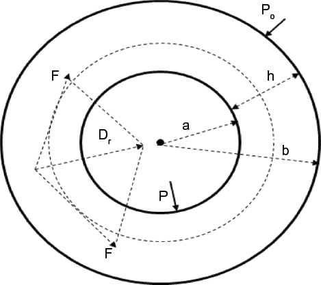
Cross-section of a thick-walled cylinder representing the myocardium. The dotted circle represents the projection of a helical muscular fiber on the cross-section of the myocardium. D_r is the radial active force/unit volume of the myocardium. P is the ventricular pressure, P_o is the external pressure on the epicardium (assumed zero), a = inner radius, b = outer radius, h = b - a = thickness of the myocardium.

The thickness of the myocardium is given by h = b - a, where a = inner radius of the myocardium, b = outer radius, and $\bar{D}$ is an average radial active force/unit volume of the myocardium calculated by applying the mean value theorem. In a quasi-static approximation of the contraction (inertia and viscous forces neglected), we can write $\bar{D} h \approx P_{i s o}$ , where P_iso is the notation used by physiologists to indicate the isovolumic pressure developed by the myocardium in a nonejecting contraction. Near end-systole when the myocardium reaches its maximum state of activation with maximum isovolumic pressure P_isom and left ventricular pressure P_m, the equilibrium of forces on the inner surface of the myocardium can be expressed as follows

P_{i s o m} - P_{m} = E_{2 m} (V_{e d} - V_{m})

(2)

P_m is assumed constant during the ejection phase for simplicity as shown in Figure 2, the corresponding left ventricular volume is V_m ≈ V_es (end-systolic volume when Vd/dt = 0), V_ed, is the end-diastolic volume (when dV/dt = 0), and SV ≈ V_ed - V_m is the stroke volume. The elastance coefficient E_2m = tanβ₂ is the slope of the line CD shown in Figure 2. If P_isom is kept constant in Equation (2) and the point D with coordinates (P_m, V_m) is varied from (0, V_om) to (P_isom, V_ed) in Figure 2 (as if a balloon was inflated against a constant P_isom), we get the ESPVR represented by the curve BDC. The ESPVR curve is tangent to the P-V loop at the point (P_m, V_m), and the P-V loop of a normal ejecting contraction is represented in a simplified way in Figure 2 by the rectangle V_edD₁DV_m. Two other relations can be obtained by splitting Equation (2) as follows

P_{m} = E_{1 m} (V_{m} - V_{o m}) = E_{2 m} (V_{m} - V_{o 2})

(3)

P_{i s o m} = E_{m} (V_{e d} - V_{o m}) = E_{2 m} (V_{e d} - V_{o 2})

(4)

Figure 2.

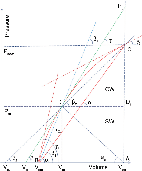
Curvilinear ESPVR represented by the curve BDC, B is the intercept with the volume axis (corresponding to V_om). For simplicity, the ventricular pressure P_m is assumed constant during the ejection phase, P_isom is the peak isovolumic pressure, P_t corresponds to the ordinate of the intercept of the tangent with the vertical line AC. Stroke work SW ≈ P_m (V_ed - V_m), area PE = arc(BD)V_mB. Total area TW = arc(BDC)AB, area CW = TW - PE - SW. The tangent (with slope tanγ) to the curve BDC at point (P_m, V_m) intersects the horizontal volume axis at V_ot, the line DC (with slope tanβ₂) intersects the horizontal volume axis at V_o2, and the line BD (with slope tanβ₁) intersects the horizontal volume axis at V_om. Units of volume are ml and units of pressure are mmHg

The elastance coefficients E_1m = tanβ₁ (slope of the line BD) and E_m = tanα (slope of the line BC) are shown in Figure 2 as well as the intercept V_om of the curvilinear ESPVR with the volume axis; V_o2 corresponds to the intercept of the line CD with the volume axis. Unlike the linear ESPVR that is described by one slope E_max,^33–35 the nonlinear ESPVR (curve BDC in Fig. 2) can be described by several slopes that are summarized as follows:

\tan α = \frac{P_{i s o m}}{V_{e d} - V_{o m}} = slope of the line CB

(5a)

e_{a m} = \frac{p_{m}}{S V} = arterial elastance near end-systole

(5b)

\tan β_{1} = \frac{P_{s} - P_{m}}{S V} = \frac{P_{s}}{V_{e d} - V_{o m}} = \frac{P_{m}}{V_{m} - V_{o m}}

(5c)

where P_s corresponds to the ordinate of the intercept of the line BD with the vertical line AC (not shown in Fig. 2). We also have

\tan β_{2} = \frac{P_{i s o m} - P_{m}}{S V} = \frac{P_{i s o m}}{V_{e d} - V_{o 2}} = \frac{P_{m}}{V_{m} - V_{o 2}}

(5d)

where V_o2 corresponds to the intercept of the line CD with the volume axis. Finally,

\tan γ = \frac{d P_{m}}{d V_{m}} = \frac{P_{t} - P_{m}}{S V} = \frac{P_{t}}{V_{e d} - V_{o t}} = \frac{P_{m}}{V_{m} - V_{o t}}

(5e)

is the slope of the tangent to the ESPVR at point D with coordinates (P_m, V_m), P_t corresponds to the ordinate of the intercept of the tangent with the vertical line AC, and V_ot corresponds to the intercept of the tangent with the volume axis.

\tan γ_{1} = \tan gent to the ESPVR at po int B

(5f)

\tan γ_{3} = \tan gent to the ESPVR at po int C

(5g)

Expressions for tanγ, tanγ₁, and tanγ₃ are given in the Supplementary Material and in Shoucri.²⁸

Stroke Volume

The following relations can be easily derived from the preceding equations:

\frac{\tan β_{2}}{e_{a m} + \tan β_{2}} = \frac{S V}{V_{e d} - V_{o 2}} \frac{P_{i s o m} - P_{m}}{P_{i s o m}}

(6a)

\frac{\tan γ}{e_{a m} + \tan γ} = \frac{S V}{V_{e d} - V_{o t}} \frac{P_{t} - P_{m}}{P_{t}}

(6b)

\frac{\tan β_{1}}{e_{a m} + \tan β_{1}} = \frac{S V}{V_{e d} - V_{o m}} \frac{P_{s} - P_{m}}{P_{s}}

(6c)

Equation (6) show how the ratios of the afterload measured by the stroke volume SV to the preload measured by V_ed - V_o2, V_ed - V_ot, or V_ed - V_om are determined by the ratios of the slopes describing the ESPVR and how the inotropic state of the myocardium as expressed by the peak isovolumic pressure P_isom is related to the parameters describing the ESPVR (Equation (6a)). These complex relations are similar to the relation derived in the case of a linear ESPVR: SV = (V_ed -V_o) E_max/(e_am + E_max) (see Sunagawa et al.¹⁸). For the sake of completeness, we give also the following relation that can be derived for a cylindrical model and that shows the influence of the geometry on the calculation of SV:

S V = S V R + \frac{1}{8} V_{ω} Δ (\frac{h}{R})

(7)

SVR is the stroke volume of the mid-wall cylinder with radius R = (a + b)/2, V_ω is the volume of the myocardium assumed constant and δ(h/R) is the variation of the ratio h/R between end-diastole and end-systole. Equations (6) and (7) reflect the complex interrelation between several factors affecting the SV, and consequently, the EF = SV/V_ed. Equation (7) shows that ratios of volumes like SV/V_ω or SVR/V_ω can be calculated from transversal M-mode echocardiographic measurement of h/R as explained in Dumesnil et al.^7–9

Stroke Work

The stroke work SW ≈ P_m (V_ed - V_m) is a measure of the energy delivered to the systemic circulation during the contraction phase. In Figure 2, when the point D with coordinates (P_m, V_m) moves along the ESPVR (curve BDC), the stroke work SW reaches its maximum value SW_x, with corresponding values P_m = P_mx, V_m = V_mx, when the following condition is satisfied:

\frac{d (S W)}{d V_{m}} \approx \frac{d}{d V_{m}} [P_{m} (V_{e d} - V_{m})] = (V_{e d} - V_{m}) \frac{d p_{m}}{d V_{m}} - P_{m} = 0

(8)

By using Equations (5b) and (5e), we get when SW = SW_x

\tan γ_{x} = e_{a m x}

(9)

A similar relation has been obtained in the case of a linear ESPVR.^26,27,34,35 The stroke work reserve SWR is defined as in the case of linear ESPVR as follows:

S W R = S W_{x} - S W \approx P_{m x} (V_{e d} - V_{m x}) - P_{m} (V_{e d} - V_{m})

(10)

SWR is an important index to assess the ventricular function. It measures the ability of the ventricle to increase its output as a result of an increase in load demand measured by an increase in P_m. Similar to the linear model of ESPVR,^26,27,34,35 one can distinguish the following cases in studying the performance of the ventricle: a.

tanγ > e_am, which corresponds to P_m < P_mx, V_m < V_mx, and SW < SW_x. It corresponds to a normal state of the ventricular function. An increase in P_m due to an increase in load demand results in a corresponding increase in the stroke work SW.

tanγ_x ≈ e_amx, which corresponds to P_m ≈ P_mx, V_m ≈ V_mx, and SW ≈ SW_x. It corresponds to a mildly depressed state of the heart. An increase in P_m due to an increase in load demand results in a decrease in SW, resulting in cardiac insufficiency.

tanγ < e_am, which corresponds to P_m > P_mx, V_m > V_mx, and SW < SW_x. It corresponds to a severely depressed state of the heart. An increase in P_m due to an increase in load demand results in a severe decrease in SW causing severe cardiac insufficiency.

Experimental verification of these results for the left ventricle can be found in Asanoi et al.¹² and Burkhoff and Sagawa⁴⁰ and for the right ventricle in Brimioulle et al.²⁹

Applications to Clinical Data

Clinical data measured by M-mode echocardiography on patients corresponding to five clinical groups are taken from results published in Dumesnil et al.^7–9 They have been used to calculate the results shown in Table 1 and in the figures. The echocardiographic measurements consisted in the transversal dimensions of the myocardium (inner and outer radii, thickness). The longitudinal axis was calculated in Dumesnil et al.^7–9 by angiography for the purpose of validating the equations used. A cylindrical model was used to calculate the volume of the myocardium V_ω as reproduced in the second column of Table 1. A cylindrical model was also used to calculate V_ed, and V_m in Table 1. However, it should be clear that calculating ratios of volumes, ratios of slopes, ratios of areas under the ESPVR, or ratios of pressures can be done in a noninvasive way as is evidenced from Equation (6), the equations given in the Supplementary Material based on a cylindrical model, and as explained in Dumesnil et al.^7–9 Moreover, one can find several studies about the estimation of the ventricular volume or the length of the longitudinal axis from measurement of the transversal dimensions of the myocardium.

Table 1.

Results of calculation of different variables used in the study of various clinical groups.

	LVID MM	V_{ω ML}	V_edML	V_mML	V_omML	V_otML	tanα/e_am	P_isom/P_m	P_T/P_M
Normal subjects
1	47	136.5	181.7	56.2	37.8	28.7	2.04	2.33	5.57
2	52	203.8	247.8	76.6	51.5	39.1	2.05	2.35	5.57
3	42	130.8	134.4	55	37.2	28.6	1.79	2.19	4.01
4	46	135.5	170.9	51.5	34.6	26.3	2.07	2.36	5.74
5	48	181	198.2	57	38.2	29	2.12	2.41	6.04
6	51	154.5	229	94.2	64.1	49.1	1.75	2.14	3.99
7	52	181	244.5	84	56.7	43.2	1.94	2.27	4.94
8	45	177.3	167.1	50.5	33.8	25.7	2.1	2.4	5.71
9	52	178.2	244	86.3	58.3	44.5	1.91	2.25	4.76
Aortic stenosis
1	38	211.4	112.9	17.6	11.6	8.7	2.61	2.78	11.7
2	43	222.8	154.4	56.1	37.6	28.9	1.96	2.33	4.61
3	38	166.8	108.1	26.9	17.9	13.6	2.31	2.56	7.06
4	41	165.9	130.4	43.7	29.3	22.4	2.02	2.36	5.06
5	41	194.3	133.8	42	28	21.4	2.11	2.43	5.46
6	39	194.3	118.3	38	25.3	19.4	2.1	2.43	5.32
7	42	326.1	156.2	50.1	33.3	25.5	2.12	2.46	5.32
8	49	285.3	222.8	44	29.1	21.9	2.44	2.64	9.12
9	58	358.3	355.2	121.5	81.6	62.4	1.98	2.32	4.96
10	43	177.3	149.2	30.9	20.5	15.4	2.4	2.61	8.67
11	49	306.2	225.9	103.9	70.3	54.5	1.67	2.13	3.47
12	48	610.4	244.2	120	80.7	63.4	1.61	2.12	3.19
Aortic valvular regurgitation
1	71	354.5	605.5	238.1	162.5	124.1	1.78	2.15	4.22
2	59	305.2	364	90.97	60.8	45.94	2.22	2.46	7.06
3	78	464.5	802.8	195	131	98.73	2.18	2.41	7.32
4	57	317.5	334.2	112.3	75.53	57.65	1.99	2.32	5.06
5	53	196.2	260.1	83.24	56.1	42.67	2.01	2.31	5.36
6	60	413.3	395.5	116.5	77.94	59.26	2.12	2.41	5.87
Mitral valvular regurgitation
1	76	488.2	751.9	284.6	193.4	147.5	1.83	2.19	4.41
2	54	250.2	281.8	75.43	50.46	38.23	2.18	2.44	6.55
3	58	193.4	331	142.7	97.62	74.66	1.68	2.09	3.77
4	59	239.8	354.3	107.7	72.61	55.07	2.04	2.33	5.69
Miscellaneous cardiomyopathies
1 (MVP)	43	99.53	138.2	60.87	41.52	31.89	1.68	2.1	3.67
2 (MVP)	48	202.8	201.4	77.1	51.98	39.87	1.87	2.24	4.34
3 (CM)	68	264.5	524.5	322.1	224.9	174.4	1.2	1.77	2.37
4 (IHSS)	38	189.6	110.6	21.13	13.97	10.51	2.5	2.7	9.43
5 (IHSS)	28	53.1	41.75	4.823	3.182	2.368	2.69	2.81	16.04
6 (IHSS)	38	139.3	104.8	9.497	6.258	4.638	2.77	2.86	20.61
7 (IHSS)	38	263.5	117.6	41.45	27.62	21.256	2.03	2.4	4.77
8 (IHSS)	44	256.9	167.8	66.17	44.41	34.257	1.87	2.27	4.18
9 (DSAS)	42	165.9	139	31.87	21.18	16	2.33	2.57	7.75

Abbreviations: LVID, left ventricular internal diameter in diastole; V_ω, volume of the myocardium; V_ed, end-diastolic volume; V_m ≈ V_es, end-systolic volume; V_om abscissa of the intercept of ESPVR with the volume axis; V_ot, abscissa of the intercept of the tangent at point (P_m, V_m) to the ESPVR with the volume axis; P_t ordinate of the intercept of the tangent at point (P_m, V_m) to the ESPVR with the vertical axis through V_ed (Fig. 2); P_isom, peak isovolumic pressure; P_m, left ventricular pressure corresponding to the ESPVR. Units of volume are ml, and units of pressure are mmHg. Calculation is based on data taken from Dumesnil et al.^7–9 MVP, mitral valve prolapsed; CM, cardiomyopathy; IHSS, idiopathic hypertrophic subaortic stenosis; DSAS, discrete subaortic stenosis.

The left ventricular pressure P_m has not been measured with the data given in Dumesnil et al.^7–9 Results of calculation for P_isom/P_m and P_t/P_m given in Table 1 were obtained by using Equation (6).

Calculation of V_om, V_o2, V_ot: The calculation of the intercept V_om of the ESPVR with the volume axis is carried out by using the Newton–Raphson method to calculate the root of a nonlinear equation as explained in Shoucri.^28,36–39 The algorithm also calculates V_o2 and V_ot by using, for instance, Equations (4), (5d), and (5e), and the results are shown in Table 1. Figure 3 shows the relation between y = (P_isom - P_m)/P_m against x = SV/(V_m - V_o2) derived from Equation (6a). It was found that transforming an index x into the form x1 = x/std(x) (std = standard deviation, in this case std(x1) = 1 and mean(x1) = mean(x)/std(x)) or into the form x1 = (x + mean(x))/std(x) (in this case std(x1) = 1and mean(x1) = 2 mean(x)/std(x)), can give better separate display of clinical groups as shown in Figure 3.

Two-dimensional display of data allows better segregation between clinical groups. This property is further illustrated in Figure 4, where the plotting of EF versus EF/std(EF), and (V_m - V_o2)/V_o2, versus [(V_m - V_o2)/V_o2]/std[(V_m - V_o2)/V_o2] is shown. Notice for instance in Figure 4 (left) that the projection of the data along the horizontal axis (EF) or vertical axis (EF/std(EF)) introduces overlap between the different clinical groups, but the two-dimensional display shows a clear segregation between the five clinical groups. However, we introduce in this way a problem of classification, given a new piece of data how to choose the standard deviation to place it in one of the groups displayed. But there are other statistical methods that can be used for classification, like cross-validation, bootstrap analysis, and areas under ROC curves.

Bivariate analysis of data: In Figure 5 the same parameters are used in the left side and right side; however, the grouping of data is different on the left side and the right side depending on the clinical groups considered. Notice in Figure 5 (left) that values of (P_isom - P_m)/TW (resultant pressure on the endocardium/total area under the ESPVR) appear enhanced for some cases of aortic stenosis with respect to the normal group and that smaller values of (P_isom - P_m)/TW correspond to larger values of SV indicating a possible increase in time in order to achieve ejection.

Stroke work reserve, SWR: Figure 6 (left) shows a relation between SWR/SW and EF = SV/V_ed. Figure 6 (right) shows a relation between SWR/SW and tanγ/e_am. Notice from Figure 6 (left) that SWR/SW → 0 for EF ≈ 0.33 ≈ 1/3, and from Figure 6 (right) that SWR/SW →; 0 when tanγ/e_am →;1 in agreement with Equations (8) and (9).

Occurrences of HF: Figure 7 (left) shows the percentage of occurrences of HF plotted against LVEF (left ventricular ejection fraction [%], data taken from Figure 1.1 of Da Mota³) (see also a similar graph in Curtis et al.²). We have then calculated a least square fit of the data that is shown by the solid curve in Figure 7 (left). This least square fit was then used to calculate the percentage of occurrences of HF for the EFs of the five clinical groups considered in this study. The results are shown in Figure 7 (right). The results on both sides of Figure 7 indicate a minimum of occurrences of HF around EF ≈ 0.66 ≈ 2/3. Figure 8 (left) shows the calculated percentage of occurrences of HF plotted versus 100*SWR/SW for the five clinical cases considered in this study. A minimum of the curve is observed around SWR/SW ≈ 0.3. Figure 8 (right) shows the calculated percentage of occurrences of HF plotted versus 100*(V_ed - V_mx)/SV, a minimum of the curve is observed around (V_ed - V_mx)/SV ≈ 0.79 (or SV/(V_ed - V_mx) ≈ 1.25). In Figure 9 (left), the percentage of occurrences of HF/respective standard deviation of each group is plotted versus 100*EF for the five clinical groups considered in this study, and in Figure 9 (right) a similar plot versus 100*SWR/SW is shown. The highest curve in the graphics (normal case) results from the fact that this clinical group has the smallest standard deviation. Notice that in the five clinical cases shown in Figure 9, the minima of the curves occur around EF ≈ 0.67 and around SWR/SW ≈ 0.3. Figure 10 (left) shows the calculated percentage of occurrences of HF plotted versus 100*SV/(V_ed - V_om) for the five clinical cases considered in this study, a minimum of the curve is observed around SV/(V_ed - V_om) ≈ 0.85. Figure 10 (right) shows the calculated percentage of occurrences of HF plotted versus 100*SV/(V_ed - V_o2), a minimum of the curve is observed around SV/(V_ed - V_o2) ≈ 0.57.

Figure 3.

(Left) Variation of y = (P_som - P_m)/P_m against x = SV/(V_m - V_o2); better segregation between clinical groups can be obtained by plotting y/std(y) against x (center) and (y + mean(y))/std(y) against (x + mean(x))/std(x) (right) for each clinical group; normal case *, aortic stenosis o, aortic valvular regurgitation +, mitral valvular regurgitation ^, miscellaneous cardiomyopathies x.

Figure 4.

(Left) Relation between EF and EF/std(EF). (Right) Relation between (V_m - V_o2/V_ed and [(V_m - V_o2)/V_ed]/std([(V_m - V_o2)/V_ed]); normal case *, aortic stenosis o, aortic valvular regurgitation +, mitral valvular regurgitation ^, miscellaneous cardiomyopathies x.

Figure 5.

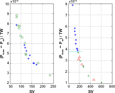
(Left) Plot of (P_isom - P_m)/TW versus stroke volume SV, no segregation of data between normal group (*) and aortic stenosis (o) is observed. (Right) Segregation of data indicated by the horizontal line between normal group (*) and aortic valvular regurgitation (+), and mitral valvular regurgitation (^). Notice that by using the same coordinates, one can get different segregation of clinical data depending on the clinical groups considered; some indexes appear to be more appropriate to separate between some clinical groups than others.

Figure 6.

(Left) Relation between SWR/SW and EF, notice that SWR/SW → 0 around EF → 0.33 ≈ 1/3. (Right) Relation between SWR/SW and tanγ/e_am, notice that SWR/SW → 0 around tanγ/e_am → 1; normal case *, aortic stenosis o, aortic valvular regurgitation +, mitral valvular regurgitation ^, miscellaneous cardiomyopathies x.

Figure 7.

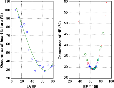
(Left) Percentage of occurrences of HF versus left ventricular ejection fraction LVEF (%) as calculated from Da Morta³, solid line corresponds to least square fit of data. (Right) Percentage of occurrences of HF versus percentage of ejection fraction 100*EF for five clinical groups, calculated with the least square fit shown by the solid curve on the left side, based on data taken from Dumesnil et al^7–9; normal case *, aortic stenosis o, aortic valvular regurgitation +, mitral valvular regurgitation ^, miscellaneous cardiomyopathies x.

Figure 8.

(Left) Percentage of occurrences of HF versus 100*SWR/SW. (Right) Percentage of occurrences of HF versus 100*(V_ed – V_mx)/SV. Notice the minimum of the curve in each case around the normal group; normal group *, aortic stenosis o, aortic valvular regurgitation +, mitral valvular regurgitation ^, miscellaneous cardiomyopathies x.

Figure 9.

Percentage of occurrences of HF / respective standard deviation of each group, for the five clinical groups considered in this study, versus left ventricular ejection fraction EF (%) (left), and SWR/SW (%) (right); normal case *, aortic stenosis o, aortic valvular regurgitation +, mitral valvular regurgitation ^, miscellaneous cardiomyopathies x.

Figure 10.

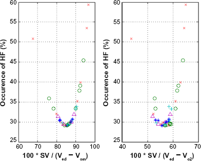
(Left) Percentage of occurrences of HF versus 100*SV/(V_ed – V_om). (Right) Percentage of occurrences of HF versus 100*SV/(V_ed - V_o2). Notice the minimum of the curve in each case around the normal group; normal group *, aortic stenosis o, aortic valvular regurgitation +, mitral valvular regurgitation ^, miscellaneous cardiomyopathies x.

Discussion

This study has shown that the EF is just one of a rich collection of indexes that can be derived from the parameters describing the nonlinear ESPVR as shown in Figure 2. These parameters in some way reflect the state of the myocardium. The results of this study indicate that there is not a single index that can give a full discriminate separation between all clinical groups. Good segregation from the normal group depends on the clinical group and the index used. Some interesting results have been obtained: a.

Two-dimensional graphic representations of data by using two indexes can give better segregation between clinical groups (instead of using just one index like EF), which suggests the idea that bivariate (or multivariate) analysis may be a better approach to study the classification of clinical data than univariate analysis. In particular instead of using an index x, the use of x/std(x) or (x + mean(x))/std(x) can give better segregation between clinical groups (see Figs.).

When the left ventricular pressure P_m is not measured, the factor k_w cannot be calculated in Equations (A1)-(A7) in the Supplementary Material and only ratios of quantities involving pressures or areas can be calculated. This is also evident from Equation (6). These ratios may have a reduced sensitivity to reflect the intrinsic state of the myocardium by eliminating k_w. But this drawback can be compensated by the fact that the obtained indexes can be calculated in a noninvasive way. Notice that P_m can be approximated, for instance, by using the peak blood pressure.

Numerical values of some indexes given at the end of the previous section should be considered as preliminary results that need further experimental confirmation. However, there is a consistency in the results obtained, for instance, the stroke work reserve SWR = SW_x - SW → 0 for tanγ/e_am → 1 (see Fig. 6 [right]) has been verified in a previous study on other clinical data.²⁸ Also from the study of linear ESPVR^26,27,34,35 and experimental results,^12,29,40 we know that the ratio E_max/e_am (maximum elastance/arterial elastance) for the normal state of the heart is of order of ≈ 2, which corresponds to the results of this study that show that tanα/e_am is varying between 1.75 and 2.1 (see Table 1).

The variation of percentage of occurrences of HF with various indexes presented in Figures 7–10 shows consistency. Notice that the normal group (*) appears around the minimum of all the curves shown in the Figures 7 (right) to 10, which is an indication of the consistency of the calculations. The HF patients contain cases with HFpEF (also referred to as diastolic HF), as is evidenced from the overlap around EF ≈ 0.67 between normal group and cases of cardiomyopathies shown in Figures 7–10.

Notice that the formalism used in this study has allowed the classification of the performance of the ventricle in normal, mildly depressed, and severely depressed state as discussed at the end of Mathematical Model section, and the introduction of the concept of stroke work reserve (SWR) that can help in assessing the ventricular function. The introduction of the isovolumic pressure P_isom in the formalism describing the PVR as in Equation (2) is an important feature of the mathematical formalism used. Discussion of these results can be found in previous publications.^{26–28,34,35}

This study has shown relations between stroke volume SV (and EF = SV/V_ed) and parameters describing the ESPVR, which opens a new and interesting direction of research in the study of the problem of HFpEF. Both the diastolic and systolic state of the myocardium will influence the shape of the ESPVR. More experimental and clinical observations are needed to understand the complex interrelation between the indexes presented in this study and how they can be used to predict HFpEF.

Conclusion

An important feature of the mathematical formalism presented in this study is that it gives a new insight in the mechanics of ventricular contraction. The study of the ESPVR offers a rich collection of parameters that can be exploited in a noninvasive way in order to assess the state of the myocardium and the pump function of the heart. Not one of the indexes introduced in this study can allow full separation between all clinical groups, but some indexes appear to be more appropriate for some clinical groups than others. It turns out that bivariate (or multivariate) analysis of data is superior to univariate analysis (like using only EF) for the purpose of segregation between different clinical groups. The implication of these results for the study of the problem of HFpEF has been indicated and need further research for full assessment.

Supplementary Material

The slope of the line CD is E_2m = tanβ₂ (see Equation (2) and Fig. 2) and it is given by Equation (25) of Shoucri.³²

\tan β_{2} = k_{w} (\frac{1}{V_{m}} - \frac{1}{V_{m} + V ω} + \frac{1 n (\frac{V_{e d}}{V_{m}}) - 1 n (\frac{V_{e d} + V_{ω}}{V_{m} + V_{ω}})}{V_{e d} - V_{m}})

(A1)

V_w is the volume of the myocardium assumed constant, the coefficient k_w = (∂W/∂I)_av is an average value calculated by applying the mean value theorem, W is the pseudo-strain energy function of the passive medium of the myocardium, and I is the first strain invariant and appearing as a multiplicative geometrical factor. When we let V_m → V_om in Equation (A1), we get the expression of the slope E_m = tanα of the line BC (see Equation (4) and Fig. 2)

\tan α = k_{w} (\frac{1}{V_{o m}} - \frac{1}{V_{o m} + V_{ω}} + \frac{h (\frac{V_{e d}}{V_{o m}}) - h (\frac{V_{e d} + V_{ω}}{V_{o m} + V_{ω}})}{V_{e d} - V_{o m}})

(A2)

Notice that along the line BC, the slope tanα is constant, and consequently, k_w is constant. We have assumed that along the ESPVR represented by the curve BDC in Figure 2, we can take k_w as nearly constant. By writing P_m = P_isom - (P_isom - P_m) and by using Equations (2), (4), (A1), and (A2), we get for the expression of left ventricular pressure P_m along the curve BDC

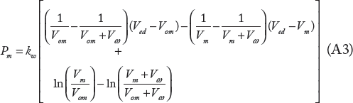
P_{m} = k_{w} [\begin{array}{l} (\frac{1}{V_{om}} - \frac{1}{V_{om} + V_{ω}}) (V_{e d} - V_{o m}) - (\frac{1}{V_{m}} - \frac{1}{V_{m} + V_{ω}}) (V_{e d} - V_{m}) \\ 1 n (\frac{V_{m}}{V_{o m}}) - 1 n (\frac{V_{m} + V_{ω}}{V_{o m} + V_{ω}}) \end{array}]

(A3)

When V_m → V_ed, we get the expression for the peak volumic pressure

P_{i s o m} = k_{w} [(\frac{1}{V_{o m}} - \frac{1}{V_{o m} + V_{ω}}) (V_{e d} - V_{o m}) + 1 n (\frac{V_{e d}}{V_{o m}}) - 1 n (\frac{V_{e d} + V_{ω}}{V_{o m} + V_{ω}})]

(A4)

By calculating ratios P_isom/P_m or tanα/tanβ, the factor k_w is eliminated. These ratios and similar ratios can be calculated in a noninvasive way by measuring the dimensions of the left ventricle. Equations (A3) and (A4) are used to calculate V_om by using an iterative process as in Shoucri.^28,38,39 For the slope tanγ = dP_m/dV_m of the tangent to the ESPVR, we get

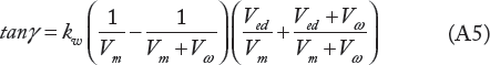
\tan γ = k_{w} (\frac{1}{V_{m}} - \frac{1}{V_{m} + V_{ω}}) (\frac{V_{e d}}{V_{m}} + \frac{V_{e d} + V_{ω}}{V_{m} + V_{ω}})

(A5)

When V_m →; V_om in Equation (A5), we get the slope tanγ₁ of the tangent to the ESPVR at point B (see Fig. 2)

\tan γ_{1} = k_{w} (\frac{1}{V_{o m}} - \frac{1}{V_{o m} + V_{ω}}) (\frac{V_{e d}}{V_{o m}} + \frac{V_{e d} + V_{ω}}{V_{o m} + V_{ω}})

(A6)

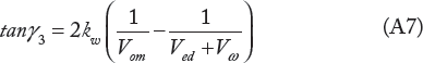
When V_m → V_ed in Equation (A5), we get the slope tanγ₃ of the tangent to the ESPVR at point C (see Fig. 2)

\begin{matrix} \tan γ_{3} = 2 k_{w} (\frac{1}{V_{o m}} - \frac{1}{V_{e d} + V_{ω}}) \end{matrix}

(A7)

Author Contributions

Conceived and designed the experiments, data taken from Dumesnil et al.^7–9 Analyzed the data: RMS. Wrote the first draft of the manuscript: RMS. Contributed to the writing of the manuscript: RMS. Agree with manuscript results and conclusions: RMS. Jointly developed the structure and arguments for the paper: RMS. Made critical revisions and approved final version: RMS. The author reviewed and approved of the final manuscript.

References

Bhatia

R.S.

, Tu

J.V.

, Lee

D.S.

Outcome of heart failure with preserved ejection fraction in a population-based study. N Engl J Med. 2006; 355(3): 260–9.

Curtis

J.P.

, Sokol

S.I.

, Wang

The association of left ventricular ejection fraction, mortality, and cause of death in stable outpatients with heart failure. J Am Coll Cardiol. 2003; 42(3): 736–42.

Da Mota

JPGF

Intelligent Modeling to Predict Ejection Fraction from Echocardiographic Reports [MSc thesis]. Portugal: Mechanical Engineering, IST Técnico Lisboa; 2013.

Manisty

C.H.

, Francis

D.P.

Ejection fraction: a measure of desperation. Heart. 2008; 94: 400–1.

Najjar

Heart failure with preserved ejection fraction. J Am Coll Cardiol. 2009; 54: 412–9.

Sanderson

J.E.

Heart failure with normal ejection fraction. Heart. 2007; 93: 155–8.

Dumesnil

J.G.

, Shoucri

R.M.

, Laurenceau

J.L.

, Turcot

A mathematical model of the dynamic geometry of the intact left ventricle and its application to clinical data. Circulation. 1979; 59: 1024–34.

Dumesnil

J.G.

, Shoucri

R.M.

Effect of the geometry of the left ventricle on the calculation of the ejection fraction. Circulation. 1982; 65: 91–8.

Dumesnil

J.G.

, Shoucri

R.M.

Quantitative relationship between left ventricular and wall thickening and geometry. J Appl Physiol. 1991; 70: 48–54.

10.

Coppola

B.A.

, Omens

J.H.

Role of tissue structure on ventricular wall mechanics. Mol Cell Biomech. 2008; 5: 183–96.

11.

Jones

C.J.H.

, Raposo

, Gibson

D.G.

Functional importance of the long axis dynamics of the human left ventricle. Br Heart J. 1991; 63: 215–20.

12.

Asanoi

, Sasayama

, Kamegama

Ventriculo-arterial coupling in normal and failing heart. Circ Res. 1989; 65: 91–8.

13.

Burkhoff

, Mirsky

, Suga

Assessment of systolic and diastolic ventricular properties via pressure-volume analysis: a guide for clinical, translational, and basic researchers. Am J Physiol Heart Circ Physiol. 2005; 289: H501–12.

14.

De Tombe

P.P.

, Jones

, Burkhoff

, Hunter

W.C.

, Kass

D.A.

Ventricular stroke work and efficiency both remain nearly optimal despite altered vascular loading. Am J Physiol. 1993; 264: H1817–24.

15.

Klautz

R.J.

, Verwey

H.F.

, van der Wall

E.E.

, Dion

R.A.

, Steendijk

Single-beat estimation of the left ventricular end-systolic pressure-volume relationship in patients with heart failure. Acta Physiol. 2010; 198: 37–46.

16.

Suga

Cardiac energetic: from Emax to pressure-volume area. Clin Exp Pharmacol Physiol. 2003; 30: 580–5.

17.

Suga

Global cardiac function: mechano-energetics-informatics. J Biomech. 2003; 36: 713–20.

18.

Sunagawa

, Maughan

W.L.

, Sagawa

Optimal arterial resistance for the maximal stroke work studied in isolated canine left ventricle. Circ Res. 1985; 56: 586–95.

19.

Kjorstad

K.E.

, Korvald

, Myrmel

Pressure-volume-based single-beat estimation cannot predict left ventricular contractility in vivo. Am J Physiol Heart Circ Physiol. 2002; 282: H1739–50.

20.

Sagawa

The end-systolic pressure-volume relation of the ventricle: definition, modifications and clinical use. Circulation. 1981; 63: 1223–7.

21.

Burkhoff

, Sugiura

, Yue

D.T.

, Sagawa

Contractility-dependent curvilinearity of end-systolic pressure-volume relations. Am J Physiol Heart Circ Physiol. 1987; 252: H1218–27.

22.

Kass

D.A.

, Beyar

, Lankford

, Heard

, Maughan

W.L.

, Sagawa

Influence of contractile state on curvilinearity of in situ end-systolic pressure-volume relations. Circulation. 1989; 79: 167–78.

23.

Noda

, Cheng

, De Tombe

P.P.

, Little

W.C.

Curvilinearity of LV end-systolic pressure-volume and dP/dtmax-end-diastolic volume relations. Am J Physiol Heart Circ Physiol. 1993; 265: H910–7.

24.

Sato

, Shishido

, Kawada

ESPVR of the in situ rat left ventricle shows contractility-dependent curvilinearity. Am J Physiol Heart Circ Physiol. 1998; 274: 1429–34.

25.

Shoucri

R.M.

Non-linear pressure-volume relation in left ventricle. Jpn Heart J. 1991; 32: 337–46.

26.

Shoucri

R.M.

ESPVR, ejection fraction and heart failure. Cardiovasc Eng. 2010; 10: 207–12.

27.

Shoucri

R.M.

Basic relations between ejection fraction and ESPVR. Austin J Clin Cardiol. 2014; 1(5): 1–6.

28.

Shoucri

R.M.

Ejection fraction and ESPVR: a study from a theoretical perspective. Int Heart J. 2013; 54(5): 318–27.

29.

Brimioulle

, Waulthy

, Ewalenko

Single-beat estimation of right ventricular end-systolic pressure-volume relationship. Am J Physiol Heart Circ Physiol. 2003; 284: H1625–30.

30.

Maughan

W.L.

, Shoukas

A.A.

, Sagawa

, Weisfeldt

Instantaneous pressure-volume relationship of the canine right ventricle. Circ Res. 1979; 44: 309–15.

31.

Shoucri

R.M.

Pressure-volume relation in the right ventricle. J Biomed Eng. 1993; 15: 167–9.

32.

Shoucri

R.M.

Theoretical study of the pressure-volume relation in left ventricle. Am J Physiol Heart Circ Physiol. 1991; 260: H282–91.

33.

Shoucri

R.M.

Clinical application of end-systolic pressure-volume relation. Ann Biomed Eng. 1994; 22: 212–7.

34.

Shoucri

R.M.

Possible clinical applications of the external work reserve. Jpn Heart J. 1994; 35: 771–7.

35.

Shoucri

R.M.

Studying the mechanics of left ventricular contraction. IEEE Eng Med Biol Mag. 1998; 17: 95–101.

36.

Shoucri

R.M.

Numerical evaluation of the slope and intercept of end-systolic pressure-volume relation. In: Brebbia

C.A.

, ed. Environmental Health & Biomedicine (Biomed 2011, 26-28 July, Riga, Latvia). Southampton, Boston: WIT Press; 2011: 333–45.

37.

Shoucri

R.M.

A non-invasive method to calculate parameters of non-linear end-systolic pressure-volume relation. Int J Cardiol. 2011; 151: 389–91.

38.

Shoucri

R.M.

A method to calculate the parameters of non-linear ESPVR in the ventricles I. In: Rivas-Echeverria

, Allegaert

, Wainstein

D.E.

, eds. Proceedings of the World Medical Conference, September 26–28. Prague, Czech Republic; 2011: 142–9.

39.

Shoucri

R.M.

A method to calculate the parameters of the isovolumic curves in the ventricles II. In: Rivas-Echeverria

, Allegaert

, Wainstein

D.E.

, eds. Proceedings of the World Medical Conference, September 26–28. Prague, Czech Republic; 2011: 150–5.

40.

Burkhoff

, Sagawa

Ventricular efficiency predicted by an analytical model. Am J Physiol. 1986; 250: R1021–7.

End-systolic Pressure–Volume Relation,Ejection Fraction,and Heart Failure: Theoretical Aspect and Clinical Applications

Abstract

Keywords

Introduction

Mathematical Model

Stroke Volume

Stroke Work

Applications to Clinical Data

Discussion

Conclusion

Supplementary Material

Author Contributions

References