Sage Journals: Discover world-class research

Abstract

Reverse phase protein arrays (RPPA) measure the relative expression levels of a protein in many samples simultaneously. Observed signal from these arrays is a combination of true signal, additive background, and multiplicative spatial effects. Background subtraction alone is not sufficient to remove all nonbiological trends from the data. We developed a surface adjustment that uses information from positive control spots to correct for spatial trends on the array beyond additive background. This method uses a generalized additive model to estimate a smoothed surface from positive controls. When positive controls are printed in a dilution series, a nested surface adjustment performs an intensity-based correction. When applicable, surface adjustment is able to remove spatial trends and increase within slide replicate agreement better than background subtraction alone as demonstrated on two sets of arrays. This work demonstrates the importance of including positive control spots on the array.

Keywords

protein array normalization control spots generalized additive models

Introduction

Protein arrays are assays that measure protein expression in a high-throughput format. These are able to address questions about postranslational modifications and protein pathway relationships that genomic studies alone cannot answer.¹ Several different protein array formats have been developed, but they can be generally dichotomized into forward phase or reverse phase assays. Forward phase assays simultaneously measure the levels of many proteins or antibodies within a single sample, where as reverse phase assays simultaneously measure the level of a single protein for many samples. One reverse phase approach that uses lysed homogenized samples is the protein lysate or reverse phase protein array (RPPA) first described by Paweletz et al.²

RPPAs have been used to research a number of biological issues. For example, RPPAs were used to study proteomic signatures of signaling pathways in prostate cancer.^2,3 Nishizuka et al⁴ used RPPAs to find molecular markers that can distinguish colon from ovarian cancer, two types of cancer that at onset are difficult to separate. Gulman et al⁵ found unique proteomic signatures that were able to distinguish fast progressing follicular lymphoma from slow progressing disease. Other studies found proteins that play key roles in the regulation of pathways in different types of cancer including breast cancer,⁶ glioma,⁷ and leukemia.⁸ More studies using RPPAs include.^9–15

The RPPA assay is described in detail by Paweletz et al,² Tibes et al,¹⁶ and in several review articles.^17–19 For the specific methods we use, see Tibes et al.¹⁶ Briefly, sample lysates are spotted onto a nitrocellulose backed array in a dilution series. The array is then hybridized with a specific rigorously validated antibody manufactured to recognize the protein of interest. Protein signal is amplified starting with a biotinylated secondary antibody that binds to the primary antibody. Next, a streptavidin-biotin complex binds to the secondary antibody and produces a visible precipitate after chemical processing. The processed array is scanned on an ordinary flatbed scanner and the resulting image is quantified with MicroVigene (VigeneTech, Inc., North Billerica, MA), an array software that measures the intensity of the label at each spot on the array. The array software provides measurements of both foreground and background intensities at each spot, where the local background at a spot is the intensity measured just outside a printed spot.

In the RPPA setting, a false positive signal can occur for one of two reasons. First, either the primary antibody binds to an incorrect target and the secondary antibody and biotin complex react appropriately to this misbound antibody or, second, the secondary antibody and biotin complex, alone or in combination, bind promiscuously and deposit signal in a process that is independent of the primary antibody. The first cause, incorrect binding of the primary antibody, has been addressed by using only antibodies that have been strictly validated using a Western blot. The vigorous validation scheme used to screen antibodies is described in detail by Tibes et al.¹⁶ The binding of the primary antibody to an incorrect target is not generally a concern in the RPPA setting. It is the second cause, the undiscriminate binding of secondary antibody or biotin complex, that is of major concern in this paper. When these substances react with the nitrocellulose membrane or with contaminants in the non-print areas of the array, regional non- specific signal will be detected that could make the data unuseable. Figure 1 shows an RPPA that exhibits this global patchy signal across the slide that must be dealt with. In general, the data from “dirty” slides, such as the one in Figure 1, will be usable once the regional non-specific non-print area staining is appropriately accounted for.

Figure 1.

An example RPPA slide that shows visible regional non-print area staining.

The usual approach for adjusting for these spatial artifacts is through background correction, which is accomplished by subtracting the local background intensity at a spot from the foreground intensity of that spot. Figure 2 illustrates the importance of background correction for RPPAs. The figure shows Bland-Altman plots²⁰ of biological replicates that were printed on different parts of the array for four example RPPAs both before and after subtracting local background signal from the foreground signal. Each of these slides were printed with protein from the same samples, but different antibodies were used to measure different proteins on each slide. Clearly, inter-slide reproducibility is vastly improved after background correction, especially for Array C. However, some slides (for example, Array A and Array B) suggest background subtraction alone is not sufficient.

Figure 2.

Bland-Altman plots of replicates on four arrays. Each row represents a separate array. The first column shows replicate agreement before any correction, the center column shows replicate agreement after background subtraction, and the third column shows replicate agreement after surface adjustment. While background subtraction improves agreement, the off-center B-A plots of the center column indicate remaining spatial artifacts that are removed with surface correction.

In the presence of regional non-print area staining, low expressions will not be detected because they are dominated by the spatial background, although the strongest signals will still be discernible. Figure 3 illustrates this concept using three ficticious samples with high, moderate and low levels of protein, each in 5-spot dilutions. The right column of Figure 3 shows the cumulative effect of protein expression dependent on differing degrees of non-specific background staining representing 0%, 25%, 50% and 75% of maximum signal strength. Even at the highest level of background, the strongest signals are still discernible, but the signal from the higher dilutions or from samples with lower abundance become disproportionately overwhelmed by the levels of background. In this paper, we propose a method to correct the regional spatial effects with a multiplicative model using high expression control spots (positive controls) on the array. The proposed method is able to appropriately account for the spatial non-print area staining effects that would otherwise prevent use of the data.

Figure 3.

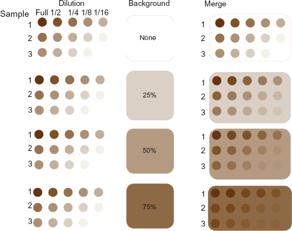
Effect of different background levels on overall signal. In this schematic, three samples with high, moderate and low levels of protein are shown as they would appear on the array with the 5 dilutions. Differing degrees of non-specific background staining representing 0%, 25%, 50% and 75% of maximum signal strength are shown in the center. On the right side, the cumulative effect of the actual protein dependent staining and the non-specific background are shown merged. Even at the highest level of background, the strongest signals are still discernible, but the signal from the higher dilutions or from samples with lower abundance become disproportionately overwhelmed by the levels of background.

Methods

Data

This study uses data from two separate RPPA experiments. The first dataset is a collection of 52 arrays described by Kornblau et al⁸ and Kornblau and Coombes.²¹ Each array contains 550 patient samples printed in duplicate on separate sections of the array. The 52 slides represent the different antibodies with which the arrays were probed. The second dataset is also described by Kornblau and Coombes.²¹ The number of samples included in this dataset necessitated printing on two slides, so for the 138 antibodies used, a total of 276 slides were stained. There were 1152 samples printed on the two slides (576 samples per slide) in replicate.

Both sets of arrays were printed, processed, and analyzed using methods previously described in Tibes et al,¹⁶ Kornblau et al,⁸ and Kornblau and Coombes.²¹

Positive Controls

The positive control spots on the arrays from this study were made from a mixture of cell lines designed to have levels of all proteins of interest. As a result, the PC spots printed on the arrays will always be expressed. Furthermore, when there is more than one PC spot on an array, they should all be expressed at the same level.

Negative control (NC) spots are spots on the array that are printed with buffer. NC spots, therefore, should not bind to antibodies and can also be another estimate of background signal. Buffer is used as the NC to aid in determining where the non-print signal is coming from.

This paper examines the spatial effects of two RPPA datasets. The first is a set of 52 arrays, each printed in the format of Design I. Design I has 8064 spots in a 56 × 144 grid. Each 14 × 12 subgrid (shown in Figure 4, left) contains 28 samples printed in a 5-spot dilution series. Each dilution series is followed alternatively by a PC or a NC spot. There are 48 subgrids on the array, each with 14 PC and 14 NC spots for a total of 672 PC and 672 NC on the array.

Figure 4.

Subgrid layout of two array designs. The left layout (Design I) prints a full strength positive control (red) or negative control (white) at the end of each dilution series (gray). The right layout (Design II) prints the positive control spots in a 5-spot dilution series (red and pink).

The second dataset is a collection of 276 arrays, each printed in the format of Design II. Design II has 6912 spots in a 48 × 144 grid. Each of the 48 subgrids on the array (see Figure 4, right) has 24 samples printed in a 5-spot dilution series. Each dilution series is followed by either a NC, a PC, or a diluted PC spot. The PC spots are printed at full, 1/2, 1/4, 1/8, and 1/16 strength dilutions (see Figure 5). There are 4 NC spots and 4 PC spots at each of the 5 dilution strengths on the subgrid for a total of 192 NC spots and 192 PC spots at each dilution strength.

Figure 5.

Positive control (PC) expression for a slide with low regional variation. The PC dilution is fairly linear on average. The 1/2 strength dilution is expressed at the same level as the full strength because both are protein saturated.

With RPPA data, a simple additive correction for background is sometimes not sufficient to remove all spatial trends from the signal. Figure 2 shows that there are remaining artifacts that background subtraction does not fully correct. These effects are generally from non-print area staining, although other factors such as uneven hybridization will occasionally contribute. Empirical evidence suggests that spots with more protein are more affected by non-print area spatial staining than low expression spots.

We use the following equation to model the relationship between observed signal intensity, background, spatial effects, and true signal intensity:

Y_{i j}^{r c} = Y_{i j} * P^{r c} + B G^{r c}

(1)

where $Y_{i j}^{r c}$ is the observed intensity of sample j at dilution step i, also dependent on the physical row r and column c of the spot on the array; Y_ij is the desired spatially independent signal; P^rc is the effect of non-print area staining; and BG^rc is background signal. From this point on, it is assumed that the observed $Y_{i j}^{r c}$ has had the background subtracted, so the relationship simplifies to $Y_{i j}^{r c} = Y_{i j *} P^{r c}$ . The goal is to recover Y_ij, so that analysis can be done on spatially independent observations.

Surface Adjustment

The assumption for recovery of Y_ij is that the PC spots (of the same dilution strength) are expressed at the same intensity. Prior data suggests that PC expression has a CV of less than 6%–15% and dot size variation is very low. Therefore, we use the PC spots to estimate the spatial surface needed to adjust the observed intensities in order to return spatially independent values. We will first discuss an adjustment method for Design I arrays, in which PCs are only printed at full strength. Next, we will discuss a method for Design II arrays, in which PCs are spotted at different dilution strengths. In both cases, PC spots expressed below the 75 percentile of the negative control expression were not used.

Design I methods

The Design I array has 14 full strength PC spots and 140 spots with biological samples, both in full and diluted strengths in each subgrid (see Figure 4). To do the spatial adjustment, we need a PC estimate, ${\hat{P}}^{r c}$ , for each spot on the array. That is, we need to estimate the intensity that would have been expressed had the spot in row r and column c been printed as a PC. One way to do this is to assign ${\hat{P}}^{r c}$ at each spot the value of the PC closest in distance. This approach, however, can be improved with smoothing techniques.

We used a generalized additive model (GAM) to build a smooth surface from which to estimate PC values at each spot on the array. For the GAM, $Y_{i j}^{r c}$ was modelled as a smooth function of the row and column coordinates of the positive controls. We used the R package mgcv²² to obtain model estimates. With the estimated model, we obtain predicted PC values at each spot on the array. Let ${\hat{P}}^{r c}$ be the predicted PC value obtained from the surface. The spatial effects were removed by scaling each $Y_{i j}^{r c}$ by the amount needed to atten the estimated PC surfaces, or rather to set each ${\hat{P}}^{r c}$ to the same value, here arbitrarily chosen to be the median value of the surface. The spatially independent intensities are obtained by dividing observed values by the estimated PC and multiplying by the median PC value: $Y_{i j} = Y_{i j}^{r c} / {\hat{P}}^{r c}$ median $(\hat{P})$ .

Design II methods

When the PC spots are printed in a dilution series, the levels of positive controls are exploited to perform an intensity-based adjustment. We first build PC surfaces at each dilution level using the predicted values from a GAM as explained previously. Let ${\hat{P}}_{[1]}$ be the surface built from the undiluted spots, ${\hat{P}}_{[2]}$ be the surface built from the 1/2 strength spots, and so on to ${\hat{P}}_{[5]}$ , the surface built with the 1/16 strength spots. The surfaces are constrained to not cross, so that

{\hat{P}}_{[1]}^{r c} > {\hat{P}}_{[2]}^{r c} > {\hat{P}}_{[3]}^{r c} > {\hat{P}}_{[4]}^{r c} > {\hat{P}}_{[5]}^{r c} .

In practice, if ${\hat{P}}_{[k]}^{r c} < {\hat{P}}_{[k + 1]}^{r c}$ we set ${\hat{P}}_{[k + 1]}^{r c} = {\hat{P}}_{[k]}^{r c} - \in$ with some small ∈.

Next, each spot is scaled to the surface it is closest to in intensity. When the observed intensity falls between two surfaces, the scaling is a weighted average of the two surfaces with weights based on the linear interpolation between the two surfaces. The multi-surface scaling method is written:

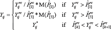
Y_{i j} = {\begin{matrix} Y_{i j}^{r c} / {\hat{P}}_{[1]}^{r c} * M ({\hat{P}}_{[1]}) & if & Y_{i j}^{r c} > {\hat{P}}_{[1]}^{r c} \\ Y_{i j}^{r c} / {\hat{P}}_{[5]}^{r c} * M ({\hat{P}}_{[5]}) & if & Y_{i j}^{r c} > {\hat{P}}_{[5]}^{r c} \\ Y_{i j}^{*} & if & {\hat{P}}_{[k]}^{r c} < Y_{i j}^{r c} < {\hat{P}}_{[k + 1]}^{r c} \end{matrix}

where M(·) is the median function $Y_{i j}^{*} = {(1 - q)}^{*} ((Y_{i j}^{r c} / {\hat{P}}_{[k]}^{r c} * M ({\hat{P}}_{[k]})) + q * ((Y_{i j}^{r c} / {\hat{P}}_{[k + 1]}^{r c} * M ({\hat{P}}_{[k + 1]}))$ and $q = ({\hat{P}}_{[k]}^{r c} - Y_{i j}^{r c}) / ({\hat{P}}_{[k]}^{r c} - {\hat{P}}_{[k + 1]}^{r c})$ .

Evaluation

We evaluated the single surface method with a set of 52 slides that were printed using Design I. Likewise, the multi-surface method was evaluated with a set of 276 arrays printed using Design II. We also used the Design II arrays to compare the single surface and multi-surface methods. Although there is not a gold standard in the data set, we can still adequately judge the effectiveness the spatial correction by comparing interslide reproducibility and spatial association.

Interslide Reproducibility

Interslide reproducibility was measured using the concordance correlation coefficient (CCC)²³ between the biological replicates on the array. The replicates were printed on different locations and sides (left vs. right), so replicate agreement is a reasonable assessment of the spatial correction. The CCC measures both correlation and deviation from the 45 degree identity line of the set of spots on the left side of the array and their corresponding replicates printed on the right side of the array. Like Pearson's correlation coefficient, the CCC is a number in the interval [–1,1] where a value of 1 represents perfect agreement.

Spatial Association

Spatial association was measured using Moran's I, a standard statistic in spatial data used to measure the strength of spatial correlation [2]. Moran's I is based on the definition of the “neighbors” of each spot. We defined the neighbor of a spot to be the 4 closest PC spots in all directions. Moran's I is a value in the interval [–1,1]. Under the null model, the expected value is –1/(n –1) where n is the number of spots. Values close to 1 indicate spatial correlation and slightly negative values close to zero indicate spatial independence.²⁴

Results and Discussion

Interslide Reproducibility

The mean CCC was higher for both Design I and Design II arrays after the surface correction was performed (Design I: no adjustment, 0.610; background, 0.850; surface, 0.886; Design II: no adjustment, 0.763; background, 0.865; surface, 0.892). Boxplots of CCC for both designs in Figure 6 show the variability of these measures.

Figure 6.

Concordance correlation coefficient (CCC) for the set of Design I (52 arrays) and Design II (276 arrays) slides before any adjustment and after background subtraction and surface corrections. Surface correction CCC is slightly higher than background subtraction alone.

For the Design I arrays, there was an increase of more than 0.025 in 27 of the slides, no substantial change in 24 slides, and a decrease of CCC in 1 slide. Furthermore, for the Design II arrays, single surface comparison with background subtraction alone showed that there was an increase of more than 0.025 of the CCC in 68 of the 276 arrays, no substantial change in 201 arrays, and a similar decrease in 7 of the arrays. When comparing the multi-surface technique with background subtraction alone, the CCC increased by more than 0.025 in 122 of the slides, had no substantial change in 145 slides, and decrease in 9 of the slides.

In summary, spatial correction with this data increases or does not change replicate agreement in 97% of the slides, with very dramatic improvement in some cases, for example, Arrays A and B from Figure 2. Furthermore, when replicated agreement is decreased, the slide generally had low variation to begin with (see Figure 8).

Figure 7.

Moran's I (a measure of spatial correlation) for the set of Design I (52 arrays) and Design II (276 arrays) slides before any adjustment and after background subtraction and surface corrections. There is substantially less spatial correlation after surface adjustments.

Figure 8.

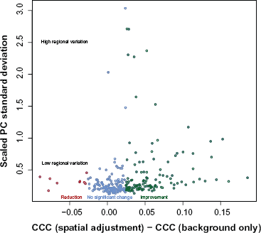
Surface adjustment is typically most benefical when high regional variation from non-print area staining is present. A reduction in interslide reproducibility is seen only for slides where spatial correction is not necessary (slides with low non-print area staining).

Spatial Association

Spatial association as measured by Moran's I indicated less spatial correlation in intensities after the surface correction. The mean Moran's I for Design I arrays was 0.705, 0.664, and 0.102 for no adjustment, background subtraction, and surface correction respectively. The means for Design II arrays were 0.371, 0.365, and –0.022. See Figure 7 for boxplots.

The Moran's I statistics was reduced (indicating less spatial correlation) for every slide from both the Design I and Design II arrays after surface correction.

Conclusion

In general, surface adjustment of intensities improves replicate agreement and better removes non-biological effects from the observed signal. There may be a concern that the surface adjustment does not uniformly improve interslide reproducibility. This method is useful when there is high regional variation from non-print area staining. Figure 8 shows that the slides for which the surface adjustment reduces replicate agreement are when the regional variation (measured as the scaled standard deviation of the positive controls) is low. There were some arrays with low regional variation that benefited from surface adjustment, therefore suggesting that the amount of regional variation is not always good indicator for when the method should not be used. We are currently researching criteria that will better indicate whether interslide reproducibility will suffer after surface adjustment.

Additional improvements in the surface adjustment can be attained when the positive control spots are printed in a dilution series. Often this is due to the fact that PC spots are saturated with protein when printed with full strength (Fig. 5). PC with a higher buffer to protein ratio will aid in surface correction when the full strength spots are saturated.

Overall, adjusting for regional variation from non-print area staining using positive controls improves interslide reproducibility and reduced spatial variability in RPPA. Background correction alone is not always sufficient to remove all the spatial variation that is present in RPPA data. The method that we have presented here using the positive control spots is both sensible and effective. We have developed a method that fits a 3-dimensional surface to positive controls and improves replicate concordance over typical background subtraction. When the positive control spots are printed in a dilution series, a set of nested surfaces built from different levels of positive control further improves replicate concordance. An important contribution of this method is that it allows valid use of data from a slide with regional non-print area staining that would otherwise have too much variation between replicates to be used. Application of the method saves from the need to restain slides and, thus, is an easy yet effective way to save resources.

Author Contributions

Conceived and designed the experiments: ESN, KAB, SMK. Analysed the data: ESN. Wrote the first draft of the manuscript: ESN, SMK. Contributed to the writing of the manuscript: ESN, KAB, SMK. Agree with manuscript results and conclusions: ESN, KAB, SMK. Jointly developed the structure and arguments for the paper: ESN, KAB, SMK. Made critical revisions and approved final version: ESN, KAB, SMK. All authors reviewed and approved of the final manuscript.

Funding

This work was supported by a Leukemia and Lymphoma Society translational research grant for SMK.

References

Nishizuka

, Charboneau

, Young

. Proteomic profling of the NCI-60 cancer cell lines using new high-density reverse-phase lysate microarrays. Proceedings of the National Academy of the Sciences of the United States of America. 2003; 100(24): 14229–34.

Paweletz

C.P.

, Charboneau

, Bichsel

V.E.

. Reverse phase protein microarrays which capture disease progression show activation of prosurvival pathways at the cancer invasion front. Oncogene. 2001; 20(16): 1981–9.

Grubb

R.L.

, Calvert

V.S.

, Wulkuhle

J.D.

. Signal pathway profiling of prostate cancer using reverse phase protein arrays. Proteomics. 2003; 3(11): 2142–6.

Nishizuka

, Chen

S.T.

, Gwadry

F.G.

. Diagnostic markers that distinguish colon and ovarian adenocarcinomas: Identification by genomic, proteomic, and tissue array profiling. Cancer Research. 2003; 63(17): 5243–50.

Gulmann

, Espina

III , Longo

E.P.

. Proteomic analysis of apoptotic pathways reveals prognostic factor in follicular lymphoma. Clinical Cancer Research. 2005; 11(16): 5847–55.

Akkiprik

, Nicorici

, Cogdell

. Dissection of signaling path-ways in fourteen breast cancer cell lines using reverse-phase protein lysate microarray. Technology in Cancer Research and Treatment. 2006; 5(6): 543–51.

Jiang

, Mircean

, Shmulevich

. Pathway alterations during glioma progression revealed by reverse phase protein lysate arrays. Proteomics. 2006; 6: 2964–71.

Kornblau

, Tibes

, Qiu

. Functional proteomic profiling of AML predicts response and survival. Blood. 2009; 113(1): 154–64.

Calvert

V.S.

, Collantes

, Elariny

. A systems biology approach to the pathogenesis of obesity-related nonalcoholic fatty liver disease using reverse phase protein microarrays for multiplexed cell signaling analysis. Hepatology. 2007; 46(1): 166–72.

10.

Chan

S.M.

, Ermann

, Su

, Fathman

C.G.

, Utz

P.J.

Protein microarrays for multiplex analysis of signal transduction pathways.

Nature Medicine. 2004; 10(12): 1390–6.

11.

, Ding

, Qian

. Predicting cancer drug response by proteomic profiling. Drug Discovery Today. 2006; 11(21/22): 1007–11.

12.

Mendes

K.N.

, Nicorici

, Cogdell

. Analysis of signaling pathways in 90 cancer cell lines by protein lysate array. Journal of Proteome Research. 2007; 6: 2753–67.

13.

Shankavaram

U.T.

, Reinhold

W.C.

, Nishizuka

. Transcript and protein expression profiles of the NCI-60 cancer cell panel: An integromic microarray study. Molecular Cancer Therapeutics. 2007; 6(3): 820–32.

14.

Wulfkuhle

J.D.

, Aquino

J.A.

, Calvert

V.S.

. Signal pathway profiling of ovarian cancer from human tissue specimens using reverse-phase protein microarrays. Proteomics. 2003; 3(11): 2085–90.

15.

Zha

, Raffeld

, Charboneau

. Similarities of prosurvival signals in Bcl-2-positive and Bcl-2-negative follicular lymphomas identified by reverse phase protein microarray. Laboratory Investigation. 2004; 84(2): 235–44.

16.

Tibes

, Qiu

, Lu

. Reverse phase protein array: Validation of a novel proteomic technology and utility for analysis of primary leukemia specimens and hematopoietic stem cells. Molecular Cancer Therapeutics. 2006; 5(10): 2512–21.

17.

Charboneau

, Scott

, Chen

. Utility of reverse phase protein arrays: Applications to signalling pathways and human body arrays. Brief Funct Genomic Proteomic. 2002; 1(3): 305–15.

18.

Espina

, Mehta

A.I.

, Winters

M.E.

. Protein microarrays: Molecular profiling technologies for clinical specimens. Proteomics. 2003; 3(11): 2091–100.

19.

Liotta

L.A.

, Espina

, Mehta

A.I.

. Protein microarrays: Meeting analytical challenges for clinical applications. Clinical Cancer Research. 2006; 12(15): 4583–9.

20.

Bland

M.J.

, Altman

D.G.

Statistical methods for assessing agreement between two methods of clinical measurement.

Lancet. 1986; 1(8476): 307–10.

21.

Kornblau

S.M.

, Coombes

K.R.

Protein Microarrays. vol. 785 of Methods in Molecular Biology. Humana Press, 2011; 10: 141–55.

22.

Wood

S.N.

Generalized Additive Models: An Introduction with R. Chapman and Hall, New York, 2006.

23.

Lin

L.I.K.

A concordance correlation coefficient to evaluate reproducibility.

Biometrics. 1989; 45: 255–68.

24.

Banerjee

, Carlin

, Gelfand

Hierarchical Modeling and Analysis for Spatial Data. Chapman and Hall, Boca Raton, 2004.

Surface Adjustment of Reverse Phase Protein Arrays using Positive Control Spots

Abstract

Keywords

Introduction

Methods

Data

Positive Controls

Surface Adjustment

Design I methods

Design II methods

Evaluation

Interslide Reproducibility

Spatial Association

Results and Discussion

Interslide Reproducibility

Spatial Association

Conclusion

Author Contributions

Funding

References