Sage Journals: Discover world-class research

Abstract

Motivated by the frustration of translation of research advances in the molecular and cellular biology of cancer into treatment, this study calls for cross-disciplinary efforts and proposes a methodology of incorporating drug pharmacology information into drug therapeutic response modeling using a computational systems biology approach. The objectives are two fold. The first one is to involve effective mathematical modeling in the drug development stage to incorporate preclinical and clinical data in order to decrease costs of drug development and increase pipeline productivity, since it is extremely expensive and difficult to get the optimal compromise of dosage and schedule through empirical testing. The second objective is to provide valuable suggestions to adjust individual drug dosing regimens to improve therapeutic effects considering most anticancer agents have wide inter-individual pharmacokinetic variability and a narrow therapeutic index. A dynamic hybrid systems model is proposed to study drug antitumor effect from the perspective of tumor growth dynamics, specifically the dosing and schedule of the periodic drug intake, and a drug's pharmacokinetics and pharmacodynamics information are linked together in the proposed model using a state-space approach. It is proved analytically that there exists an optimal drug dosage and interval administration point, and demonstrated through simulation study.

Keywords

drug effect drug efficacy region dosing regimens hybrid systems systems biology tumor growth

Introduction

The past three decades have seen spectacular advances in our understanding of the molecular and cellular biology of cancer. However, data suggest that the overall success rate for oncology products in clinical development is ~10%, and the cost of bringing a new drug to market is over US $1 billion.¹ Oncology drug development is such an expensive and prolonged process, typically, a new drug requiring on average 10 years.^2,3 New tools are needed to accelerate the drug discovery process and increase productivity.^4,5 While producing information both at the basic and clinical level is no longer the issue,⁶ the effective integration of data and knowledge from many disparate sources will be crucial to future cancer research.^7,8 Systems biology approaches promise to have a profound impact on medical practice by bringing together efforts from cross disciplinary scientists and permitting a comprehensive evaluation of underlying predisposition to disease, disease diagnosis, disease progression and disease treatment.^9–11

While providing the right drug for the right patient is very important, finding the right dose for each patient is also critical but tricky.¹² Finding a dose and dose range of a drug candidate that are both efficacious and safe is a fundamental objective through the drug discovery process.¹³ Dose finding happens throughout the long process of drug discovery, from non clinical development to multi-phase clinical trials. Even after the drug is approved and available on the market, new drug doses are still studied carefully and the level of investigation depends on responses observed from the general patient population. When necessary, dose adjustment based on post-marketing information is still a common practice. However, it is extremely expensive and difficult to get the optimal compromise of dosage and schedule through empirical testing. Modeling and simulation analysis, which can evolve and be continuously updated throughout different stages to incorporate relevant new data, will help to make crucial decisions earlier, with more certainty, and at lower cost, and hence can add value in all stages of drug development.^5,14

The complexity of cancer itself and the heterogeneity of therapeutic responses may make dosing study more complicated. For example, most anticancer agents have wide inter-individual pharmacokinetic (PK) variability and a narrow therapeutic index.¹⁵ Recent works have shown that many patients who are currently being treated with 5-fluorouracil (5-FU) are not being given the appropriate doses to achieve optimal plasma concentration. Of note, only 20%–30% of patients are treated in the appropriate dose range, approximately 40%–60% of patients are being underdosed, and 10%–20% of patients are overdosed.¹⁶ Traditionally, the standard approach for calculating 5-FU drug dosage, as with many anticancer agents, has been done by normalizing dose to body surface area (BSA), which is calculated from the height and weight of the patient;¹⁶ however, studies have shown that this is inadequate.¹⁷ For example, dosing based on BSA is associated with considerable variability in plasma 5-FU levels by as much as 100-fold,^15,17 and such variability is a major contributor to toxicity and treatment failure.¹⁶ Since there are many factors collaboratively affecting drug effect variability,¹⁸ a general approach is needed to facilitate quantitative thinking to drug administration regimens. Drug dosing regimens could be tailored to each individual patient based on feedback information from the treatment. One challenge of such modeling is how to link relevant biomarkers¹⁹ or surrogate endpoints to treatment outcome as feedback information in order to give valuable dosing suggestions.

Traditional design of the dosing regimen based on achieving some desired target goal such as relatively constant serum concentration may be far from optimal owing to the underlying dynamic biological networks. For example, Shah and co-workers²⁰ demonstrate that the BCR-ABL inhibitor dasatinib, which has greater potency and a short half-life, can achieve deep clinical remission in CML patients by achieving transient potent BCR-ABL inhibition, while traditional approved tyrosine kinase inhibitors usually have prolonged half lives that result in continuous target inhibition. A similar study of whether short pulses of higher dose or persistent dosing with lower doses have the most favorable outcomes has been carried out by Amin and co-workers²¹ in the setup of inactivation of HER2-HER3 signaling. For best results, models should be selected based on the underlying mechanism of drug action. For example, detailed dynamic signal transduction models are needed to accommodate target-receptor interaction and feedback loops for analyzing dosing effect in the above examples.

Computational systems biology is emerging as a valuable tool in therapeutics to address these challenges.^10,22–25 This approach provides functional understanding of disease-drug interaction and marks a shift from the traditional “black-box” approach. In this study, a general methodology incorporating dynamic drug pharmacology information into drug therapeutic response modeling using computational systems biology is proposed. The process begins with building a quantitative model of a biological system. Then, by incorporating related pharmacology information relevant to the target system, a new computational model under drug perturbation can be built. We believe that with the help from the theoretical modeling proposed in this study and through an iterative process with experimentalists to refine the model, the proposed methodology has the potential to supply better recommendations for dosage and frequency.

Modeling

A good model should be based on a sound understanding of the biological problem, hold a realistic mathematical representation of the biological phenomena, and possess a tractable solution.²⁶ A biological interpretation of the deductions resulting from such a model can yield non-intuitive insights, as well as provide a predictive framework,¹⁰ a vital issue in cancer treatment. In recent years it has become clear that carcinogenesis is a complex process, both at the molecular and cellular levels.^25,27 Modeling biological systems to develop computer models of disease that can be used to understand disease mechanisms and to test in silico approaches for treating disease is a key issue in moving forward. Recent mathematical advances have made it more feasible to model cancer from a mathematical viewpoint. There are numerous works modeling cancer at multiple levels and scales, ranging from molecules to cells to tissues.^7,28 For example, multi-scale models have been developed that can capture interactions across different spatial and temporal scales.⁸ A number of researchers have recommended hybrid or hierarchical systems to combine the strengths of both discrete and continuous approaches.^8,29,30

Biological systems are naturally nonlinear; however, purely nonlinear continuous models of biological systems can be too large and complex for simulation and analysis. On the other hand, a linear continuous model or a fully discrete approximation of the model can sometimes lose crucial and pertinent information.³¹ Hybrid systems³² provide a rigorous foundation for modeling biological systems at desired levels of abstraction, approximation, and simplifications.³³ For example, systems that exhibit multi-scale dynamics can be simplified by replacing certain slowly changing variables by their piecewise constant approximations. Additionally, sigmoidal nonlinearities are commonly observed in biology and the corresponding models often use sigmoidal functions. These can be approximated by discrete transitions between piecewise-linear regions. In some instances, nondeterministic upper and lower bounds are more useful than deterministic approximations because they capture all critical behavior of the system.^33–35 The hybrid systems model encapsulates a broad space of models and systems. For example, the Lac operon system has been well studied both experimentally and using continuous models.^36,37 A hybrid model and use of a reachability algorithm were validated by comparison with experimental data and continuous models.³⁸ Other biological hybrid systems analyzed in similar ways include the Delta-Notch decision process,^39,40 genetic regulatory networks of carbon starvation,⁴¹ nutritional stress response⁴² in E. coli, and our previous work on drug effect modeling under genetic regulatory networks.⁴³ In this study, we adopt hybrid systems models to accommodate the hybrid nature of disease progression and therapeutic responses. Specifically, a tumor growth model under drug perturbation is studied to demonstrate how to integrate diverse data and ultimately predict outcomes for clinical purposes.

Tumor growth model using hybrid systems

Cancer research has been a fertile ground for mathematical modeling.⁴⁴ A number of mathematical tumor growth models have been reported in the literature, reflecting different paradigms. Empirical models use mathematical equations to describe the tumor growth curve without in-depth mechanistic description of the underlying physiological processes. Initially, models were used to conceptualize the simple exponential growth of solid tumors.^45–47 Subsequently, sigmoidal functions such as logistic, Verhulst, Gompertz, and von Bertalanffy were used for the description of reduced growth in the later stages as the tumor cells outgrew their blood supply, producing central necrosis.^48–51 A drawback of this model class is that it is not straightforward to predict modification of the growth curve under drug perturbation. Functional models, conversely, are based on mechanistic descriptions of biological processes underlying tumor growth. Such models require a set of assumptions involving cell cycle kinetics (proliferating vs. quiescent cells) and biochemical processes, such as those related to antiangiogenic and/or immunological responses.^52,53 Owing to the biological complexity they try to capture, these models have a much larger number of parameters compared with the empirical models. Hence, in addition to the standard tumor growth measurements, further data are needed, such as flow cytometry analysis and measurements of biochemical and immunological markers, to avoid identification problems due to the over parametrization.⁵³ The situation becomes even more complex when the effect of treatment with an anticancer drug is considered on account of the incomplete knowledge of the mode of action in vivo.

It is important to realize that all models have limitations, including those in oncology: simple models may produce insights and describe existing data, but they risk oversimplification and oversight of critical variables; on the other hand, it is generally difficult to fit functional models versus experimental data since over parametrization can be avoided only if further “microscopic” observations are available. Hence, it is a challenge to achieve a correct balance between empirical and functional models. In this paper, we adopt a model that is a compromise between empirical and mechanism-based approaches.^54,55 The model is based on a system of ordinary deferential equations that link the dosing regimen of a compound to the tumor growth in xenograft mice, with tumor growth in untreated animals being described by exponential growth followed by a linear growth phase. In treated animals, the tumor growth rate decreases proportionally to both drug concentration and the number of proliferating tumor cells. It relies on a few identifiable parameters, the estimation of which requires only the data typically available in the preclinical setting. There are two parameters related to drug effect: c(t), the drug concentration, and k₂ a constant measuring drug potency.⁵⁵ In their later study,⁵⁶ good correlation was achieved with a novel approach proposed to predict the expected active dose in humans from the studies mentioned above.^54,55

Although modeling in tumor growth has attracted a lot of attention, most of the aforementioned efforts have not explored the impact of drug effects. There is some work assuming the system is at steady state, which means that the concentrations of active drugs at the active site are constant. In some drug effect models,^55,57,58 drug effect is assumed to be related to drug concentration and number of tumor cells; however, if we would like to compare drug effects for different dosing regimens to consider issues as whether we give patient frequent small or infrequent large drug dosage given fixed total drug intake, more realistic and dynamic drug effect models are needed. This study proposes a model dynamically linking disease progression, in which hybrid systems are adopted to accommodate disease progression and therapeutic responses. Specifically, we adapt the tumor growth model proposed in⁵⁴ to hybrid systems model to accommodate the tumor growth dynamics in different stages and augment it with a drug effect model related to PK and pharmacodynamics (PD). In this proposed framework, PK and PD are linked by a state-space approach, where drug concentration will fluctuate between dosages and drug efficacy will change with drug concentration. Our main aim is to model drug effect on tumor growth for different treatment dosing regimens given related pharmacology information.

Unperturbed growth model (without drug treatment)

Following the same biology setup as Magni et al,⁵⁴ unperturbed and perturbed growth models are formulated to model tumor growth dynamics without treatment and with treatment, respectively. Tumor growth is modeled by an exponential growth phase followed by a linear growth phase for the unperturbed growth model. A hybrid systems model is proposed to accommodate tumor growth dynamics in different stages. It takes the form

{\dot{w}}_{u} = β_{1} w_{u} s^{-} (w_{u}, θ_{w}) + β_{0} s^{+} (w_{u}, θ_{w}),

(1)

where w_u denotes unperturbed tumor weight, β₁ and β₀ are parameters characterizing the rates of exponential and linear growth. s⁺(·) is the unit step function defined by

s^{+} (x, θ) = {\begin{matrix} 0 & x < θ \\ 1 & x \geq θ \end{matrix},

(2)

s^−-(·) = 1 – s⁺(·), and θ_w is the corresponding threshold value at which tumor growth switches from exponential to linear growth. To assure the continuity of derivatives in Equation (1) at θ_w, θ_w = β₀/β₁ can be derived. Given current progress in tumor growth modeling, the tumor growth characteristics might be quite different in different situations. The proposed model based on hybrid systems can be extended to accommodate more complicated cases, such as more growth stages with different growth rates.

Perturbed growth model (with drug treatment)

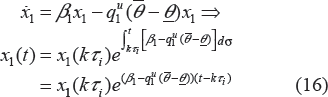
All the tumor cells are assumed to be proliferating in the unperturbed model. With drug treatment, it is assumed that cells affected by drug action stop proliferating and pass through different stages characterized by progressive degrees of damage and eventually they die.⁵⁵ A transit compartment model is used for the cells’ progression to death under drug treatment:

{\dot{x}}_{1} = β_{1} x_{1} s^{-} (w_{p}, θ_{w}) + β_{0} \frac{x_{1}}{w_{p}} s^{+} (w_{p}, θ_{w}) - γ_{1}^{u} x_{1}

(3)

{\dot{x}}_{2} = γ_{1}^{u} x_{1} - k_{1} x_{2}

(4)

{\dot{x}}_{3} = k_{1} (x_{2} - x_{3})

(5)

⋮

(6)

{\dot{x}}_{n} = k_{1} (x_{n - 1} - x_{n})

(7)

w_{p} = \sum_{i = 1}^{n} x_{i}

(8)

x_{1} (0) = w_{0}

(9)

x_{2} (0) = x_{3} (0) = \dots x_{n} (0) = 0

(10)

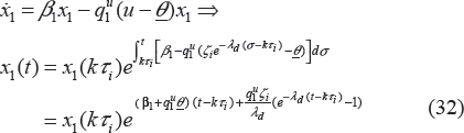
where x₁ indicates the portion of proliferating cells within the total tumor weight w_p with drug treatment. x₁(t) will go through exponential and then linear growth similar to the unperturbed tumor model, where β₁ and β₀ denote the respective growth parameters. In these equations, w_p is the total tumor weight, represented by the sum of cells in the various stages, and w₀ is the tumor weight at the inoculation time (t = 0). Since not all cells are proliferating, the linear growth rate is slowed down by the ratio of the proliferating cells over the total tumor cells x₁/w_p. The model assumes that the drug elicits its effect related to the number, x₁, of proliferating cells and $γ_{1}^{u}$ . $γ_{1}^{u}$ is the drug effect coefficient and will be defined in the next section (drug treatment model), which is closely related to drug efficacy (PD) and fluctuates based on changes of drug concentration (PK). The damaged tumor cells proceed through progressive degrees of damage through n different stages with rate constant k₁. The term k₁x_n represents the weight of cells that die in each unit of time.

Drug treatment model

The basis of clinical pharmacology is the fact that the intensities of many pharmacological effects are functions of the amount of drug in the body and, more specifically, the concentration of drug at the effect site.⁵⁹ For a long time, PK and PD had been considered as separate disciplines; however, the information provided by these disciplines is limited if regarded in isolation. On one hand, PK is characterized as what the body does to the drug, and it denotes the concentration-time course of drugs in different body fluids. On the other hand, PD is assessed as what the drug does to the body, and it characterizes the intensity of effects resulting from certain drug concentrations at the assumed effect site. In order to describe the time course of drug effect in response to different dosing regimens, the integrated PK/PD model is indispensable, which builds the bridge between these two classical disciplines of pharmacology.⁶⁰ Following each dosing regimen, instead of a two dimensional dose-concentration (PK) and concentration-effect (PD) relationship, our proposed approach enables a description of a three dimensional dose-concentration-effect relationship. Specifically, PK and PD are linked through a state-space approach to facilitate the description and prediction of the time course of drug effects resulting from different drug administration regimens.

PK/PD modeling is an active research area in pharmacology^5,59 Application of such concepts has been identified as potentially beneficial in all phases of preclinical and clinical drug development.^61,62 This work is our first attempt in the direction of quantitative drug effect modeling. Although we make some assumptions about concentration-effect and dose-concentration curves in this paper, the methodology proposed is flexible enough such that many specific PK/PD data can be accommodated in the proposed framework. If the mathematical formulation becomes too complicated and theoretical analysis is not possible, an extensive simulation study can be carried out for available PK/PD data.

Periodic drug intake: pharmacokinetics (PK) model

We consider a periodic drug intake scenario. One could use a detailed theoretical or empirical pharmacokinetic description of time dependent drug concentration at the site of action in a simulation study. We prefer to keep the model mathematically tractable so that we can perform a strict theoretical analysis and thereby gain insights. Thus, we assume the concentration has exponential decay. 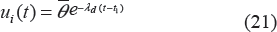Since we are using hybrid systems, the PK model can be extended to include more complicated cases, such as the case where the drug concentration will first exponentially increase, then slowly change (equilibrium), and then exponentially decrease.⁶³ The model used for drug intake and concentration levels is illustrated in Figure 1. We denote the period of drug intake for the two cases as τ₁ and τ₂, respectively. Without loss of generality, it is assumed that τ₁ = Mτ₂, where M > 1 is an integer. It is also assumed that u₁(kτ₁) = ζ₁ = Mu₂(lτ₂) = Mζ₂, where k and l are non-negative integers, and ζ₁ and ζ₂ are dosages in cases 1 and 2, respectively. This means that, in the long run, the patient takes the same total drug amount in both cases. It is assumed that the concentration level of the drug at the effect site follows exponential decay during each period, ie, $u_{i} (t) = ζ_{i} e^{- λ_{d} (t - k τ_{i})}$ , where kτ_i ≤ t ≤ (k + 1)τ_i and λ_d is the degradation factor. Note that Figure 1 does not show the case where there is “leftover” from the previous dosage when the patient is taking the current dosage.

Figure 1.

The concentration level of drug under periodic drug intake. Two cases are shown: (1) large dose with longer period; (2) small dose with shorter period.

Drug efficacy and potency: pharmacodynamics (PD) model

The PK model provides the concentration time course resulting from the administered dose and the continuous description of concentration will serve as input function for the PD model, which relates the concentration to the observed effect. Generally, the magnitude of pharmacological effect increases monotonically with increased dose, eventually reaching a plateau level where further increases in dose have little additional effect.¹³ The classic and most commonly used concentration-effect model is the Hill equation,⁶⁴ also called the sigmoidal E_max model⁶⁵ or logistic model.⁶⁶ The relationship between the concentration of the drug candidate and its effect is most often nonlinear. In some cases, the curve even looks like a “roller coaster”, which is referred to as the “double Hill Model”.⁶⁷ One common method is to replace certain slowly changing variables by their piecewise linear approximation. In this study, we use hybrid systems to approximate the sigmoidal E_max PD model (see Fig. 3). The E_max model has the general form:

E = \frac{E_{\max} C^{m}}{E C_{50}^{m} + C^{m}},

(11)

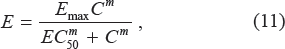
where E_max is the maximum effect, C is the concentration, EC₅₀ is the concentration necessary to produce 50% of E_max, and m represents a sigmoidity factor or steepness of the curve.

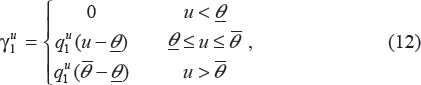
We assume a threshold of concentration below which the drug candidate is ineffective (such dose is often called the minimum effective dose (MinED)). We assume another threshold called the maximum effective dose (MaxED), above which there is no clinically significant increase in pharmacological effect. We use a linear curve to approximate the concentration-effect curve between MinED and MaxED. We assume that the drug effect coefficient $γ_{1}^{u}$ is related to the concentration u through a sigmoid function and can be approximated by the curve shown in Figure 2. The corresponding relationship can be expressed as

γ_{1}^{u} = {\begin{matrix} 0 & u < \underline{θ} \\ q_{1}^{u} (u - \underline{θ}) & \underline{θ} \leq u \leq \bar{θ} \\ q_{1}^{u} (\bar{θ} - \underline{θ}) & u > \bar{θ} \end{matrix},

(12)

Figure 2.

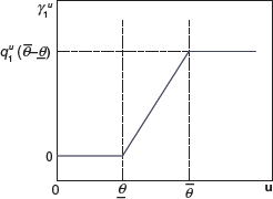
The Concentration-effect curve.

where $q_{1}^{u}$ is the ratio between the drug effect coefficient and the drug concentration (in the linear range). This reflects the fact that the drug only starts to take effect when its concentration level is above a lower threshold ( $\underline{θ}$ , corresponding to MinED) and its effect saturates when its concentration level exceeds an upper threshold ( $\underline{θ}$ , corresponding to MaxED). Note that the sigmoidal E_max model can be well approximated by the proposed PD model. By taking the derivative of E with respect to C and evaluating it at EC₅₀, we obtain the slope as $q_{1}^{u} = m E_{\max} / 4 E C_{50}$ . The upper and lower bound should satisfy $q_{1}^{u} = (\bar{θ} - \underline{θ}) = E_{\max}$ . An example of the sigmoidal E_max model when m = 4 and our proposed PD model are plotted together in Figure 3, where it is observed that our proposed model closely resembles the sigmoidal E_max model. Furthermore, by tuning the parameters in the proposed model, we may approximate many different types of PD models in the literature.

Figure 3.

Sigmoidal E_max model (m = 4), and approximation by our PD model.

Drug effect analysis

Based on the proposed perturbed growth model (Eqs. (3) to (7)), the drug effect is related to the number of proliferating tumor cells x₁ and drug effect coefficient $γ_{1}^{u}$ . Since the changes of the number of the proliferating cells dominate the changes of all the cells under drug treatment (please refer to Appendix A for proof), we will study the drug effect on the number of proliferating cells in our analytical study. We first decouple the growth phase into two stages based on tumor weight.⁵⁵ In the first stage of the tumor growth, when tumor weight x₁ < θ_w, the model with drug treatment is given by

{\dot{x}}_{1} = β_{1} x_{1} - γ_{1}^{u} x_{1}

(13)

where $γ_{1}^{u}$ is defined by Eq. (12). Based on the preceding assumptions, the hybrid systems model can be updated by incorporating Figures 1 and 2 into Eq. 13. We consider a realistic setting where a patient takes the drug periodically. For each period kτ_i ≤ t ≤ (k + 1)τ_i, i = 1, 2, …, representing different dosage and schedule arrangements,

{\dot{x}}_{1} = β_{1} x_{1} - q_{1}^{u} (u_{1} - \underline{θ}) s^{+} (u_{i}, \bar{θ}) x_{1} - q_{1}^{u} (\bar{θ} - \underline{θ}) s^{+} (u_{i}, \bar{θ}) x_{1}

(14)

u_{i} (t) = ζ_{i} e^{- λ_{d} (t - k τ_{i})}

(15)

where u_i(t) is the drug concentration level at the assumed effect site.

State-space analysis

In our proposed model, there are both continuous quantitative changes (eg, the drug concentration level) and discrete transitions (eg, PD model). As is common in hybrid systems, there are both continuous and discrete states. The entire state space may be divided into different domains according to the value of the discrete state. When the quantitative change of the continuous state meets certain criteria, it will cause a discrete transition from one domain to another. Specifically, after each drug intake, the drug concentration at the effect site is dynamically changing following the PK model, with the changing concentration falling into different ranges (domains). The tumor growth dynamics will change according to different PD model at each domain. A state space and trajectory plot of the state of the proliferating tumor growth and drug concentration level under periodic drug intake are illustrated in Figure 4. There are five domains in the state space, with D₁ D₃, D₅ not being transient.

Figure 4.

The trajectory of the state (tumor weight growth and drug concentration level) under periodic drug intake $ζ_{i} > \bar{θ}$ . δ is a very small positive number.

The figure shows the case when the drug is effective and the initial drug concentration level is larger than the upper threshold $\bar{θ}$ (that means the state trajectory starts from Domain D₅) and the sample trajectory of the state corresponds to two periods of drug intake. We observe that, when the state transits in each period under periodic drug intake, it may pass through different domains (depending on the drug concentration decay along time). When the drug concentration is higher than $\underline{θ}$ (MinED), the drug has an anti-tumor effect. The tumor weight may decrease (the tumor growth level is pushed to the left) depending on drug efficacy and concentration during the transit time through domains D₅ and D₃; however, the tumor will grow during the transit time through domain D₁, where the drug is not effective because its concentration is below MinED. In order for the drug to be effective, the push to left side should be stronger than the push to the right side. This means that we should have x₁((k + 1)τ) ≤ x₁ (kτ), so that after each treatment period the number, x₁, proliferating tumor cells will decrease.

Depending on the initial drug intake, the state trajectory may start from different domains. For example, if the initial conditions are x₁ = x₁(kτ_i) and u_i = ζ_i > $u_{i} = ζ_{i} > \bar{θ}$ (as in Fig. 4), then the state trajectory starts from domain D₅ (Case 1). If the initial condition is $\underline{θ} < u_{i} = ζ_{i} < \bar{θ}$ , then the state trajectory starts from domain D₃ (Case 2). The state trajectory starting from D₁ corresponds to the case where the drug concentration is too low to be effective, and therefore has no therapeutic effect.

Case 1: state trajectory starts from domain D₅

We define t₁ as the traveling time from the initial condition to the boundary between D₅ and D₃, and t₂ as the traveling time from the initial condition to the boundary between D₃ and D₁. The traveling time within D₃ is therefore t₂ – t₁. Since we are considering the case that state trajectory starts from domain D₅, the initial conditions are x₁ = x₁(kτ_i) and $u_{i} = ζ_{i} > \bar{θ}$ . For kτ_i ≤ t ≤(k + 1)tau;_i, i = 1,2., the corresponding equations and solutions in each domain are given by – D₅ (from time kτ_i to t₁, ie, kτ_i ≤ t ≤ t₁):

\begin{matrix} {\dot{x}}_{1} = β_{1} x_{1} - q_{1}^{u} (\bar{θ} - \underline{θ}) x_{1} \Rightarrow \\ x_{1} (t) = x_{1} (k τ_{i}) e^{\int_{k τ_{i}}^{t} [β_{1} - q_{1}^{u} (\bar{θ} - \bar{θ})] d σ} \\ = x_{1} (k τ_{i}) e^{(β_{1} - q_{1}^{u} (\bar{θ} - \underline{θ}) (t - k τ_{i}))} \end{matrix}

(16)

u_{i} (t) = ζ_{i} e^{- λ_{d} (t - k τ_{i})}

(17)

In order to reduce x₁, we need

(β_{1} - q_{1}^{u} (\bar{θ} - \underline{θ})) (t - k τ_{i}) < 0

(18)

this implies

β_{1} < q_{1}^{u} (\bar{θ} - \underline{θ})

(19)

–D₃ (from time t₁ to t₂, ie, t₁ ≤ t ≤ t₂):

\begin{matrix} {\dot{x}}_{1} = β_{1} x_{1} - q_{1}^{u} (u - \underline{θ}) x_{1} \Rightarrow \\ x_{1} (t) = x_{1} (t_{1}) e^{\int_{t_{1}}^{t} [β_{1} - q_{1}^{u} ({\bar{θ}}_{e} - λ_{d} (σ - t_{1}) - \underline{θ})]} \\ = x_{1} (t_{1}) e^{(β_{1} + q_{1}^{u} \underline{θ}) (t - t_{1}) + \frac{q_{1}^{u} \bar{θ}}{λ_{d}} (e^{- λ_{d} (t - t_{1})} - 1)} \end{matrix}

(20)

u_{i} (t) = \bar{θ} e^{- λ_{d} (t - t_{1})}

(21)

In order to reduce x₁ we need

(β_{1} - q_{1}^{u} \underline{θ}) (t - t_{1}) + \frac{q_{1}^{u} \bar{θ}}{λ_{d}} (e^{- λ_{d} (t - t_{1})} - 1) < 0

(22)

–D₁ (from time t₂ to (k + 1)τ_i, ie, t₂ ≤ t ≤ (k + 1)τ_i):

{\dot{x}}_{1} = β_{1} x_{1}, \Rightarrow x_{1} (t) = x_{1} (t_{2}) e^{β_{1} (t - t_{2})}

(23)

u_{i} (t) = \underline{θ} e^{- λ_{d} (t - t_{2})}

(24)

Since the drug dosage is below the effective level ( $\bar{θ}$ ), the drug is not effective on the tumor, as expected.

For the drug to be effective, both the inequalities (22) and (19) must be satisfied; however, they are just loose bounds. We could deduce the necessary and sufficient condition for the effectiveness of the drug by expressing the inequality x₁((k + 1)τ) ≤ x₁(kτ) in terms of the dose period τ and unit dose ζ, so that after each treatment period the number of proliferating tumor cells x₁ will decrease. When the initial conditions are x₁ = x₁(kτ_i) and $u_{i} = ζ_{i} > \bar{θ}$ , the equations governing the state trajectory from time kτ_i to time (k + 1)τ_i are given by

x_{1} (t_{1}) = x_{1} (k τ_{i}) e^{(β_{1} - q_{1}^{u} (\bar{θ} - \underline{θ}) (t_{1} - k τ_{i})}

(25)

x_{1} (t_{2}) = x_{1} (t_{1}) e^{(β_{1} - q_{1}^{u} \underline{θ}) (t_{2} - t_{1}) + \frac{q_{1}^{u} \bar{θ}}{λ_{d}} (e^{- λ_{d} (t_{2} - t_{1})} - 1)}

(26)

x_{1} ((k + 1) τ_{t}) = x_{1} (t_{2}) e^{β_{1} ((k + 1) τ_{i} - t_{2})}

(27)

\bar{θ} = ζ_{i} e^{- λ_{d} (t_{1} - k τ_{i})}

(28)

\underline{θ} = \bar{θ} e^{- λ_{d} (t_{2} - t_{1})}

(29)

and can be simplified to

x_{1} ((k + 1) τ_{i}) = x_{1} (k τ_{i}) e^{Ψ}

(30)

Ψ = β_{1} τ_{i} + \frac{q_{1}^{u}}{λ_{d}} [\bar{θ} l n \bar{θ} - \underline{θ} l n \underline{θ} - (1 + l n ζ_{i}) (\bar{θ} - \underline{θ})]

(31)

For the drug to be effective, we need Ψ < 0, so that the number of proliferating tumor cells x₁ will decrease following each period of drug intake.

Case 2: state trajectory starts from domain D₃

When the drug dosage is below $\bar{θ}$ but is above $\underline{θ}$ the initial conditions are given by x₁ = x₁(kτ) and $u_{i} = \underline{θ} < ζ_{i} < \bar{θ}$ . In this case, for kτ_i ≤ t ≤(k + 1)τ_i, i = 1, 2., the corresponding equations and solutions of the domains are given by –D₃ (from time kτ_i to t₂):

\begin{matrix} {\dot{x}}_{1} = β_{1} x_{1} - q_{1}^{u} (u - \underline{θ}) x_{1} \Rightarrow \\ x_{1} (t) = x_{1} (k τ_{i}) e^{\int_{k τ_{i}}^{t} [β_{1} - q_{1}^{u} (ζ_{i} e^{- λ_{d} (σ - k τ_{i})} - \underline{θ}] d σ} \\ = x_{1} (k τ_{i}) e^{(β_{1} + q_{1}^{u} \underline{θ}) (t - k τ_{i}) + \frac{q_{1}^{u} ζ_{i}}{λ_{d}} (e^{- λ_{d} (t - k τ_{i})} -)} \end{matrix}

(32)

u_{i} (t) = ζ_{i} e^{- λ_{d} (t - k τ_{i})}

(33)

–D₁ (from time t₂ to (k + 1)τ_i):

{\dot{x}}_{1} = β_{1} x_{1}, \Rightarrow x_{1} = x_{1} (t_{2}) e^{β_{1} (t - t_{2})}

(34)

u_{i} (t) = \underline{θ} e^{- λ_{d} (t - t_{2})}

(35)

The equations governing the state trajectory from time kτ_i to time (k + 1) τ_i are given by

x_{1} (t_{2}) = x_{1} (k τ_{i}) e^{(β_{1} - q_{1}^{u} \underline{θ}) (t - k τ_{i}) + \frac{q_{1}^{u} ζ_{i}}{λ_{d}} (e^{- λ_{d} (t - k τ_{i}) - 1)}}

(36)

x_{1} ((k + 1) τ_{i}) = x_{1} (t_{2}) e^{β_{1} ((k + 1) τ_{i} - t_{2})}

(37)

\underline{θ} = ζ_{i} e^{- λ_{d} (t_{2} - k τ_{i})}

(38)

This can be simplified to

x_{1} ((k + 1) τ_{i}) = x_{1} (k τ_{i}) e^{Ψ}

(39)

Ψ = β_{1} τ_{i} + \frac{q_{1}^{u}}{λ_{d}} [ζ_{i} l n ζ_{i} - \underline{θ} l n \underline{θ} - (1 + l n ζ_{i}) (ζ_{i} - \underline{θ})]

(40)

For the drug to be effective, we need Ψ < 0, so that the number of proliferating tumor cells will decrease following each period of drug intake.

Tumor growth minimization

We have proved mathematically that the reduction of the number of proliferating tumor cells, defined as x₁((k + 1)τ_i) – x₁ (kτ_i), is a strictly convex function⁶⁸ of time interval τ_i. The detailed proof is given in the Appendix A. This implies that the function of tumor size reduction, which should be negative for a successful treatment, has a “U” shape and has a unique global minimum point,⁶⁸ where x₁((k + 1)τ_i)–x₁ (kτ_i) < 0 is the smallest that corresponds to the maximum reduction in tumor size (where |x₁((k + 1)τ_i)–x₁(kτ_i)| is the largest).

Results

In order to validate the analytical results on drug effect for different dosing regimens, we firstly perform numerical simulations using predefined parameters to validate the analytical results. Then we proceed with parameter estimation on synthetic data sets generated based on the experimental study.^54,55 This second step is critical to facilitate the use of hybrid mathematical model to biologist. We also demonstrate that similar conclusion on drug efficacy region can be drawn based on the synthetic data sets generated using the parameters from real experiments.

Simulations using predefined parameters

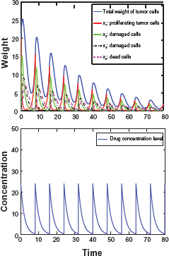
In order to validate the analytical results on drug effect, we firstly perform numerical simulations using MATLAB/SIMULINK, based on the detailed transit compartment model presented from Eqs. (3) to (7). The cells affected by drug action stop proliferating and pass through four different stages, x₁, x₂, x₃, and x₄, characterized by progressive degrees of damage, where x₁ indicates the portion of proliferating cells and w_p is the total tumor weight. Specifically, the parameters in the simulation are β₁ = 1.0, β₀ = 0.2, k₁ = 1.0, θ_w = 40. For the PD model, we follow Eq. (12) and set the parameters as $q_{1}^{u} = 0.21$ , $\underline{θ} = 1.0$ , and $\bar{θ} = 21$ For the PK model, we consider periodic drug intake and the drug concentration level follows an exponential decay during each period, as illustrated in Figure 1. The decay rate is λ_d = 0.5.

Observation 1: To compare the effect of different dosages and frequencies given a certain total drug intake, we define the density of drug intake as $α = ζ_{i} / τ_{i}$ , where ζ is the dosage and τ is the dosing period. In practice, α is related to drug toxicity level. The time course of responses of the tumor weight change (including the 4 different stages based on damages) under three different dosing regimens (all with total drug intake α = 3.0) are compared: small frequent dosage (dosage = 15 and period (τ) = 5), medium and less frequent dosage (dosage = 24, and period (τ) = 8), and large infrequent dosage (dosage = 45 and period (τ) = 15). These are shown in Figures 5–7, respectively.

Figure 5.

τ = 5, ζ = 15, Ψ = 0.7.

Figure 6.

τ = 8, ζ = 24, Ψ = –0.24.

Figure 7.

τ = 15, ζ = 45, Ψ = 1.5.

Figures 5–7 show the responses of tumor under three dosing regimens (all with same total drug intake α = 3.0). The left figure (Fig. 5) corresponds to the small frequent dosing, the right figure (Fig. 7) corresponds to the large infrequent dosing, and the case of intermediate dosing in between (Fig. 6). Other parameter setting for the above figures: β₁ = 1.0, β₀ = 0.2, k₁ = 1.0, θ _w = 40, $q_{1}^{u} = 0.21$ , $\underline{θ} = 1.0$ , $\bar{θ} = 21$ , and λ_d = 0.5.

We observe that the changes of total tumor weight w_p follow similar patterns with the changes of the number of proliferating cells x₁, which confirms our theoretical analysis. Moreover, the results clearly show that dosing regimens play a critical role in disease treatment, even when the total drug in take remains the same. Both the small frequent dosing (Fig. 5) and large in frequent dosing case (Fig. 7) do not reduce the tumor size effectively. Only in the case with moderate dosage and interval (Fig. 6), are both the number of proliferating cells and the total tumor weight reduced effectively. At the same time, the results demonstrate what is predicted in the analytical results: we need Ψ < 0 so that the tumor will degrade following each period of drug intake.

Observation 2: To further verify that the change of tumor weight between treatments, Δx₁ = x₁((k + 1) τ) – x₁(kτ), is a strictly convex function of time interval, we plot the percentage of tumor weight change versus dosing period τ in Figure 8 for different total drug intakes with α = 2.8, 2.9, 3.0, 3.1, 3.2. For each curve with fixed total drug intake, it can be seen that Δx₁ is indeed convex, and an optimal choice of drug administration can be made based on the point of maximum tumor reduction. There exist some “sweet spots” (defined as “drug efficacy regions”) of drug administration that will satisfy the condition Ψ < 0. The three special dosing cases (Figs. 5–7, with α = 3.0) can be tested in the curve and it is easily confirmed that only the moderate dosage and interval case with τ = 8 falls into the drug efficacy region. Furthermore, Figure 8 illustrates the tradeoff between efficacy and toxicity. When the total drug intake α increases, the drug efficacy region gets larger accordingly. At another extreme, the drug efficacy region may not exist when α gets too small.

Figure 8.

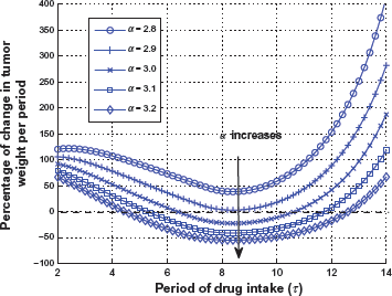
The percentage of tumor weight change change vs. τand total drug intake α, where decay rate λ_d is same).

Observation 3: There are many factors that affect drug response, inter-individual PK variability being one of them. Thus, it is important to check how different PK parameters change drug effect. In this study, we plot the percentage of tumor weight change versus τ for different PK decay rates (λ_d = 0.42, 0.44, 0.46, 0.48, 0.5) in Figure 9. It is observed that the effect of PK (specifically, the decay rate λ_d) on tumor reduction is significant. When the drug decay is slow, say λ_d = 0.42, the tumor weight will decrease much faster than when drug decay is fast, say λ_d = 0.5. This confirms our hypothesis that the drug effect is closely related to the PK parameters, which is one reason for the heterogeneity of therapeutic responses. Hence, if we could estimate inter-individual PK variability based on accurate measurement and interpretation of drug concentration in biological fluids and perform corresponding therapy assessment to model disease progression, then it is possible that we could adjust dosing regimens during treatment based on such feedback information for each individual following the methodology presented in this study, thereby improving the drug's therapeutic effect.

Figure 9.

The percentage of tumor weight change vs. τand decay rate λ_d, where total drug intake is the same (α = 3).

Simulations using synthetic data generated from experimental study

In this part of the study, synthetic data sets are produced from experimental study conducted by Magni, Simeoni and et al^54,55 firstly. Then we perform parameter estimation based on the synthetic data sets using nonlinear least square method.⁶⁹ Finally we show that similar observations on drug efficacy can be obtained using these synthetic data sets.

Generation of synthetic data

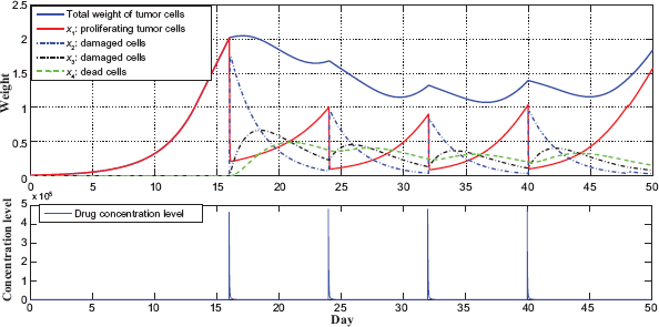
Although the experimental data sets^54,55 are not publicly available, the authors^54,55 provided the parameter values such that the tumor growth model in their papers matches their experimental data very well. Hence, we perform numerical simulation using the model given in the study^54,55 to produce synthetic data sets. Specifically, the PK data (drug plasma concentration) is generated by using the model of c(t) given by Equations (17)–(19) on page 138 of Magni et al⁵⁴ and the corresponding parameter values given in Table 2 on page 140 of Magni et al.⁵⁴ The tumor growth data during the entire treatment process is generated by firstly using the unperturbed model given by Magni et al⁵⁴ for the first 15 days, then using the perturbed model given by Magni et al⁵⁴ with the input from the PK data for 32 days (day 16 to day 47). Then the treatment is stopped from day 48 and on. In order to model the drug effect due to different drug plasma concentration, we also include the sigmoidal E_max model as given by Eq. (11) in our numerical simulation. The SIMULINK block diagrams for generating PK data and the entire treatment process are given in Figures 10 and 11, respectively. The generated synthetic data of a typical run is plotted in Figure 12 for the case of taking drug every day from day 16 to day 47.

Figure 10.

SIMULINK block diagrams for generating PK data.

Figure 11.

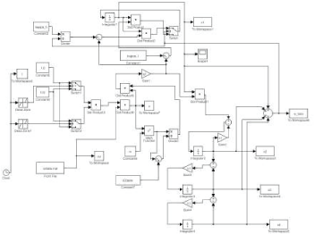
SIMULINK block diagram for generating tumor growth data during the entire treatment process.

Figure 12.

The tumor growth data from a typical run for the case of taking drug every day from day 16 to day 47.

It is observed that the tumor grows exponentially for the first 15 days, then the weight of proliferating cells x₁ dropsfrom 2 to 1.25 when drug is taken from day 16 to day 47. At the same time, the entire tumor starts growing slower and eventually reduced and stabilized. During each day, due to the PK/PD profile, x₁ reduces sharply when the initial drug concentration is high, then x₁ starts to increase because the drug concentration decreases exponentially.

Parameter Estimation

Because of the nonlinear nature of the model, we applied nonlinear least square method⁶⁹ for parameter estimation. Specifically, we use the “nlinfit“ function in MATLAB statistical toolbox. nlinfit returns the least square parameter estimates, ie, it finds the parameters that minimize the sum of the squared differences between the observed responses and their fitted values. It uses the Gauss-Newton algorithm with Levenberg-Marquardt modifications for global convergence. The detailed steps for parameter estimation is illustrated below.

Use nlinfit function to estimate the exponential growth parameter β₁ based on the measurements of the tumor size from the first 15 days and the unperturbed tumor growth model.

Now by plugging in the estimated values of β₁, $γ_{1}^{u}$ and k₁ can be estimated using nlinfit function based on the measurements of the tumor size from day 16 today 47 (when drug is taken) and the perturbed tumor growth model.

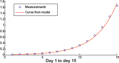
Note that since x_i(t) cannot be experimentally measured, it is not feasible to estimate the time-varying parameter $γ_{1}^{u} (t)$ directly from tumor size measurements using nonlinear least square method. Instead we consider the average effect of the drug and estimate the average value of $γ_{1}^{u} (t)$ so that nonlinear least square method is applicable. In case that the states x_i(t) and the time-varying parameter $γ_{1}^{u} (t)$ need to be estimated, Kalman filter⁷⁰ can be applied. Kalman filtering provides minimum-mean-square-error estimation of the state of a stochastic system disturbed by Gaussian white noise, since Gaussian white noise is added to the parameters for each treated subject when creating the synthetic data. This will be part of our future work.

The plot of nonlinear least square curve fitting for parameters β₁ and k₁ are given in Figures 13 and 14, respectively. It can be seen that β₁ can be accurately estimated without much error. The true value is β₁ = 0.349 and the mean of the estimates is ${\hat{β}}_{1} = 0.344$ . This is because the unperturbed tumor growth model for the first 15 days is a simple exponential curve that can be easily fitted. However, the error for estimating k₁ is large due to the complicated dynamics when drug is applied, and nonlinear curve fitting may give inaccurate estimates because only approximate expression can be obtained for the tumor growth, as also observed by Magni, Simeoni and et al.^54,55 The true value of k₁ is 0.405, while the mean of the estimates is ${\hat{k}}_{1} = 0.616$ .

Figure 13.

Curve fitting for parameter β₁.

Figure 14.

Curve fitting for parameter k₁.

Drug efficacy under different administrations

In order to obtain insights on the drug efficacy under various dosage and frequency schedules, we study the drug effect for 5 different dosing regimens with the same total drug intake, specifically, (1) once per day with the dosage given by Magni, Simeoni and et al^54,55; (2) double dosage given every two days; (3) 4 times dosage given every 4 days; (4) 8 times dosage given every 8 days; (5) 16 times dosage given every 16 days; respectively, during the 32-day (day 16 today 47) treatment process. The detailed plots for case (1) are given in Figure 12, the detailed plots for the rest cases are given in Figure 16 to 19 from Appendix B. The results are compared in Figure 15. It is observed that taking drug every 4 to 8 days seems to reduce the tumor the most, and without much oscillations. Of course, which dosing regimen to choose is depending on many other practical considerations, including toxicity. It is demonstrated that although the total drug intake during the 32-day treatment process remains the same, different dosage and frequency schedules do have significant impact on the tumor growth, which is consistent with what we obtained analytically and observed before using predefined parameters.

Figure 15.

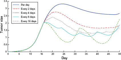
Comparison of tumor growth under different dosage and frequency schedule from day 16 today 47.

Figure 16.

The tumor growth data from a typical run for the case of taking double dosage every two days from day 16 today 47.

Figure 17.

The tumor growth data from a typical run for the case of taking 4 times dosage every 4 days from day 16 today 47.

Figure 18.

The tumor growth data from a typical run for the case of taking 8 times dosage every 8 days from day 16 today 47.

Figure 19.

The tumor growth data from a typical run for the case of taking 16 times dosage every 16 days from day 16 today 47.

Observation 4: Through this study based on synthetic data generated from experimental study,^54,55 it is clear that the parameters can be estimated by the measurements of tumor weights along the treatment process. This would enable the proposed hybrid system model to be applied to study drug effects in real-world experiments. We believe that it is feasible to refine the model with the experimentalist through an iterative process, then such model can be used to predict the drug effect and provide better recommendation for different dosing regimens.

Conclusion

A proof-of-concept study of quantitative drug effect modeling has been carried out using hybrid systems. Specifically, the PK/PD data are linked together with tumor growth dynamics in our analysis of therapeutic effects. This is a small step towards quantitative modeling of drug effect and we have kept the examples simple so that they are mathematically tractable and valuable insights can be obtained from the analytical results. For example, we have demonstrated that drug effect is closely associated with different dosing regimens and individual PK/PD characteristics, and the simulation results match the theoretical analysis. Although the examples in this paper are simple, the proposed framework for quantitative modeling of drug effect is flexible enough to be able to incorporate many practical PK/PD data as well as different models for tumor growth if desired. Of course, when more complicated PK/PD data and tumor growth models are used in the proposed framework, analytical results may not be attainable and one may have to rely on a simulation tool built on the proposed framework to obtain the drug effect for different dosing regimens and individual PK/PD characteristics.

Disclosures

Author(s) have provided signed confirmations to the publisher of their compliance with all applicable legal and ethical obligations in respect to declaration of conflicts of interest, funding, authorship and contributor ship, and compliance with ethical requirements in respect to treatment of human and animal test subjects. If this article contains identifiable human subject(s) author(s) were required to supply signed patient consent prior to publication. Author(s) have confirmed that the published article is unique and not under consideration nor published by any other publication and that they have consent to reproduce any copyrighted material. The peer reviewers declared no conflicts of interest.

Footnotes

Acknowledgements

Xiangfang Li has been supported by the National Cancer Institute (2 R25CA090301-06). The authors would like to thanks anonymous reviewers’ valuable suggestions to make this a better paper.

Proofs of Theorems

Theorem 1. Changes of the number of proliferating cells x₁ dominate the changes of all the tumor cells under drug treatment.

Proof. Firstly we express the equations of the tumor growth model under drug treatment (Eq. (3) to (7)) in matrix form

Let

It can be seen that at any given time, the solution of the matrix Eq. (41) is completely determined by the eigenvalues of matrix A. To be more specific, suppose that w_p < θ_w, then A is reduced to

It can be deduced that the diagonal terms, $β_{1} - γ_{1}^{u}$ , −k₁, −k₁, … −k₁ are the eigenvalues of matrix A. Since k₁ is always positive, the solution is completely determined by $β_{1} - γ_{1}^{u}$ . In other words, when the drug is effective, $β_{1} < γ_{1}^{u}$ , then all the eigenvalues of A are negative, and the number of cells in all stages will decrease. On the contrary, when $β_{1} > γ_{1}^{u}$ , the first eigenvalue of A is positive, the solution will be exponentially increasing. Hence, the number of cells in all stages depends on the dynamics of number of proliferating cells x₁. A similar conclusion can be drawn when w_p > θ_w. Thus the theorem follows.

Theorem 2. The change of proliferating tumor size in one treatment, defined as x₁((k + 1)τ_i) — x₁(kτ_i), is a strictly convex function of time interval t_i.

Proof. We define the reduction of proliferating tumor size in one treatment as

To show that Δx₁ is a strictly convex function of time interval τ_i, we need to prove that the second derivative of Δx₁ with respect to τ_i is positive for any τ_i. We show the case where the trajectory starts from domain D₅; similar techniques can be used to show it for the other case where the trajectory starts from domain D₃. When the drug dosage is high enough, ie, $ζ_{i} > \bar{θ}$ , we have

Now the first derivative of Δx₁ with respect to τ_i is given by

where $a_{1} = q_{1}^{u} / λ_{d}$ and $a_{3} = \bar{θ} - \underline{θ}$ . Then the second derivative of Δx₁ with respect to τ_i can be derived as

Since both x₁(kτ_i) and e^Ψ are positive, we only need to show that

which is equivalent to

It is straightforward to verify that the above inequality (49) is always true since a₁ > 0, a₃ > 0, β₁ > 0. Then the theorem follows.

Detailed plots for Section “Parameter Estimation”

In order to demonstrate that drug effect is depending on the dosing regimens given the same total drug intake, detailed drug effect plot is showed in this appendix. While Figure 12 provides the case for taking drug every day from day 16 to day 47, the following figures are the detailed plots for: double dosage given every two days (Fig. 16); 4 times dosage given every 4 days (Fig. 17); 8 times dosage given every 8 days (Fig. 18); 16 times dosage given every 16 days (Fig. 19); respectively, during the 32-day (day 16 to day 47) treatment process.

References

Hait

W.N.

Anticancer drug development: the grand challenges.

Nature Reviews Drug Discovery. 2010; 9: 253–4.

Kola

, Landis

Can the pharmaceutical industry reduce attrition rates?

Nat Rev Drug Discov. 2004; 3(8): 711–5.

Giersiefen

, Hilgenfeld

, Gukkuscg

Modern methods of drug discovery: A introduction.

In Modern Methods of Drug Discovery. Edited by Hillisch

, Hilgenfeld

, Germany: Birkhuser Verlag; 2002.

Kamb

What's wrong with our cancer models?

Nat Rev Drug Discov. 2005; 4(2): 161–5.

Rajman

PK/PD modeling and simulations: utility in drug development.

Drug Discov Today. 2008; 13(7-8): 341–6.

Quaranta

, Weaver

, Cummings

, Anderson

Mathematical modeling of cancer: The future of prognosis and treatment.

Clinica Chimica Acta. 2005; 357: 173–9.

Searls

D.B.

Data Integration: Challenges for drug discovery.

Nature Reviews Drug Discovery. 2005; 4: 45–58.

Alexander

, Anderson

, Quaranta

Integrative mathematical oncology.

Nature Reviews Cancer. 2008; 8: 227–34.

Hood

, Perlmutter

R.M.

The impact of systems approaches on biological problems in drug discovery.

Nature Biotechnology. 2004; 22(10): 1215–7.

10.

Kumar

, Hendriks

, Janes

, Graaf

, Lauffenburger

Applying computational modeling to drug discovery and development.

Drug Discovery Today. 2006; 11: 806–11.

11.

Butcher

, Berg

, Kunkel

System biology in drug discovery.

Nature Biotechnology. 2004; 22: 1253–9.

12.

Jones

Steps on the road to personalized medicine.

Nature Reviews Drug Discovery. 2007; 6: 770–1.

13.

Ting

Introducton and new drug development process.

In Dose Finding in Drug Development. Edited by Ting

, New York, NY: Springer 2006.

14.

Gieschke

, Steimer

J.L.

Pharmacometrics: modeling and simulation tools to improve decision making in clinical drug development.

European Journal of Drug Metabolism and Pharmaco Kinetics. 2000; 25: 49–58.

15.

Undevia

, and M Ratain

G.G.A.

Pharmacokinetic variability of anticancer agents.

Nature Reviews Cancer. 2005; 5: 447–58.

16.

Saif

M.W.

, Choma

, Salamone

, Chu

Pharmaco kinetically guided dose adjustment of 5-fluorouracil: a rational approach to improving therapeutic outcomes.

J Natl Cancer Inst. 2009; 101(22): 1543–52.

17.

Baker

, Verweij

, Rowinsky

. Role of body surface area in dosing of investigational anticancer agents in adults, 1991–2001. J Natl Cancer Inst. 2002; 94(24): 1822–3.

18.

Sangkuhl

, Berlin

D.S.

, Altman

R.B.

, Klein

T.E.

Pharm GKB: Understanding the effects of individual genetic variants.

Drug Metabolism Reviews. 2008; 40(4): 539–51.

19.

Group BDW.

Biomarkers and surrogate endpoints: proposed definitions and conceptual framework.

Clin Pharmacol Ther. 2001; 69: 89–95.

20.

Shah

, Kasap

, Weier

. Transient potent BCR-ABL inhibition is sufficient to commit chronic myeloid leukemia cells irreversibly to apoptosis. Cancer Cell. 2008; 14(6): 485–93.

21.

Amin

, Sergina

, Ahuja

. Resiliency and vulnerability in the HER2-HER3 Tumorigenic Driver. Science Transitional Medicine. 2010; 2(16): 1–9.

22.

Rajasethupathy

, Vayttaden

, Bhalla

Systems modeling: a pathway to drug discovery.

Current Opinion in Chemical Biology. 2005; 9: 400–6.

23.

Butcher

Can cell systems biology rescue drug discovery?

Nature Reviews Drug Discovery. 2005; 4: 461–67.

24.

Deisboeck

T.S.

, Zhang

, Martin

Advancing cancer systems biology: Introducing the Center for the Development of a Virtual Tumor, CViT.

Cancer Informatics. 2007; 5: 1–8.

25.

Materi

, Wishart

D.S.

Computational systems biology in cancer: Modeling methods and applications.

Gene Regulation and Systems Biology. 2007; 1: 91–110.

26.

Dougherty

E.R.

Translational Science. Epistemology and the investigative process.

Current Genomics. 2009; 10(2): 102–9.

27.

Hanahan

, Weinberg

R.A.

The hallmarks of cancer.

Cell. 2000; 100: 57–70.

28.

Ideker

, Lauffenburger

Building with a scaffold: emerging strategies for high-to low-level cellular modeling.

Trends in Biotechnology. 2003; 21(6): 255–62.

29.

Coveney

P.V.

, Fowle

P.W.

Modelling biological complexity: a physical scientists perspective.

Journal of The Royal Society Interface. 2005; 2: 267–80.

30.

Sorger

P.K.

A reductionist's systems biology: Opinion.

Current Opinion in Cell Biology. 2005; 17: 9–11.

31.

Szallasi

, Stelling

, Periwal

System Modeling in Cell Biology: From Concepts to Nuts and Bolts. Cambridge, MA: MIT Press 2006.

32.

Schaft

, Schumacher

An Introduction to Hybrid Dynamical Systems.

Lecture Notes in Control and Information Sciences, 251, London: Springer 2000.

33.

Lincoln

, Tiwari

Symbolic Systems Biology: Hybrid Modeling and Analysis of Biological Networks. In Hybrid Systems: Computation and Control HSCC, Volume 2993. Edited by Alur

, Pappas

, Springer 2004: 660–72.

34.

Glass

, Kauffman

The logical analysis of continuous non-linear biochemical control networks.

Journal of Theoretical Biology. 1973; 39: 103–29.

35.

de Jong

Modeling and simulation of genetic regulatory systems: A literature review.

Journal of Computational Biology. 2002; 9: 67–103.

36.

Santillan

, Mackey

Quantitative approaches to the study of bistability in the lac operon of escherichia coli.

J. Roy. Soc., Interface the Royal Society. 2008; 5.

37.

Muller-Hill

The lac operon: A short history of agenetic paradigm. Walterde Gruyter. 1996.

38.

Halasz

, Kumar

, Imielinski

. Analysis of lactose metabolism in E. coli using reachability analysis of hybrid systems. IET Systems Biology. 2007; 1: 120–48.

39.

Ghosh

, Tiwari

, Tomlin

Automated symtolic reachability analysis; with application to delta-notch signaling automata.

Hybrid Systems: Compuation and Control. 2003; 233–48.

40.

Ghosh

, Tomlin

Symbolic reachable set computation of piecewise affine hybrid automata and its application to biological modelling: Delta-Notch protein signalling.

IET Systems Biology. 2004; 1: 170–83.

41.

Drulhe

, Ferrari-Trecate

, de Jone

, Viari

Reconstruction of switching thresholds in piecewise-affine models of genetic regulatory networks.

Hybrid Systems: Compuation and Control. 2006; 184–99.

42.

Batt

, Ropers

, de Jone

, Geiselmann

, Page

, Schneider

Qualitative analysis and verification of hybrid models of genetic regulatory networks: Nutritional stress response in Escherichia coli.

Hybrid Systems: Compuation and Control. 2006; 134–50.

43.

, Qian

, Bittner

, Dougherty

Characterization of drug efficacy regions based on dosage and frequency schedules.

IEEE Transaction on Biomedical Engineering. 2010; 58(3): 488–98.

44.

Swanson

K.R.

, Bridge

, Murray

J.D.

, Alvord

E.C.

Virtual and real brain tumors: using mathematical modeling to quantify glioma growth and invasion.

Journal of the Neurological Sciences. 2003; 216: 1–10.

45.

Collins

V.P.

, Loeffler

R.K.

, Tivey

Observations on growth rates of human tumors.

Am J Roentgenol Radium Ther Nucl Med. 1956; 76(5): 988–1000.

46.

Kusama

, Spratt

J.S.

, Donegan

W.L.

, Watson

F.R.

, Cunningham

The gross rates of growth of human mammary carcinoma.

Cancer. 1972; 30(2): 594–9.

47.

Goldie

J.H.

, Coldman

A.J.

Drug Resistance in Cancer: Mechanisms and Models. Cambridge University Press. 1998.

48.

Bajzer

, Marusic

, Vuk-Pavlovi

Conceptual frameworks for mathematical modeling of tumor growth dynamics.

Mathematical and Computer Modelling. 1996; 23(6): 3146.

49.

Norton

A Gompertzian model of human breast cancer growth.

Cancer Res. 1988; 48: 7067–71.

50.

Spraft

J.A.

, von Fournier

, Spraff

J.S.

, Weber

E.E.

Decelerating Growth and human breast cancer.

Cancer. 1993; 71: 2013–19.

51.

Marusic

, Bajzer

, Freyer

, Vuk-Pavlovic

Analysis of growth of multicellular tumour spheroids by mathematical models.

Cell Proliferation. 1994; 27: 73–94.

52.

Gasparini

, Biganzoli

, Bonoldi

, Morabito

, Fanelli

, Boracchi

Angiogenesis sustains tumor dormancy in patients with breast cancer treated with adjuvant chemotherapy.

Breast Cancer Res Treat. 2001; 65: 71–5.

53.

Steimer

, Dahl

, Alwis

D.D.

. Modelling the genesis and treatment of cancer: the potential role of physiologically based pharmacodynamics. European Journal of Cancer. 2010; 46: 21–32.

54.

Magni

, Simeoni

, Poggesi

, Rocchetti

, Nicolao

G.D.

A mathematical model to study the effects of drugs administration on tumor growth dynamics.

Mathematical Bio Sciences. 2006; 200: 127–51.

55.

Simeoni

, Magni

, Cammia

. Predictive pharmacokinetic-pharmacodynamic modeling of tumor growth kinetics in xenograft models after administration of anticancer agents. Cancer Research. 2004; 64: 1094–101.

56.

Rocchetti

, Simeoni

, Pesenti

, Nicolao

G.D.

, Poggesi

Predicting the active doses in humans from animal studies: A novel approach in oncology.

European Journal of Cancer. 2007; 43: 1862–8.

57.

Barbolosi

, Iliadis

Optimizing drug regimens in cancer chemotherapy: a simulation study using a PK-PD model.

Computers in Biology and Medicine. 2001; 31(3): 157–72.

58.

Usher

J.R.

Some mathematical models for cancer chemotherapy.

Computers & Mathematics with Applications. 1994; 28(9): 73–80.

59.

Derendorf

, Meibohm

Modeling of pharmacokinetic/pharmacodynamic (PK/PD) relationships: concepts and perspectives.

Pharmaceutical Research. 1999; 16(2): 176–85.

60.

Prez-Urizar

, Granados-Soto

, Flores-Murrieta

F.J.

, Castaeda-Hernndez

Pharmacokinetic-pharmacodynamic modeling: Why?

Archives of Medical Research. 2000; 31(6): 539–45.

61.

Chien

J.Y.

, Friedrich

, Heathman

M.A.

, de Alwis

D.P.

, Sinha

Pharmacokinetics/pharmacodynamics and the stages of drug development: role of modeling and simulation.

The AAPS Journal. 2005; 7(3): 544–59.

62.

Meibohm

, Derendorf

Pharmacokinetic/pharmacodynamic studies in drug product development.

Journal of Pharmaceutical Sciences. 2002; 91: 18–31.

63.

Kuh

, Jang

, Wientjes

, AU

Computational Model of Intracellular Pharmacokinetics of Paclitaxel.

Journal of Pharmacology and Experimental Therapeutics. 2000; 293(3): 761–70.

64.

Hill

A.V.

The possible effects of the aggregation of the molecules of haemoglobin on its dissociation curves.

J Physiol. 1910; 40: iv–vii.

65.

Holford

N.H.

, Sheiner

L.B.

Understanding the dose-effect relationship: clinical application of pharmacokinetic-pharmacodynamic models.

Clin Pharmacokinet. 1981; 6(6): 429–53.

66.

Waud

D.R.

, Parker

R.B.

Pharmacological estimation of drug-receptor dissociation constants. Statistical evaluation. II. competitive antagonists.

J Pharmacol Exp Ther. 1971; 177: 13–24.

67.

Levasseur

L.M.

, Slocum

H.K.

, Rustum

Y.M.

, Greco

W.R.

Modeling of the time-dependency of in vitro drug cytotoxicity and resistance.

Cancer Research. 1998; 15(58): 5749–61.

68.

Bertsekas

D.P.

, Nedic

, Ozdaglar

A.E.

Convex Analysis and Optimization. Athena Scientific. 2003.

69.

Bates

, Watts

D.G.

Nonlinear Regression Analysis and Its Applications. New York: Wiley 1988.

70.

Grewal

, Andrews

Kalman Filtering: Theory and Practice. Englewood Cliffs, NJ: Prentice Hall 1993.