Sage Journals: Discover world-class research

Abstract

Keywords

recurrent copy number variation cancer interval graph maximal clique

Introduction

Structural variation includes rearrangements (inversions and translocations) and copy number variations (CNVs), consisting of duplications, deletions, insertions, and multi-allelic variations ranging from one kilobase (kb) to several megabases of DNA, leading to possible dosage imbalances. In other words, genes that were originally understood to be present in two copies have now been revealed to sometimes exist in one, three, more than three copies, or even missing altogether. We define a CNV as a DNA segment that is 1 kb or larger and exists at variable copy numbers when referred to a reference genome.¹

So far, among the numerous insights gained from the completion of the Human Genome Project, single nucleotide polymorphisms (SNPs) have been recognized as a major source of genetic variation, which led to the speculation that the majority of phenotypic variations in humans are due to SNPs.¹ Consequently, immense amount of research has focused on developing genotyping assays and methodologies for SNP analysis, making it the most frequently assayed type of intraspecific genetic variation and the most centered gene-mapping studies with regard to the relationship between SNPs and human diseases. However, growing number of studies have confirmed that more nucleotide bases are affected by CNVs as opposed to SNPs between any two individuals,² and along with the advances in high-throughput technologies to detect the magnitude and location of genomic alterations within a single human genome, it is clear that large fragments of our genome have been deleted or duplicated. These structural variations can change the genes copy number that encompass the affected regions and alter gene regulation. In particular, one group of scientist conducted a pilot study in mapping the CNVs in the complete human genome,² which demonstrated the remarkable extent of large structural variation in the human genome, both within closely related people and between the global populations due to sizeable duplications and deletions of genomic segments. Likewise, similar studies have shown that despite the existence of powerful repair mechanisms in the human genome, CNV occurrence frequency is 100–10,000 times higher than point mutations.³

Studies have shown that some types of genes are more prone to be copy number variables than others, such as the genes involved in immunological and neurological development, possibly due to the rapid human evolution in these two functions.^4,5 On the other hand, genes that play a role in early development and mitosis, which are fundamental to life, are likely to be spared.⁵ CNVs have been reported to play a role in cancer susceptibility, formation, and progression.^6–8 These CNVs may be germline variants or somatic mutations. A few association studies have already elucidated the significance of CNVs as disease-susceptibility variants.^9–12 In one study, CNV detected in 1,400 regions have overlaps with 14.5% of human disease-causal genes.⁹ Recent studies concluded that CNV is frequently found in susceptible individuals who were predisposed to diseases such as color blindness in Mendelian disease, as well as autism, Parkinson's, HIV, cancer, and lupus in complex traits diseases.^10–16

This intriguingly frequent and dynamic type of genomic variation has challenged the concept of analyzing the genome through the breakdown of a single diploid human reference genome and has also triggered more research on the techniques of detecting CNVs. Array comparative genome hybridization (aCGH) is a popular experimental technique for detecting copy number variants in genomes.^17–19 aCGH requires the hybridization of fluorescently tagged differential DNA fragments from both a test genome and a reference genome to a set of probes originated from the reference genome sequence. The proportion of the test versus reference fluorescence intensity at each probe will identify the positions in the test genome that have fewer, more, or similar copy as the reference genome, which can generate a copy number profile of the test genome.^17–19 These CNV profiles are generally compared across individuals in a group of interest to identify common CNVs that are shared among a portion of the group.

Another method that is popular for CNV detection and analysis is by using high-throughput array technologies for SNP genotyping from commercial companies such as Affymetrix and Illumina, due to their ability to perform a dual role for both SNP-based and CNV-based association studies. One widely used array is the Affymetrix genome-wide human SNP array 6.0 (Affy6), which is an array platform that aims to perform both high-density SNP genotyping and high-resolution CNV discovery simultaneously. Aside from the 906,600 SNP probe sets, the Affy6 array also contains 946,000 copy number probe sets that can be used to assess chromosomal copy number changes in regions of the genome that are not well covered by SNPs.

A number of CNV calling methods for individual patients have been implemented, which either follows the circular binary segmentation (CBS) method or the hidden Markov model (HMM) method. CBS is a segmentation-based method that scans for change points in an ordered sequence of values to delineate segments with different distributions of values (measured by having different means). In other words, it will recursively divide up the genome until segments that have probe distribution different than neighbors have been identified.²⁰ For the HMM method, the aim is to uncover the hidden copy number states (0, 1, 2, 3 copies, etc) by searching the data point by point to determine the most probable copy number states based on observation and transitions between states correspond to changes in copy number.^21,22

These methods share a common feature in which the CNV regions are segmented by individual-specific breakpoints, and detection is carried out sample by sample. However, it is much more likely for shared/common CNV regions (ie, recurrent CNV) to occur at the same genomic positions across different individuals in a homogeneous group of people. As a result, recurrent CNV regions are more likely to harbor disease-causal genes, as it is more probable to encompass “driver” alterations (functionally significant for disease initiation or progression), while individual-sample CNVs are subject specific and would be more likely to contain “passenger” alterations (random somatic events irrelevant to pathological events) than disease-relevant alterations.²³ Several methodologies have been proposed for recurrent CNV detection.^24–29 These methods mainly differ in the type of input data and the algorithm models being implemented. For the input, most of the recurrent CNV detection methods fall under two categories: continuous (log 2 ratio)^25,27,28 and discrete (gains/losses).^24,26,29 For the algorithms, they can be categorized into three main models: permutation,^24,27 probabilistic null model,^25,28–30 or none.²⁶

In this study, we aim to develop a graph-based algorithm to identify recurrent CNV regions. The algorithm will be applied to analyze the breast cancer data retrieved from Molecular Taxonomy of Breast Cancer International Consortium (METABRIC).³¹

Materials and Methods

Data Source

We retrieved the individual patient-level CNV data from METABRIC,³¹ which consists of whole-gene expression profiles, SNPs, and individual patient-level DNA CNV data. All samples were derived from ~2,000 clinically annotated primary fresh-frozen breast cancer specimens from tumor banks in the UK and Canada, which were divided into two subsets by METABRIC: Discovery (997 samples) and Validation (995 samples).

Experimental Assay and Genotype Calling

DNA was extracted from each tumor specimen and subject to copy number analysis on the Affymetrix Human SNP 6.0 platform. Data from Affymetrix SNP 6.0 arrays were preprocessed and genotyped using the SNP-RMA (Robust Multi-Array Average) algorithm, available in the crlmm Bioconductor R package. This quantifies raw intensity values into proportional amount of DNA in the target sample associated with each of the alleles, A and B, for each SNP. Feature intensities were corrected for fragment length and sequence effects, followed by quantile normalization to a predefined reference distribution. Intensities were then summarized by median polish, with a single value for each allele. A mixture model was then used to adjust for remaining fragment length and intensity-dependent biases on the log ratio of the summarized intensities. Samples with a signal-to-noise ratio <5 were flagged in downstream analyses.

Individual CNV Calling

Affymetrix SNP 6.0 arrays were preprocessed for copy number segmentation using aroma. affymetrix. Both tumor and normal samples were independently normalized using the single-array method referred to as copy number estimation using robust multichip analysis³² (CRMAv2), along with a publicly available SNP 6.0 data set consisting of 270 HapMap individuals. For each sample, allelic cross-talk calibration, probe sequence effects normalization, probe-level summarization, and polymerase chain reaction fragment length normalization were performed in order to obtain log 2 intensity values for total copy number estimation. Afterward, probes were sorted by their genomic position, replicate probes were summarized by their median value, and missing values (generated by negative intensities in the normalization) were imputed using the loess procedure included in the snapCGH Bioconductor R package.

Two pooled references were generated, one using the median intensities across the HapMap individuals and another for the normals and tumors, using the median intensity values from a set of 473 normals. Next, log 2 ratios were generated for the HapMap samples by subtracting the pooled value from the log 2 intensities. Similarly, log 2 ratios were obtained for the 473 normals using the corresponding pool. For the 997 tumor samples, two data sets were produced: one using the normal pool as the reference for all the tumors and another using the matched normal for each tumor when available, and the normal pool for the remainder. A similar approach was taken for the validation set.

The HapMap and normal data sets were used to estimate the frequency of germline CNVs in the cohort, while the tumor samples were used for estimating somatic CNVs. After computing the log 2 ratios for each probe, samples were segmented using the CBS algorithm implemented in the DNAcopy R Bioconductor package and individual patient-level CNVs were called. For the tumor samples, any segmented mean that fell within a region included in the HapMap+Normals CNV list was labeled as an inherited CNV. In order to remove all possible germline CNVs, the frequencies of somatic CNVs in the tumor samples were obtained after removing the germline CNVs from the normalized pool reference. For the Discovery data set, a total of 13,391 individual patient-level CNV gains and 20,540 individual patient-level CNV losses were detected. For the Validation data set, a total of 13,963 individual patient-level CNV gains and 20,308 individual patient-level CNV losses were detected.

Identification of Recurrent CNVs

Representing CNVs as an Interval Graph.

We denote a CNV segment as R_j = (l_j, r_j), where j is the jth CNV and l_j, r_j are its left and right chromosome positions. For a CNV set, we have R = {R₁, R₂, …, R_n}. When r is infinite, we call R is a right-censored univariate data set. An intersection graph can easily be constructed from R as follows: each member in R corresponds to a vertex which we denote by its index. Hence, R_j corresponds to vertex j. We denote the set of vertices as V. Two vertices j and k are linked by an edge if the corresponding members R_j and R_k in R are intersected. We denote the edge as jk and the set of edges as E. When the R is a linearly ordered set, the intersection graph is called an interval graph, and all interval graphs are triangulated.

Figure 1A shows the examples of six individual patient-level CNV segments (A, B, C, D, E, F) on the same chromosome. Each of the six CNVs contains chromosomal-specific start (left) and end (right) positions. To identify the common regions of individual patient-level CNVs on the same chromosome, the intersection among the individual patient-level CNVs can be represented as an interval graph, treating each called individual patient-level CNV as a vertex of the graph and connecting two vertices only if the corresponding intervals have an intersecting region. Thus, the constructed interval graph G(V,E) is composed of a set of vertices V, where each vertex (v∈V) corresponds to a specific interval of the individual patient-level CNV and each edge ({u,v}∈E) connects two intersecting intervals u and v. In Figure 1B, an example of the interval graph is shown where A through E are the intervals (nodes of the graph or individual patient-level CNVs) and an edge connects two nodes (individual patient-level CNVs) if the intervals overlap.

Figure 1.

Representing CNVs as an interval graph. (A) A, B, C, D, E, F are individual patient-level CNVs on a specific chromosome. Each of the CNVs has chromosome start and end positions. (B) this is an interval graph where A, B, C, D, E, F are the individual patient-level CNVs in (A). The edge between each of the two vertices in the graph represents that the two individual patient-level CNVs share a piece of common regions on the chromosome.

Finding Maximal Cliques from an Interval Graph.

A clique is a set of vertices in which any two vertices are connected by an edge in the interval graph. A maximal clique is a clique that cannot be a subclique of a larger clique. In the context of a CNV set R, a clique can be viewed as a set of CNV segments whose regions intersect. For example, Figure 1B shows that {A, B, C, D} is a maximal clique, as it cannot be extended by adding any other vertices. However, {A, C, D} is not a maximal clique but a clique, as it can be extended by adding vertex B to it.

To find maximal cliques in an interval graph constructed from individual patient-level CNVs, we applied the algorithm of Gentleman and Vandal.³³ The main idea of the algorithm is to sort the vertices based on their chromosomal end positions. The ordering is important because it allows the algorithm to discard vertices in each iteration without losing the triangulation property. The input of the algorithm is the individual patient-level CNVs on a specific chromosome, which include two parameters for each CNV segment: start and end positions (base pair). It should be noted that we need to analyze CNV gains and losses separately. The algorithm adapted for processing individual patient-level CNV data is summarized as follows:

Algorithm

Finding the maximal cliques M

Sort all the vertices in terms of their chromosomal end positions

Initialize M = {} and k = 0, where k is the kt^h maximal clique

For each vertex v, initialize S(v) = 0, where S(v) is the number of neighbors of v

For each vertex v, check

if adjacent neighbor of v, adj(v) is empty, $k = k + 1, M_{k} = {v}, M \cup M_{k}$

else

X_v = adj(v), where X_v is the set of neighbos of vertex v

S(u) = max{S(u),|X_v|-1}, where u is the next vertex to be eliminated

if S(v)(|X_v|

$k = k + 1, M_{k} = {v}, \cup X_{v}, M \cup M_{k}$

else eliminate v

return M

The output of the algorithm will be a list of maximal cliques. We implemented the algorithm using R package Icens,³³ which implemented the algorithm to find maximal cliques of a triangulated graph based on the fact that all interval graphs are triangulated.³⁴ The method is efficient and the time complexity of the maximal clique detection algorithm is O(n+e), where e is the total number of edges in the corresponding graph.

Analyzing Recurrent CNVs from the Maximal Cliques.

Each of the identified maximal cliques is a recurrent CNV, which is common in multiple patients. The shared region of the recurrent CNV across multiple patients is the minimal common region (MCR) of the CNV, which has the potential to harbor cancer-causing genes. In practice, the size of the maximal cliques should be at least 2 and the size of the MCRs should be at least 1 kb.

Unlike the algorithm of Gentleman and Vandal to identify maximal cliques, Wu et al.³⁵ also proposed an algorithm to identify maximal cliques for detecting recurrent CNVs. However, this algorithm is based on a scoring scheme where blocks of consecutive maximal cliques were scored, defining a pivot within the block and calculating the number of left and right end position pairs that crosses that pivot.

Results

Figure 2 shows our analysis flowchart using the maximal clique-based recurrent CNV detection. The individual patient-level CNV data in Discovery data set containing 997 patient samples was separated into two CNV types: gain and loss. Filtering criteria include retaining CNV data that were generated by ≥10 probes and having a CNV size of at least 5 kb. Among the total 997 patients, there are 13,391 individual patient-level CNV gain regions and 20,540 individual patient-level CNV loss regions. The recurrent CNV calling algorithm was run separately for the CNV gains and CNV losses, and analysis was done chromosome by chromosome. Further filtering at the recurrent CNV level includes retaining those that have a minimal region of at least 1 kb, and the number of patients per recurrent CNV region to be at least 5. In total, there are 351 recurrent CNV gain regions (99/351 gain regions encompassing protein-encoding genes) and 475 recurrent CNV loss regions (111/475 loss regions encompassing protein-encoding genes).

Figure 2.

Flowchart analysis for implicating proposed algorithm.

Validation testing was then performed using the Validation data set, which contains 995 patient samples. All filtering criteria and algorithm implementations followed the same procedure as the Discovery data set analysis. For recurrent CNV gain regions, a total of 252 regions have been validated (found in both the Discovery and Validation data sets), of which 67/252 regions have encompassed 57 unique protein-encoding genes (Supplementary Tables 1 and 2). For recurrent CNV loss regions, a total of 350 regions have been validated, of which 77/350 regions have encompassed 70 unique protein-encoding genes (Supplementary Tables 3 and 4). In total, 144 validated recurrent CNV regions with protein-encoding genes have been identified, along with 458 validated recurrent CNV regions that did not encompass any protein-encoding genes. There is no significant difference of the validated number of CNV gain and loss regions in both Discovery and Validation data sets (P-value = 0.58, Fisher's exact test). Figure 3A and B shows the number of patients identified in validated recurrent CNV gain regions with the protein-encoding genes (A) and without any genes (B), respectively. It appears that most of the recurrent CNV gain regions have similar number of patients in Discovery and Validation sets. We also observed the same trend in the validated recurrent CNV loss regions with the protein-encoding genes (C) and without any genes (D), respectively. Since the number of patients in Discovery and Validation sets are similar (997 vs. 995), the Y-axis in Figure 3A–D is also called as the proportion of the patients.

Figure 3.

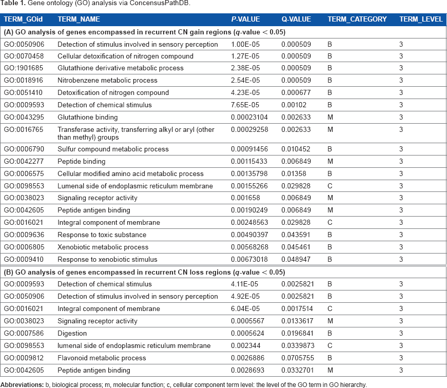
Comparison of the number patients in each recurrent CNV in Discovery set and Validation set. The number of patients in validated recurrent gain CNV regions with genes (A) and without genes (B) and in validated recurrent loss CNV regions with genes (C) and without genes (D).

Table 1.

Gene ontology (Go) analysis via ConcensusPathDB.

TERM_GOid	TERM_NAME	P-VALUE	Q-VALUE	TERM_CATEGORY	TERM_LEVEL
(A) Go analysis of genes encompassed in recurrent CN gain regions (q-value < 0.05)
GO:0050906	Detection of stimulus involved in sensory perception	1.00e-05	0.000509	B	3
GO:0070458	Cellular detoxification of nitrogen compound	1.27e-05	0.000509	B	3
GO:1901685	Glutathione derivative metabolic process	2.38e-05	0.000509	B	3
GO:0018916	nitrobenzene metabolic process	2.54e-05	0.000509	B	3
GO:0051410	Detoxification of nitrogen compound	4.23e-05	0.000677	B	3
GO:0009593	Detection of chemical stimulus	7. 6 5 e-0 5	0.00102	B	3
GO:0043295	Glutathione binding	0.00023104	0.002633	M	3
GO:0016765	Transferase activity, transferring alkyl or aryl (other than methyl) groups	0.00029258	0.002633	M	3
GO:0006790	Sulfur compound metabolic process	0.00091456	0.010452	B	3
GO:0042277	Peptide binding	0.00115433	0.006849	M	3
GO:0006575	Cellular modified amino acid metabolic process	0.00135798	0.01358	B	3
GO:0098553	Lumenal side of endoplasmic reticulum membrane	0.00155266	0.029828	C	3
GO:0038023	signaling receptor activity	0.001658	0.006849	M	3
GO:0042605	Peptide antigen binding	0.00190249	0.006849	M	3
GO:0016021	Integral component of membrane	0.00248563	0.029828	C	3
GO:0009636	Response to toxic substance	0.00490397	0.043591	B	3
GO:0006805	Xenobiotic metabolic process	0.00568268	0.045461	B	3
GO:0009410	Response to xenobiotic stimulus	0.00673018	0.048947	B	3
(B) GO analysis of genes encompassed in recurrent CN loss regions (q-value < 0.05)
GO:0009593	Detection of chemical stimulus	4.11E-05	0.0025821	B	3
GO:0050906	Detection of stimulus involved in sensory perception	4.92E-05	0.0025821	B	3
GO:0016021	Integral component of membrane	6.04E-05	0.0017514	C	3
GO:0038023	Signaling receptor activity	0.0005567	0.0133617	M	3
GO:0007586	Digestion	0.0005624	0.0196841	B	3
GO:0098553	Lumenal side of endoplasmic reticulum membrane	0.002344	0.0339873	C	3
GO:0009812	Flavonoid metabolic process	0.0026886	0.0705755	B	3
GO:0042605	Peptide antigen binding	0.0028693	0.0332701	M	3

Abbreviations: b, biological process; m, molecular function; c, cellular component term level: the level of the GO term in GO hierarchy.

Gene set pathway overrepresentation analysis was performed separately for the 67 validated recurrent CNV gain regions (Supplementary Table 1) and 77 validated recurrent CNV loss regions (Supplementary Table 3) via Consensus-PathDB with default settings (http://consensuspathdb.org/). Enrichment map analysis was then performed using the software Cytoscape (http://www.cytoscape.org/). For the recurrent CNV gain regions, an enrichment in the glutathione metabolism pathway involving cytochrome 450 is detected (Fig. 4A), with genes GSTM2 and GSTT1 playing a major role in this pathway. For the recurrent CNV loss regions, an enrichment in the metabolism pathway involving starch and sucrose digestion is detected (Fig. 4B), with genes AMY1A and MGAM playing a major role in this pathway.

Figure 4.

Pathway enrichment map generated by Cytoscape. (A) Pathway enrichment map for the 67 validated recurrent CNV gain regions. (B) Pathway enrichment map for the 77 validated recurrent CNV loss regions. Each solid circle represents one pathway. Edge thickness represents overlap between two pathways. Color represents P-value – the redder the color, the lower the P-value. Node size represents the size of the pathway. Pathways with similar biological meanings were clustered, and a name was assigned to each cluster in the map using text-mining application “WordCloud” within Cytoscape. The generated name acts as a general representative of the cluster.

Gene ontology analysis was performed to determine the functions of the genes encompassed within the recurrent CNV gain (Table 1A) and loss regions (Table 1B). Overall, majority of the genes in both the recurrent CNV gain and loss regions play a role in sensory perception, especially in G-protein coupled receptor (GPCRs) events and chemical stimulus detection. GPCRs constitute a large family of proteins that sense extracellular stimuli and activate intracellular signal transduction and have been shown to be crucial players in tumor growth and metastasis.³⁶ This finding came from the observation that in order for tumor cells to survive and proliferate, they often seize control of the normal physiological functions of GPCRs, including evasion of the immune system, increase in their blood supply, invasion of surrounding tissues, and metastasis to other organs.³⁶ Chemical carcinogenesis is another major pathway found involving the role of chemical stimulus detection. GSTT1 and GSTM2, members of the glutathione S-transferase (GST) superfamily, have been widely studied in cancer risk with regard to the homozygous deletion of the gene (GSTM1 null), leading to a lack of corresponding enzymatic activity. Since tumorigenesis requires suppression of the apoptotic and anti-proliferative effects of p38 MAPK pathway, it has been proposed that tumor cells can uncouple ROS production from the p38 MAPK activation in order to overcome the tumor-suppressive roles of p38 MAPK, and the increased expression of GSTM proteins in these tumor cells may serve this function.³⁷ By acting as ROS sensors suppressing the p38 MAPK pathway, the GStm proteins were proposed to be good candidate drug targets for cancer therapies.³⁷

Conclusion

In this study, we first propose how to build an interval graph based on individual patient-level CNVs. A maximal clique-based graph algorithm is then applied to call recurrent CNVs in breast cancer patients. The algorithm has an optimal solution, which means all maximal cliques can be identified. Additionally, it guarantees that the identified CNV regions are the most frequent and that the minimal regions have been delineated. Our algorithm is based on the sample-specific CNVs called from other published CNV calling algorithms. Therefore, the potential uncertainties or errors in our identified recurrent CNVs will depend on the sample-specific CNVs identified by other algorithms. From application to the METABRIC breast cancer data set, we have identified 252 validated recurrent CN gain regions and 350 validated recurrent CN loss regions and have located the corresponding candidate genes that were encompassed in these regions. It should be noted that the algorithm has also been successfully used to identify and validate recurrent CNV-based genomic signatures in circulating tumor cells from breast cancer,^38,39 but the algorithm details have not been described in those applications.

It is becoming progressively clear that genetic studies of complex diseases must heed to the involvement of recurrent CNVs. Therefore, investigation into recurrent CNVs could provide significant contributions to the understanding of the basis of genetic variations in biological functions and disease predisposition. At present, CNV studies with regard to cancer are still in its infancy, but it is an area that is growing rapidly due to denser microarrays and next-generation sequencing technologies. As we lean toward personalized structural genomic analysis and diagnostics, the conventional genomic definition of what is “normal” versus “diseased” will start to blur. There is much to take in from previous studies on genomic disorders and by incorporating the knowledge of the vast amount of CNVs present in our genome. It can give new insights into the role of CNVs in cancer predisposition and development and contribute to a more accurate and complete human genome sequence reference.

Author Contributions

Conceived and designed the experiments: PH. Prepared data: QK. Analyzed the data: CC. Wrote the first draft of the manuscript: CC, RA, PH. Contributed to the writing of the manuscript: CC, RA, PH, QK. Agreed with manuscript results and conclusions: All authors. Made critical revisions and approved final version: CC, RA, PH. All authors reviewed and approved the final manuscript.

Footnotes

Acknowledgment

The authors thank the Molecular Taxonomy of Breast Cancer International Consortium (METABRIC) for providing the data sets used in this study.

Supplementary Material

References

Redon

, Ishikawa

, Fitch

K.R.

Global variation in copy number in the human genome.

Nature. 2006; 444: 444–54.

Zhang

, Gu

, Hurles

M.E.

, Lupski

J.R.

Copy number variation in human health, disease, and evolution.

Annu Rev Genomics Hum Genet. 2009; 10: 451–81.

Iafrate

A.J.

, Feuk

, Rivera

M.N.

Detection of large-scale variation in the human genome.

Nat Genet. 2004; 36: 949–51.

Feuk

, Carson

A.R.

, Scherer

S.W.

Structural variation in the human genome.

Nat Rev Gen. 2006; 7: 85–97.

Perry

G.H.

, Yang

, Marques-Bonet

Copy number variation and evolution in humans and chimpanzees.

Genome Res. 2008; 18: 1698–710.

Ohno

Evolution by Gene Duplication. Berlin, New York: Springer-Verlag; 1970.

Volik

, Raphael

B.J.

, Huang

Decoding the fine-scale structure of a breast cancer genome and transcriptome.

Genome Res. 2006; 16: 394–404.

Brodeur

G.M.

, Hogarty

M.D.

In: Vogelstein

, Kinzler

K.W.

, eds. Part 1: Basic Concepts in Cancer Genetics. The Genetic Basis of Human Cancer. New York: McGraw-Hill; 1998: 161–72.

Shlien

, Malkin

Copy number variations and cancer susceptibility.

Curr Opin Oncol. 2010; 22: 55–63.

10.

Crespi

B.J.

, Crofts

H.J.

Association testing of copy number variants in schizophrenia and autism spectrum disorders.

J Neurodev Disord. 2012; 4: 15.

11.

Liu

, Yao

, Ding

, Zhu

CCL3 L1 copy number variation and susceptibility to HIV-1 infection: a meta-analysis.

PLoS One. 2010; 5: e15778.

12.

Lupski

J.R.

Structural variation in the human genome.

N Engl J Med. 2007; 356: 1169–71.

13.

Hyman

, Kauraniemi

, Hautaniemi

Impact of DNA amplification on gene expression patterns in breast cancer.

Cancer Res. 2002; 62: 6240–5.

14.

Cancer Genome Atlas Research Network.

Comprehensive genomic characterization defines human glioblastoma genes and core pathways.

Nature. 2008; 455: 1061–8.

15.

Phillips

J.L.

, Hayward

S.W.

, Wang

The consequences of chromosomal aneuploidy on gene expression profiles in a cell line model for prostate carcinogenesis.

Cancer Res. 2001; 61: 8143–9.

16.

Pollack

J.R.

, Sorlie

, Perou

C.M.

Microarray analysis reveals a major direct role of DNA copy number alteration in the transcriptional program of human breast tumors.

Proc Natl Acad Sci U S A. 2002; 99: 12963–8.

17.

Pinkel

, Segraves

, Sudar

High resolution analysis of DNA copy number variation using comparative genomic hybridization to microarrays.

Nat Genet. 1998; 20: 207–11.

18.

Lucito

, Healy

, Alexander

Representational oligonucleotide microarray analysis: a high-resolution method to detect genome copy number variation.

Genome Res. 2003; 13: 2291–305.

19.

Barrett

M.T.

, Scheffer

, Ben-Dor

Comparative genomic hybridization using oligonucleotide microarrays and total genomic DNA.

Proc Natl Acad Sci U S A. 2004; 101: 17765–70.

20.

Erdman

, Emerson

J W.

A fast Bayesian change point analysis for the segmentation of microarray data.

Bioinformatics. 2008; 24: 2143–8.

21.

Colella

, Yau

, Taylor

J.M.

QuantiSNP: an objective Bayes Hidden-Markov Model to detect and accurately map copy number variation using SNP genotyping data.

Nucleic Acids Res. 2007; 35: 2013–25.

22.

Wang

, Li

, Hadley

PennCNV: an integrated hidden Markov model designed for high-resolution copy number variation detection in whole-genome SNP genotyping data.

Genome Res. 2007; 17: 1665–74.

23.

Beroukhim

, Getz

, Nghiemphu

Assessing the significance of chromosomal aberrations in cancer: Methodology and application to glioma.

Proc Natl Acad Sci U S A. 2007; 104: 20007–12.

24.

Shah

, Lam

, Ng

, Murphy

Modeling recurrent CNA copy number alterations in array CGH data.

Bioinformatics. 2007; 23: i450–8.

25.

Rouveirol

, Stransky

, Hupé

Computation of recurrent minimal genomic alterations from array-CGH data.

Bioinformatics. 2006; 22: 2066–73.

26.

Kim

T.M.

, Jung

Y.C.

, Rhyu

M.G.

, Jung

M.H.

, Chung

Y.J.

GEAR: genomic enrichment analysis of regional DNA copy number changes.

Bioinformatics. 2008; 24: 420–1.

27.

Lipson

, Aumann

, Ben-Dor

, Linial

, Yakhinim

Efficient calculation of interval scores for DNA copy number data analysis.

J Comput Biol. 2006; 13: 215–28.

28.

Ben-Dor

, Lipson

, Tsalenko

Framework for identifying common aberrations in DNA copy number data.

Proc RECOMB'07. 2007; 4453: 122–36.

29.

Mermel

C.H.

, Schumacher

S.E.

, Hill

, Meyerson

M.L.

, Beroukhim

, Getz

GISTIC2. 0 facilitates sensitive and confident localization of the targets of focal somatic copy-number alteration in human cancers.

Genome Biol. 2011; 12: R41.

30.

Curtis

, Shah

S.P.

, Chin

S-F.

The genomic and transcriptomic architecture of 2,000 breast tumours reveals novel subgroups.

Nature. 2012; 486: 346–52.

31.

Bolstad

B.M.

, Irizarry

R.A.

, Astrand

, Speed

T.P.

A comparison of normalization methods for high density oligonucleotide array data based on variance and bias.

Bioinformatics. 2003; 19: 185–93.

32.

Gentleman

, Vandal

Computational Algorithms for Censored-Data Problems Using Intersection Graphs.

J Comput Graph Stat. 2001; 10: 403–21.

33.

Fishburn

P.C.

Interval graphs and interval orders.

Discrete Math. 1985; 5: 135–49.

34.

H.T.

, Hajirasouliha

, Raphael

B.J.

Detecting independent and recurrent copy number aberrations using interval graphs.

Bioinformatics. 2014; 30: i195–203.

35.

Dorsam

R.T.

, Gutkind

J.S.

G-protein-coupled receptors and cancer.

Nat Rev Cancer. 2007; 7: 79–94.

36.

Dolado

, Swat

, Ajenjo

, De Vita

, Cuadrado

, Nebreda

A.R.

p38a MAP kinase as a sensor of reactive oxygen species in tumorigenesis.

Cancer Cell. 2007; 11: 191–205.

37.

Kanwar

, Hu

, Bedard

, Clemons

, McCready

, Done

S.J.

Identification of genomic signatures in circulating tumor cells from breast cancer.

Int J Cancer. 2015; 137: 332–44.

38.

Kanwar

, Hu

, Bedard

, Clemons

, McCready

, Done

S.J.

Identifying genomic signatures in circulating breast cancer cells from breast cancer.

Cancer Res. 2013; 73: D6–2.

A Novel Graph-based Algorithm to Infer Recurrent Copy Number Variations in Cancer

Abstract

Keywords

Introduction

Materials and Methods

Data Source

Experimental Assay and Genotype Calling

Individual CNV Calling

Identification of Recurrent CNVs

Representing CNVs as an Interval Graph.

Finding Maximal Cliques from an Interval Graph.

Analyzing Recurrent CNVs from the Maximal Cliques.

Results

Conclusion

Author Contributions

Footnotes

Acknowledgment

Supplementary Material

References