Sage Journals: Discover world-class research

Abstract

In the field of computer-aided mammographic mass detection, many different features and classifiers have been tested. Frequently, the relevant features and optimal topology for the artificial neural network (ANN)-based approaches at the classification stage are unknown, and thus determined by trial-and-error experiments. In this study, we analyzed a classifier that evolves ANNs using genetic algorithms (GAs), which combines feature selection with the learning task. The classifier named “Phased Searching with NEAT in a Time-Scaled Framework” was analyzed using a dataset with 800 malignant and 800 normal tissue regions in a 10-fold cross-validation framework. The classification performance measured by the area under a receiver operating characteristic (ROC) curve was 0.856 ± 0.029. The result was also compared with four other well-established classifiers that include fixed-topology ANNs, support vector machines (SVMs), linear discriminant analysis (LDA), and bagged decision trees. The results show that Phased Searching outperformed the LDA and bagged decision tree classifiers, and was only significantly outperformed by SVM. Furthermore, the Phased Searching method required fewer features and discarded superfluous structure or topology, thus incurring a lower feature computational and training and validation time requirement. Analyses performed on the network complexities evolved by Phased Searching indicate that it can evolve optimal network topologies based on its complexification and simplification parameter selection process. From the results, the study also concluded that the three classifiers – SVM, fixed-topology ANN, and Phased Searching with NeuroEvolution of Augmenting Topologies (NEAT) in a Time-Scaled Framework – are performing comparably well in our mammographic mass detection scheme.

Keywords

Computer-aided detection (CAD)Machine Learning Mammographic mass detection NeuroEvolution of Augmenting Topologies (NEAT)Optimal Feature Selection

Introduction

Cancer is a major threat to human life, and studies have shown that breast cancer is the second most prevalent cancer in women after skin cancer.¹ It is also the second leading cause of cancer death in women after lung cancer.¹ Scientific evidence has shown that over the last four decades, early breast cancer detection combined with improved treatment strategies significantly reduced patients’ mortality and morbidity rates.^2,3 As a result, mammography-based breast screening has been well established for early breast cancer detection. However, mammographic image interpretation is a difficult and time-consuming task, which also has large inter-reader variability in the cancer screening environment. To help improve the efficacy of screening mammography, in the last two to three decades, there has been a significant interest in the development and advancement of computer-aided detection (CAD) schemes of mammograms including detection of breast mass and micro-calcifications.

In CAD schemes for breast mass detection, a mass is defined as a space-occupying lesion seen in more than one projection,⁴ and is frequently characterized by its shape and margin. In general, a mass with more regular and rounded shape has a high probability of being benign whereas a mass depicting an irregular and spicular shape has a high probability of being malignant. Studies have shown that CAD can improve the breast cancer detection rate at its early stages.^5,6

Many CAD schemes have been developed for mass detection using various features (ie features based on shape, texture, spiculation, and presence of calcifications^7–10) and different classifiers including linear discriminant analysis (LDA), support vector machines (SVMs), artificial neural networks (ANNs), Bayesian belief networks, and rule-based classifiers.^7,9–15 In the literature, ANNs and SVMs are the two most popular classifiers that have been widely explored for mass detection and/or classification.^7,11,16–20 However, a problem that is frequently associated with fixed-topology ANN classifiers is the determination or design of the optimal network topology or structure. In many approaches, the ANN topology is frequently determined by trial-and-error methods or experiments,^8,11,16,20 which often lead to suboptimal solutions.

Genetic algorithms (GAs) are algorithms that are inspired by natural evolution, and proceed in a similar way as events that occur in natural evolution. The advantage of GAs is that they are purported to find globally optimal solutions that do not get trapped in local optima, which is a frequent issue associated with gradient descent algorithms in training of fixed-topology ANNs. In the literature for mass detection or classification, GAs and evolutionary algorithms have mainly been used for feature selection^21,22 or parameter optimization,^23,24 and rarely for directly determining the classifier topology.²⁵

In this study, we analyze a method that uses GAs to evolve ANNs with optimal weights and structure (hidden nodes, input features, and connections), which is called “Phased Searching with NEAT in a Time-Scaled Framework”²⁶ in our mass detection scheme. This framework is based on the NeuroEvolution of Augmenting Topologies (NEAT) algorithm proposed by Stanley and Miikkulainen²⁷ and Stanley et al.²⁸ The NEAT algorithm evolves both the weights and structure of ANNs, unlike most methods that only evolve the connection weights and have fixed topologies.^29,30 NEAT's performance has been analyzed and proven in various and diverse domains.^28,31–35

Recently, it was shown that Phased Searching with NEAT in a Time-Scaled Framework²⁶ and another variant of NEAT (feature-deselective NEAT or FD-NEAT)^36,37 performed well in a lung nodule detection scheme of CT images. The advantage of Phased Searching over conventional NEAT is that feature selection is enabled in Phased Searching, and it produces simpler networks than FD-NEAT and NEAT, which are faster to train and validate, and require less parameter (connection weight) tuning.

In this paper, we analyze Phased Searching's performance in a computer-aided mass detection scheme, and compare its performance and optimization efficacy with four other established classifiers in this task, namely the fixed-topology ANNs, LDA, bagged decision trees, and SVMs using a common testing image dataset. The details of our experimental procedures and results are reported in the following sections.

Materials/Dataset

Our image dataset consists of 1,600 regions of interests (ROIs), which were randomly extracted from a large database of digitized screen-film-based mammograms. The detailed description of the image data characteristics has been previously reported.^38–41 In this dataset, 800 ROIs are positive in which each consists of one mass region detected by radiologists during the original mammogram reading, and was later verified by pathology examinations from the biopsy specimens. The remaining 800 ROIs are negative, but involve the false-positive (FP) mass regions detected by our previous CAD scheme.^39–41

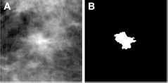
The size of each ROI is 512 x 512 pixels, which was extracted from the center of each identified suspicious mass lesion. We used a multilayer topographic region growth algorithm^9,38 to automatically segment the lesions. If there was noticeable segmentation error, the lesion boundary was corrected or re-drawn. Each lesion ROI was reduced or sub-sampled by a pixel averaging method using a kernel of 8 x 8 pixels in both x and y directions. The pixel size was thus increased from 50 x 50 μm in the original digitized image to 400 x 400 μm in the reduced image. Examples of a malignant mass and an FP detection from our dataset are displayed in Figures 1 and 2, respectively, along with their corresponding segmentations extracted by our mass segmentation scheme.

Figure 1.

Example of a malignant mass ROI (A) and its corresponding segmentation mask (B).

Figure 2.

example of an FP ROI (A) and its corresponding segmentation mask (B).

Methods

Neuroevolution

Neuroevolution methods use the evolutionary algorithms to train ANNs and can be divided into various groups based on the different encoding methods to optimize the connection weights and/or topology of the ANNs.⁴² With the fixed-topology neuroevolution systems,^43,44 the ANN topologies are fixed and only the node connection weights are evolved. Methods that evolve both the ANN weights and topologies are termed “topology and weight evolving artificial neural networks (TWEANNs).”^27,32,45 With TWEANNs, each individual in the population has a full specification with complete weight representation or information. Fitness evaluation is also accurate as there is a one-to-one mapping between the genotype and its phenotype.⁴² Another advantage of TWEANNs is that there is an option to start with minimal structure, and to increment structure only if there is an associated fitness improvement.

With TWEANNs, how to encode the individual genome is essential. The main issue associated with reproduction through the crossover process in TWEANNs is the competing conventions problem, also known as the permutations problem or variable length genome problem.⁴⁶ A systematic encoding system is required to ensure that there are no glitches in the evolutionary process, such as offspring genomes with the same structures being assigned to different innovation numbers or historical markings. Furthermore, a good encoding system will also ensure a more compact genome representation. Various types of encoding systems have been proposed in the literature.^47–52

NEAT is another recently developed neuroevolution method that has been proven effective in various applications and successfully solved the competing conventions problem in TWEANNs.^27,28 NEAT works through the process of complexification, namely the networks start with minimal topology, and structure is only incremented when it is found to improve or enhance network performance.³³ However, one of the pitfalls of NEAT is that feature selection is not enabled in NEAT. Feature selection is tremendously important as the exclusion of relevant features leads to suboptimal solutions, whereas the exclusion of irrelevant or redundant features adds unnecessary dimensions to the search space. In recent years, several variants of NEAT have been introduced and incorporated to feature selection or deselection (exclusion).^{26,31,53–55} For a more in-depth discussion on neuroevolution methods in the literature, the reader is referred to several literature reviews or surveys about the topic.^42,56

Phased searching with NEAT in a Time-Scaled Framework

In Ref. 26, Phased Searching with NEAT in a Time-Scaled Framework was presented and examined on 360 CT scans from the public Lung Image Database Consortium (LIDC) database. The method was shown to outperform the conventional NEAT in terms of sensitivity results, complexity of evolved networks, and evolution time.

Phased searching is based on the NEAT algorithm, which is distinct from other neuroevolution methods in three ways:²⁷ (1) crossover of different topologies is performed using innovation numbers as historical markings, (2) structural innovation is protected by speciation, and (3) incremental growth is performed from almost minimal structure. Phased searching outperforms NEAT in that it enables automatic feature selection or deselection on the input feature set, removes redundant structure, and also evolves simpler networks that are faster to be trained and validated in the evolutionary run.

With Phased Searching with NEAT in a Time-Scaled Framework, the search for useful network topologies is evolved in alternating between complexification and simplification phases.²⁶ During the complexification phases, useful structure (features, nodes, and connections) is added to the networks whereas during the simplification phases, redundant and irrelevant structure is discarded. Hence, the process of discarding redundant and irrelevant connections enables the search for optimal structure to proceed faster. For a detailed description of Phased Searching with NEAT in a Time-Scaled Framework, the reader is referred to Ref.^26.

In the previous work in Ref.²⁶, the complexification and simplification phases were implemented with equal generation numbers. In this study, we analyzed the performance of Phased Searching with equal and different generation numbers for the complexification or simplification phases. We implemented a new fitness function computed as the maximization of the area under the receiver operating characteristic (ROC) curve (AUC) on the training subsets. Namely, the network that maximized the AUC result on the training subset was selected, and subsequently applied to the testing subset. The computation of the fitness function as the maximization of the AUC is a proven criterion function as it has been analyzed and shown to perform well on other GA-based schemes or methods.^21,24

We also modified SharpNEAT 2.2.0,⁵⁷ which is a C# implementation of NEAT, to implement Phased Searching with NEAT in a Time-Scaled Framework. We also performed the training and validation of our mass detection scheme using a 10-fold cross-validation method, the details of which are provided in the Experimental Setup and Classification Methodology section. In any GA process, several runs on the training subsets have to be repeated to perform a global search over the search space for the optimal network before the trained network is applied on the testing subsets. We selected the network that maximized the AUC result on the training subset over five runs. This process was repeated 10 times for the 10 different training subsets using our 10-fold cross-validation method (namely, five runs for each training subset, repeated 10 times for the 10 individual subsets).

Feature computation

In this study, we computed 271 image features for our mass detection scheme on all 1,600 ROIs of our database. The top-level block diagram of our mass detection scheme is displayed in Figure 3. The computed features are based on shape, spiculation, texture, contrast, isodensity, presence and location of fat, and/or calcifications. We also included 27 previously computed features for mass detection in our previous studies.^9,39 A summary of the computed features is provided in Table 1. In this section, we present a brief overview of these features; for their detailed description, the reader is referred to Ref.^58.

Figure 3.

A flow diagram of our mass detection scheme.

Table 1

summary of computed image features for our mass detection scheme.

FEATURE GROUP/TYPE	DESCRIPTION
Shape	Eccentricity, equivalent diameter, extent, convex area, major axis length, minor axis length, orientation, solidity, shape factor ratio, ratio of major to minor axis length, modified compactness
Fat	Size (pixel number), size factor ratio (size/mass area), region number, average distance to the mass center (average distance/mean radial length of mass region)
Calcifications	Size (pixel number), size factor ratio (size/mass area), region number
Texture (lesion segment only)	4 gray level co-occurrence matrix based features, 22 average and maximum values of gray level run length based texture features
Texture (dilated lesion segments)	24 average and maximum values of gray level co-occurrence matrix based features, 66 average and maximum values of gray level run length based texture features
Spiculation	Features computed on the maxima points and on the whole image of the divergence of the normalized gradient (DNG) and the curl of the normalized gradient (CNG)
Contrast	Contrast based features (previously defined in Refs.^8,9,64) computed for different-sized regions and locations of the lesion segments and background
Isodensity	Isodensity based features (previously defined in Ref.⁸) computed for different-sized regions and locations of the lesion segments and background
Previously-computed features	27 intensity, contrast, shape, border segment, and local topology based features previously described in refs.^9,39,65

Various shape features have been proposed in the literature for mass detection or classification.^7,11,14 We computed a mixture of novel and previously proposed shape features as listed in Table 1. The modified compactness^59,60 and shape factor ratio^61,62 are the most common and established shape features that have appeared in the literature. For a full description of the shape features, the reader is referred to Refs.^58,63.

We proposed four fat-related features to determine the presence and location of fat within the segmented lesions. First, we applied an empirically determined threshold of 2,600 to extract the fat regions within the lesion segments. Then, we computed four features on the extracted fat regions: area, ratio of the fat area to the lesion segment area, number of fat regions within the mass (the fat regions were segmented by eight-connected-component labeling), and the average distance between the centroids of the segmented fat regions and the centroid of the whole lesion segment. We also computed three features to detect the presence of calcifications within the lesion segments, which are listed in Table 1 and are self-explanatory.

In the literature, many studies have proposed various texture features for mass detection or classification.¹¹ We computed some previously determined features (22 gray-level run length and 4 gray-level co-occurrence matrix-based features) on original (undilated) lesion segments. On dilated lesion segments, we computed 24 average and maximum values of gray-level co-occurrence matrix-based features, and 66 average and maximum values of gray-level run length-based texture features.

We have also computed some spiculation features on the lesion segments based on the divergence of the normalized gradient (DNG) and the curl of the normalized gradient (CNG). If an FP ROI is modeled as a circular region with homogeneous intensity against a darker background, the computation of the DNG feature should produce a maximum value at the location of its center point. On the other hand, the computation of the CNG feature will produce a high result at the location of the center point of a spicular region. We computed altogether 20 spiculation-based features (including mean, maximum, minimum, standard deviation, and median of the CNG and DNG, and the same statistical features computed on the maxima points located near the center regions of the lesion segments), on Gaussian-blurred images of the lesion segments.

In Ref.⁵⁸ we presented a novel approach of computing four previously determined contrast measures^8,62,64 over differently predefined inner and outer regions of the lesion segments. Our approach differs from previous approaches in that we compute the contrast features over different-sized regions of the lesion and over different regions of the lesion background. This approach is based on our observation that different inner regions of the lesion have different structural appearances and intensities eg, pixels immediately adjacent to the mass contour frequently have a different structure and appearance from the pixels near the center of the mass region. Additionally, different regions of the lesion background have a different structural appearance ie the pixel intensities near the lesion contour are slightly higher than the pixel intensities further away.

To compute the contrast-based features, we extracted the outer region (O), by dilating the lesion segment with fat, disk-shaped, or “disc” structuring elements (SEs) of three different sizes: (1) mean radial length of the mass, (2) 1/2 of the mean radial length, and (3) 1/4 of the mean radial length, whereby the mean radial length was defined previously.⁶¹ We also defined the inner region of the lesion (I) by the whole inner segment of the lesion within its contour, and also defined two other regions of the lesion by performing an erosion operation on I. To obtain the other two inner segments, we performed an erosion operation on I using a “disc” SE of three different sizes: (1) mean radial length of the mass, (2) 1/2 of the mean radial length, and (3) 1/4 of the mean radial length. After the erosion operation, we obtained the eroded image denoted by I₁, and the resultant image by subtracting I ₁ from I, denoted by I ₂. Thus, the new contrast-based features were computed between the inner and outer regions of the mass (between O and I, O and I ₁, and O and I ₂). In this way, we computed altogether 5 x 3 x 4 = 60 contrast-based features per lesion segment.

Finally, we computed 27 ROI morphological features that were defined in our previous publications.^9,39,65 These features consisted of different intensities, contrasts, shapes, border segments, and local topological-based features.

Performance comparisons with other classifiers

To assess Phased Searching's performance, we performed performance comparisons with other well-established classifiers for the mass detection task, namely fixed-topology ANNs, SVMs, bagged decision trees, and LDA. The parameter tuning for each classifier was performed on the training subsets that were kept completely separated from the testing subsets.

First, we trained and optimized a LIBSVM classifier⁶⁶ with the radial basis function (RBF) kernel, defined as K(x_i,x^j) = exp(-γ||x_i–x_j||²), γ > 0, on the training set of instance-label pairs (x_i, y_i), i = 1, …, l, where x_i ∈ R_n and $y_{i} \in {1, - 1}, \forall i = 1, \dots, l$ . A recommended five-fold cross-validation method with a parallel “grid-search”⁶⁷ was used to determine the penalty parameter of the error term and γ.

Second, we analyzed a standard feed-forward ANN with a single hidden layer and with a hyperbolic tangent activation function at the hidden nodes, and a linear activation function at the output node (default parameters in the Matlab® Neural Network toolbox). The number of input nodes was equal to the number of features (271). The fixed-topology ANN was trained by a backpropagation algorithm whereby the network's performance was analyzed for 2–40 nodes in the hidden layer (using the AUC computed on the training set as the performance measure), which was always initialized with random weights.

Third, the LDA and decision tree classifiers are also popular and used for mass detection.^11,68–72 We included them in our study. Bagged decision trees are an ensemble of classification trees, and in initial experiments, they gave a better response than the single decision tree with binary splits for classification. The LDA classifier is a traditional classification method that has a high performance for linearly separable problems; however, it might adapt poorly for non-linear separable data.

The input features were linearly normalized (between 0 and 1) for the SVM, fixed-topology ANN, and Phased Searching classifiers. For LDA and bagged decision trees, normalization of the input features did not affect the classifier outcomes, and was thus omitted.

Experimental setup and classification methodology

Training and validation of our mass detection scheme was performed in a 10-fold cross-validation framework. In this method, the 800 malignant true-positive (TP) ROIs and 800 FP ROIs were randomly segmented into 10 exclusive subsets. Classifier training was then performed on nine TP and nine FP subsets, with the remaining one TP subset and one FP subset used for testing. This process was repeated iteratively using the different combinations of the nine TP and nine FP subsets each time so that each of the TP and FP ROIs was tested once with a classifier-generated probability score. Finally, the results on all 10 testing subsets were averaged and used to generate a ROC curve. By averaging the results on the 10 testing subsets, we can obtain the mean and standard deviation intervals at specific points on the ROC curve.

We also computed the AUCs of each examined classifier, and performed statistical significance tests on the obtained results. Furthermore, we performed an analysis on the features selected by Phased Searching in terms of frequency of selection per feature grouping/type. This analysis is important to examine the features that were beneficial for Phased Searching, and were thus included in the learning process and throughout the evolutionary run(s).

We performed an analysis of varying the alternating complexification and simplification parameter values of Phased Searching. In the original study performed on 360 lung CT scans from the LIDC database,²⁶ Phased Searching was examined only for equal values of the alternating complexification or simplification phases or cycles. Thus, in this study, we analyzed Phased Searching's performance for equal and unequal values of the complexification and simplification phases. We performed the following analysis on the networks evolved by Phased Searching: (1) best fitness per generation, (2) complexity (number of connections) of the best network per generation, and (3) average network complexity per generation. The AUCs obtained by varying the complexification or simplification parameters are tabulated.

Results

The computed ROC curves for all analyzed classifiers are displayed in Figure 4. We also computed and tabulated the average AUC results with standard deviation intervals over the 10 folds of each classifier in Table 2. The results indicate that SVM, fixed-topology ANNs, and Phased Searching outperform the bagged decision trees and LDA classifiers. The SVM classifier slightly outperformed the ANN and Phased Searching classifiers.

Figure 4.

ROC curves of the five compared classifiers computed over the 10-fold cross-validation experiments–(1) Phased searching with neat in a time-scaled framework using the maximization of AUC as the fitness function, (2) fixed-topology ANNs, (3) SVMs, (4) bagged decision trees, and (5) LDA. The error bars are symmetric, and are two standard deviation units in length.

Table 2

Average AUC values and the corresponding standard deviations for the five compared classifiers computed using the 10-fold cross-validation experiments.

METHOD	AUC
Phased searching	0.856 ± 0.029
ANN	0.871 ± 0.025
SVM	0.886 ± 0.026
Decision trees	0.807 ± 0.015
LDA	0.841 ± 0.028

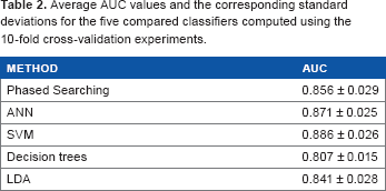
Table 3 displays the P-values comparing the AUC results of the different classifiers. In Table 3, the diagonal P-values are equivalent and thus omitted. It shows that Phased Searching outperforms the bagged decision trees and LDA classifiers, and the difference in the AUC results is statistically significant for bagged decision trees (P, 0.001), but not for LDA (P = 0.270). SVM outperforms Phased Searching with a statistical significance (P = 0.026). Fixed-topology ANNs slightly outperform Phased Searching, but the difference is not statistically significant (P = 0.242). SVM also outperforms fixed-topology ANNs, but it is not statistically significant (P = 0.196). LDA is significantly outperformed by ANN (P = 0.024) and SVM (P = 0.002).

Table 3

Student's t-test performed at the 5% significance level to study if the AUC results of the different classifiers are significantly different from each other. The P-value of rejecting the null hypothesis is given in the table. The diagonal P-values in the table are equivalent; thus, they have been omitted (–).

METHOD	P-VALUE PHASED SEARCHING	ANN	SVM	DECISION TREES	LDA
Phased searching	–	0.242	0.026	<0.001	0.270
ANN	–	–	0.196	<0.001	0.024
SVM	–	–	–	<0.001	0.002
Decision trees	–	–	–	–	0.004
LDA	–	–	–	–	–

Table 4 shows the distributions of the features selected or retained by Phased Searching at the end of the evolutionary runs. The middle column of Table 4 shows the number of features in each group (eg, there are 4 fat-related features out of 271 total features). The far-right column thus displays the percentage of features that were retained in the group and their standard deviation intervals computed over the 10-fold cross-validation experiments. For example, 80.0% of the fat-related features (80.0% x 4 = 3.2 features) were retained by Phased Searching with a standard deviation interval of 23.0% or 0.92 features.

Table 4

features selected or retained by Phased searching with neat in a time-scaled framework. The 271 proposed features are divided into nine feature groups or types listed in the far-left column. The number of the features represented in each group is represented in the middle column. The average percentages of the features selected by Phased searching with standard deviation intervals are shown in the far-right column.

FEATURE GROUP/TYPE	NUMBER OF FEATURES	AVERAGE PERCENTAGE AND STD. DEV. INTERVALS
Shape	11	77.3 ± 13.0%
Fat	4	80.0 ± 23.0%
Calcifications	3	80.0 ± 17.2%
Texture (mass segment only)	26	68.1 ± 10.1%
Texture (dilated mass segments)	90	75.4 ± 5.0%
Spiculation	20	65.5 ± 13.8%
Contrast	60	75.8 ± 5.6%
Previously-computed morphological features	27	74.1 ± 7.4%
Isodensity	30	28.3 ± 4.8%

Figures 5–7 display the results of the analysis performed as the change of complexification and simplification parameters selected in Phased Searching algorithm. The figures display the average and standard deviation intervals of the best fitness, complexity of the best network, and average network complexity, respectively, of the networks evolved over the 10-fold cross-validation experiments. The AUC results corresponding to the performed parameter analysis are tabulated in Table 5.

Figure 5.

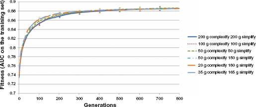
Graphs of the fitness computed as the AUC of the training subsets of the best network per generation in the run of the best-performing network (selected out of five runs), averaged on the 10 folds of Phased Searching with NEAT in a Time-Scaled Framework with alternating generations of complexification or simplification phases.

Figure 6.

Graphs of the number of connections of the best network per generation in the run of the best-performing network (selected out of five runs), averaged on the 10 folds of Phased Searching with NEAT in a Time-Scaled Framework with alternating generations of complexification or simplification phases.

Figure 7.

Graphs of the average network complexity (average number of connections) per generation in the run of the best-performing network (selected out of five runs), averaged on the 10 folds of Phased Searching with NEAT in a Time-Scaled Framework with alternating generations of complexification or simplification phases.

Table 5

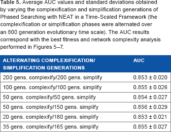
average AUC values and standard deviations obtained by varying the complexification and simplification generations of Phased searching with neat in a time-scaled framework (the complexification or simplification phases were alternated over an 800 generation evolutionary time scale). The AUC results correspond with the best fitness and network complexity analysis performed in Figures 5–7.

ALTERNATING COMPLEXIFICATION/SIMPLIFICATION GENERATIONS	AUC
200 gens. complexify/200 gens. simplify	0.853 ± 0.020
100 gens. complexify/100 gens. simplify	0.855 ± 0.026
50 gens. complexify/50 gens. simplify	0.854 ± 0.027
50 gens. complexify/150 gens. simplify	0.856 ± 0.029
20 gens. complexify/180 gens. simplify	0.853 ± 0.021
35 gens. complexify/165 gens. simplify	0.855 ± 0.027

Discussion

The results show that Phased Searching outperformed bagged decision trees and LDA in the classification task, and its performance was not significantly different from the ANN classifier (P = 0.242). SVM produced the best performance among all the classifiers analyzed, and significantly outperformed Phased Searching at the 5% significance level (P = 0.026). This result is somehow unexpected. We had initially expected that the number of input features (271) was too large for the task at hand, and that Phased Searching's ability to select relevant features during the complexification phases and discard (deselect) irrelevant and redundant features during the simplification phases would give it an advantage over the other classifiers. The results indicate, however, that the inclusion of the 271 features was beneficial for the classifiers analyzed, especially for the fixed-topology ANN and SVM classifiers.

Another advantage of the SVM classifier over ANNs is that it is a maximum margin classifier, namely it minimizes the classification error and maximizes the geometric margin simultaneously. In doing so, unlike ANNs, SVM does not suffer from “overfitting” on the training sets. Phased Searching, which is an ANN-based classifier, can thus also be affected by “overfitting.” Furthermore, as Phased Searching relies entirely on GAs during the training and evolution processes, the GA algorithm enables it to search globally optimal solutions; however, its performance might be affected by the lack of a refinement procedure (such as backpropagation training).⁴²

Although Phased Searching was outperformed by SVM, it performed better than the LDA and decision tree classifiers, both of which are widely used and are highly popular for mass detection.^11,68–72 Furthermore, Phased Searching's overall performance is comparable with and simultaneously uses fewer features than fixed-topology ANNs. Although it is slightly outperformed by SVM, it requires the computation of fewer features, which reduces the computational time requirement at the feature computation stage, and also reduces the overall training and validation time requirement of the mass detection scheme.

The results of the analysis of features selected by Phased Searching at the end of 800 generations show that the fat, calcification, and shape-related features were most frequently selected or retained by Phased Searching. The isodensity and spiculation features were the least frequently selected features.

The results of analyzing the complexification or simplification parameters in Table 5 and in Figures 5–7 show that varying these parameters only produced a small change in the AUC results of Phased Searching. The highest AUC result of 0.856 ± 0.029 was obtained from an experiment involving 50 generations of complexification and 150 generations of simplification, which indicates that those were the best parameters for the classification task at hand.

This outcome cannot be ultimately predicted from the analysis performed on the fitness of the best networks evolved for more than 800 generations in Figure 5, as the graphs for the unequal complexification or simplification runs overlap too closely. However, in Figures 6 and 7, namely the analysis of the best network and average network complexities, we observe that the network complexities in the experiment involving the 50 complexification and 150 simplification generations stabilized at a fixed value or range at the end of 800 generations. For the experiments of equal complexification and simplification generations (ie, 200, 100, and 50), the average and the best network complexities displayed an increasing trend, and continued to increase at the end of 800 generations. This trend in the network complexities was also observed in the original experiments that analyzed Phased Searching's performance in a lung nodule detection task, which was conducted solely with equal complexification and simplification phases.²⁶

The average and the best network complexities obtained for the other two experiments conducted with unequal complexification or simplification generations (namely, 35 complexification or 165 simplification generations, and 20 complexification or 180 simplification generations) in Figures 6 and 7 show that unlike the experiment with a mix of 50 complexification and 150 simplification generations, the network complexities gradually decreased and did not stabilize at the end of 800 generations for these two experiments. The results in Figures 5–7 and the corresponding AUC results in Table 5 indicate that the optimal network topologies (connections and nodes) were evolved for the 50 complexification and 150 simplification generation parameter values, which produced the best network and average network complexities to evolve and stabilize the classification task at hand.

Although this study demonstrates promising results, it is rather preliminary and has a number of limitations. For example, this is a laboratory-based technology development study using a testing dataset with an equal number of positive to negative images, which does not represent the actual cancer prevalence ratio in general breast screening practice. Also, as a relatively small image testing dataset, the potential case selection bias might exist making it unable to fully represent the diversity in the general breast cancer screening population. Therefore, the robustness of this new approach and our new scheme needs to be further validated using the large and diverse image databases in future studies.

Conclusions

We conducted experiments to analyze a new GA-based classifier, Phased Searching with NEAT in a Time-Scaled Framework in a challenging computer-aided mass detection task, and compared its performance with several other well-established classifiers in the field. Phased Searching achieved an AUC result of 0.856 ± 0.029, and significantly outperformed a bagged decision tree classifier (P, 0.001), and slightly outperformed an LDA classifier (P = 0.270). Phased Searching was only significantly outperformed by the SVM classifier (P = 0.026), and performed comparably with the fixed-topology ANN classifier (P = 0.242). The highest AUC result was achieved in this task by the SVM classifier (AUC = 0.886 ± 0.026). Analysis performed on the network complexities evolved by Phased Searching indicates that it can evolve optimal network topologies provided that its complexification and simplification parameters are optimally chosen, as it produced AUC results that are comparable to the state-of-the-art classifiers, but with fewer number of features being selected, and thus a lower training and validation time requirement. From this study, it can also be concluded that the three classifiers, namely SVM, fixed-topology ANN, and Phased Searching with NEAT in a Time-Scaled Framework, are performing comparably well in our computer-aided mammographic mass detection scheme.

Author Contributions

MT, JP, and BZ conceived and designed the experiments. MT analyzed the data. MT wrote the first draft of the manuscript. MT and BZ contributed to the writing of the manuscript. MT, JP, and BZ agreed with manuscript results and conclusions. MT and BZ jointly developed the structure and arguments for the paper. MT, J P, and BZ made critical revisions and approved the final version. All authors reviewed and approved the final manuscript.

Supplementary Data

The parameters are based on SharpNEAT 2.2.0,⁵⁷ and remained constant throughout the evolutionary run. The best parameter values were obtained on the training subsets of the 10-fold cross-validation experiments, which were kept completely separated from the testing subsets:

Population number (number of genomes/networks): 200

Species number: 10

Number of generations (per run): 800

Connection weight range: {-0.05, 0.05}. This parameter gets or sets the connection weight range to use in the genomes eg, a value of 5 defines a weight range of -5 to 5. The weight range is strictly enforced ie when creating new connections and mutating existing ones.

Probability that all the excess and disjoint genes were copied into an offspring genome during sexual reproduction: 0

Interspecies mating rate: 0.01

Elitism proportion: 0.2. The species genomes are first sorted by fitness. The top N% are kept, whereas the other genomes are removed to make way for the offspring.

Selection proportion: 0.2. The species genomes are first sorted by fitness. Then, the parent genomes are selected for producing offspring from the top N%. Selection is performed before elitism is applied, thus selecting from more genomes than will be made elite is possible.

We also used the hyperbolic tangent activation function at the hidden nodes and a modified sigmoidal activation function²⁷ at the output node.

The following parameter values were used only during the complexification phases:

Probability of adding a new node: 0.15

Probability of adding a new connection: 0.35

Connection weight mutation probability: 0.5

Probability that a genome mutation was a “delete connection” mutation: 0.001

Proportion of offspring from asexual reproduction (mutation): 0.8

Proportion of offspring from sexual reproduction (crossover): 0.2

These parameter values follow a logical pattern eg, connections (links) need to be added more often than nodes. The following parameter values were used only during the simplification phases:

Connection weight mutation probability: 0.6

Probability that a genome mutation was a “delete connection” mutation: 0.4

Proportion of offspring from asexual reproduction (mutation): 1

Proportion of offspring from sexual reproduction (crossover): 0.

References

American Cancer Society. What are the Key Statistics About Breast Cancer? 2014. http://www.cancer.org/cancer/breastcancer/detailedguide/breast-cancer-key-statistics.

Tabar

, Vitak

, Chen

H.H.

, Yen

M.F.

, Duffy

S.W.

, Smith

R.A.

. Beyond randomized controlled trials: organized mammographic screening substantially reduces breast carcinoma mortality. Cancer. 2001; 91(9): 1724–31.

Smith

R.A.

, Cokkinides

, Brooks

, Saslow

, Shah

, Brawley

O.W.

. Cancer screening in the United States, 2011: a review of current American Cancer Society guidelines and issues in cancer screening. CA Cancer J Clin. 2011; 61(1): 8–30.

American Cancer Society. ACR BI-RADS—Mammography, Ultrasound & Magnetic Resonance Imaging, 4th ed. Reston, VA: American College of Radiology; 2003.

Morton

M.J.

, Whaley

D.H.

, Brandt

K.R.

, Amrami

K.K.

. Screening mammograms: interpretation with computer-aided detection—prospective evaluation. Radiology. 2006; 239(2): 375–83.

Brem

R.F.

, Baum

, Lechner

. Improvement in sensitivity of screening mammography with computer-aided detection: a multiinstitutional trial. AJR Am J Roentgenol. 2003; 181(3): 687–93.

Oliver

, Freixenet

, Martí

. A review of automatic mass detection and segmentation in mammographic images. Med Image Anal. 2010; 14(2): 87–110.

Brake

G.M.T.

, Karssemeijer

, Hendriks

J.H.

. An automatic method to discriminate malignant masses from normal tissue in digital mammograms. Phys Med Biol. 2000; 45(10): 2843–57.

Zheng

, Chang

Y-H

, Gur

. Computerized detection of masses in digitized mammograms using single-image segmentation and a multilayer topographic feature analysis. Acad Radiol. 1995; 2(11): 959–66.

10.

Wei

, Sahiner

, Hadjiiski

L.M.

. Computer-aided detection of breast masses on full field digital mammograms. Med Phys. 2005; 32(9): 2827–38.

11.

Cheng

H.D.

, Shi

X.J.

, Min

, Hu

L.M.

, Cai

X.P.

, Du

H.N.

. Approaches for automated detection and classification of masses in mammograms. Pattern Recognit. 2006; 39(4): 646–68.

12.

Campanini

, Dongiovanni

, Iampieri

. A novel featureless approach to mass detection in digital mammograms based on support vector machines. Phys Med Biol. 2004; 49(6): 961–75.

13.

Zheng

, Chang

Y-H

, Wang

X.H.

, Good

W.F.

, Gur

. Application of a Bayesian belief network in a computer-assisted diagnosis scheme for mass detection. Proc SPIE. 1999; 3661: 1553–61.

14.

Rangayyan

R.M.

, Ayres

F.J.

, Desautels

J.E.L.

. A review of computer-aided diagnosis of breast cancer: toward the detection of subtle signs. J Franklin Inst. 2007; 344(3-4): 312–48.

15.

Horsch

A.H.

, Hapfelmeier

, Elter

. Needs assessment for next generation computer-aided mammography reference image databases and evaluation studies. Int J Comput Assist Radiol Surg. 2011; 6(6): 749–67.

16.

Sahiner

, Chan

H.P.

, Petrick

. Classification of mass and normal breast tissue: a convolution neural network classifier with spatial domain and texture images. IEEE Trans Med Imaging. 1996; 15(5): 598–610.

17.

Zheng

, Sumkin

J.H.

, Zuley

M.L.

, Lederman

, Wang

, Gur

. Computer-aided detection of breast masses depicted on full-field digital mammograms: a performance assessment. Br J Radiol. 2012; 85: e153–61.

18.

Huo

, Giger

M.L.

, Vyborny

C.J.

, Wolverton

D.E.

, Metz

C.E.

. Computerized classification of benign and malignant masses on digitized mammograms: a study of robustness. Acad Radiol. 2000; 7(12): 1077–84.

19.

, Nandi

A.K.

, Rangayyan

R.M.

. Classification of breast masses using selected shape, edge-sharpness, and texture features with linear and kernel-based classifiers. J Digit Imaging. 21(2) 2009: 153–69.

20.

Mavroforakis

, Georgiou

, Dimitropoulos

, Cavouras

, Teodoridis

. Significance analysis of qualitative mammographic features, using linear classifiers, neural networks and support vector machines. Eur J Radiol. 2005; 54(1): 80–9.

21.

Zheng

, Chang

Y-H

, Wang

X.H.

, Good

W.F.

, Gur

. Feature selection for computerized mass detection in digitized mammograms by using a genetic algorithm. Acad Radiol. 1999; 6(6): 327–32.

22.

Sahiner

, Chan

H.P.

, Petrick

, Helvie

M.A.

, Goodsitt

M.M.

. Design of a high-sensitivity classifier based on a genetic algorithm: application to computer-aided diagnosis. Phys Med Biol. 1998; 43(10): 2853–71.

23.

Campanini

, Lanconelli

. Genetic algorithms in CAD mammography. Proc SPIE. 2006; 6515: 129–57.

24.

Mazurowski

M.A.

, Habas

P.A.

, Zurada

J.M.

, Tourassi

G.D.

. Decision optimization of case-based computer-aided decision systems using genetic algorithms with application to mammography. Phys Med Biol. 2008; 53(4): 895–908.

25.

Zheng

, Chang

Y-H

, Good

W.F.

, Gur

. Performance gain in computer-assisted detection schemes by averaging scores generated from artificial neural networks with adaptive filtering. Med Phys. 2001; 28(11): 2302–8.

26.

Tan

, Deklerck

, Cornelis

, Jansen

. Phased searching with NEAT in a time-scaled framework: experiments on a computer-aided detection system for lung nodules. Artif Intell Med. 2013; 59(3): 157–67.

27.

Stanley

K.O.

, Miikkulainen

. Evolving neural networks through augmenting topologies. Evol Comput. 2002; 10(2): 99–127.

28.

Stanley

K.O.

, Bryant

B.D.

, Miikkulainen

. Real-time neuroevolution in the NERO video game. IEEE Trans Evol Comput. 2005; 9(6): 653–68.

29.

Gomez

, Miikkulainen

. Incremental evolution of complex general behavior. Adapt Behav. 1997; 5(3-4): 317–42.

30.

Igel

. Neuroevolution for reinforcement learning using evolution strategies. Paper presented at: Congress on Evolutionary Computation; December 8–12, 2003. Canberra, Australia.

31.

Tan

, Hartley

, Bister

, Deklerck

. Automated feature selection in neuroevolution. Evol Intell. 2009; 4(1): 271–92.

32.

Stanley

K.O.

. Efficient Evolution of Neural Networks Trough Complexification [PhD thesis]. The University of Texas at Austin; 2004. Austin, TX, USA.

33.

Stanley

K.O.

, Miikkulainen

. Competitive coevolution through evolutionary complexification. J Artif Intell Res. 2004; 21: 63–100.

34.

Clune

, Stanley

K.O.

, Pennock

R.T.

, Ofria

. On the performance of indirect encoding across the continuum of regularity. IEEE Trans Evol Comput. 2011; 15(3): 346–67.

35.

Stanley

K.O.

, D'Ambrosio

D.B.

, Gauci

. A hypercube-based encoding for evolving large-scale neural networks. Artif Life. 2009; 15(2): 185–212.

36.

Tan

, Deklerck

, Jansen

, Bister

, Cornelis

. A novel computer-aided lung nodule detection system for CT images. Med Phys. 2011; 38(10): 5630–45.

37.

Tan

, Deklerck

, Jansen

, Cornelis

. Analysis of a feature-deselective neuroevolution classifier (FD-NEAT) in a computer-aided lung nodule detection system for CT images. In: Proceedings of the 14th International Conference on Genetic and Evolutionary Computation (GECCO) Conference Companion; 2012; Philadelphia, PA.

38.

Gur

, Stalder

J.S.

, Hardesty

L.A.

. Computer-aided detection performance in mammographic examination of masses: assessment. Radiology. 2004; 233(2): 418–23.

39.

Zheng

, Lu

, Hardesty

L.A.

. A method to improve visual similarity of breast masses for an interactive computer-aided diagnosis environment. Med Phys. 2006; 33(1): 111–7.

40.

Park

S.C.

, Wang

X.H.

, Zheng

. Assessment of performance improvement in content-based medical image retrieval schemes using fractal dimension. Acad Radiol. 2009; 16(10): 1171–8.

41.

Zheng

, Leader

J.K.

, Abrams

. Computer-aided detection schemes: the effect of limiting the number of cued regions in each case. Am J Roentgenol. 2004; 182(3): 579–83.

42.

Yao

. Evolving artificial neural networks. Proc IEEE. 1999; 87(9): 1423–47.

43.

Saravanan

, Fogel

D.B.

Evolving neural control systems,

IEEE Intelligent Systems 1995; 10: 23–7.

44.

Gomez

F.J.

, Miikkulainen

. Solving non-Markovian control tasks with neuroevolution. Paper presented at: International Joint Conference on Artificial Intelligence; 1999; Stockholm, Sweden.

45.

Gruau

, Whitley

, Pyeatt

. A comparison between cellular encoding and direct encoding for genetic neural networks. In: Proceedings of the 1st Annual Conference on Genetic Programming; eds Koza JR, Goldberg DE, Fogel DB, Riolo RL; Cambridge, MA; 1996: 81–9.

46.

Radcliffe

N.J.

. Genetic set recombination and its application to neural network topology optimisation. Neural Comput Appl. 1993; 1(1): 67–90.

47.

Dasgupta

, McGregor

. Designing application-specific neural networks using the structured genetic algorithm. In: Proceedings of the International Conference on Combinations of Genetic Algorithms and Neural Networks; publish is IEEE Xplore. Baltimore, MD, USA. 1992: 87–96.

48.

Janson

D.J.

, Frenzel

J.F.

. Training product unit neural networks with genetic algorithms. IEEE Expert. 1993; 8: 26–33.

49.

Gruau

. Genetic synthesis of modular neural networks. In: Proceedings of the 5th International Conference on Genetic Algorithms; 1993: 318–25.

50.

Dolan

C.P.

, Dyer

M.G.

. Toward the evolution of symbols. In: Int. Conf. Genetic Algorithms and their Applications; Hillsdale, NJ: Erlbaum; 1987: 123–31.

51.

Pujol

J.C.F.

, Poli

. Evolution of the topology and the weights of neural networks using genetic programming with a dual representation. Technical Report CSRP-97–7. Birmingham, UK: School of Computer Science, The University of Birmingham; 1997.

52.

Angeline

P.J.

, Saunders

G.M.

, Pollack

J.B.

. An evolutionary algorithm that constructs recurrent neural networks. IEEE Trans Neural Networks. 1993; 5: 54–65.

53.

Whiteson

, Stanley

K.O.

, Mikkulainen

. Automatic feature selection in neuroevolution. In: Proceedings of Genetic and Evolutionary Computation Conference (GECCO) Workshop Program; 2004; New York, NY.

54.

Loscalzo

, Wright

, Acunto

, Yu

. Sample aware embedded feature selection for reinforcement learning. In: Proceedings of Genetic and evolutionary computation conference (GECCO); Philadelphia, PA: ACM; 2012: 887–94.

55.

Green

. Phased searching with NEAT: alternating between complexification and simplification. Technical Report. 2004.

56.

Floreano

, Dürr

, Mattiussi

. Neuroevolution: from architectures to learning. Evol Intell. 2008; 1(1): 47–62.

57.

SharpNEAT 2.2.0. http://sourceforge.net/projects/sharpneat/. 2013. Accessed December 16, 2013.

58.

Tan

, Pu

, Zheng

. Optimization of breast mass classification using sequential forward floating selection (SFFS) and a support vector machine (SVM) model. Int J CARS. 2014. DOI 10.1007/s11548-014-0992-1.

59.

Rangayyan

R.M.

, El-Faramawy

N.M.

, Desautels

J.E.

, Alim

O.A.

. Measures of acutance and shape for classification of breast tumors. IEEE Trans Med Imaging. 1997; 16(6): 799–810.

60.

Shen

, Rangayyan

R.M.

, Desautels

J.E.L.

. Detection and classification of mammographic calcifications. Int J Pattern Recognit Artif Intell. 1993; 7(6): 1403–16.

61.

Kilday

, Palmieri

, Fox

M.D.

. Classifying mammographic lesions using computerized image analysis. IEEE Trans Med Imaging. 1993; 12(4): 664–9.

62.

Zheng

, Leader

J.K.

, Abrams

G.S.

. Multiview-based computer-aided detection scheme for breast masses. Med Phys. 2006; 33(9): 3135–43.

63.

Tan

, Pu

, Zheng

. A new mass classification system derived from multiple features and a trained MLP model. In: Proc. SPIE (Medical Imaging 2014: Computer-Aided Diagnosis); February 12, 2014; San Diego, CA.

64.

Varela

, Timp

, Karssemeijer

. Use of border information in the classification of mammographic masses. Phys Med Biol. 2006; 51: 425–41.

65.

Zheng

, Wang

, Lederman

, Tan

, Gur

. Computer-aided detection; the effect of training databases on detection of subtle breast masses. Acad Radiol. 2010; 17(11): 1401–8.

66.

Chang

C-C

, Lin

C-J

. LIBSVM: a library for support vector machines. ACM TIST. 2011; 2(3): 27.

67.

Hsu

C-W

, Chang

C-C

, Lin

C-J

. A practical guide to support vector classification. Technical Report. National Taiwan University, Taipei 106, Taiwan; 2009. Taipei, Taiwan.

68.

Sahiner

, Petrick

, Chan

H.P.

. Computer-aided characterization of mammographic masses: accuracy of mass segmentation and its effects on characterization. IEEE Trans Med Imaging. 2001; 20(12): 1275–84.

69.

Bruce

L.M.

, Adhami

R.R.

. Classifying mammographic mass shapes using the wavelet transform modulus-maxima method. IEEE Trans Med Imaging. 1999; 18(12): 1170–7.

70.

Petrick

, Chan

H.P.

, Wei

, Sahiner

, Helvie

M.A.

, Adler

D.D.

. Automated detection of breast masses on mammograms using adaptive contrast enhancement and texture classification. Med Phys. 1996; 23(10): 1685–96.

71.

Zheng

, Chan

A.K.

. An artificial intelligent algorithm for tumor detection in screening mammogram. IEEE Trans Med Imaging. 2001; 20(7): 559–67.

72.

, Qian

, Clarke

L.P.

, Clark

R.A.

, Tomas

J.A.

. Improving mass detection by adaptive and multiscale processing in digitized mammograms. Proc SPIE. 1999; 3661: 490–8.

Optimization of Network Topology in Computer-Aided Detection Schemes Using Phased Searching with NEAT in a Time-Scaled Framework

Abstract

Keywords

Introduction

Materials/Dataset

Methods

Neuroevolution

Phased searching with NEAT in a Time-Scaled Framework

Feature computation

Performance comparisons with other classifiers

Experimental setup and classification methodology

Results

Discussion

Conclusions

Author Contributions

Supplementary Data

References