Sage Journals: Discover world-class research

Abstract

Gene set enrichment analysis (GSA) methods have been widely adopted by biological labs to analyze data and generate hypotheses for validation. Most of the existing comparison studies focus on whether the existing GSA methods can produce accurate P-values; however, practitioners are often more concerned with the correct gene-set ranking generated by the methods. The ranking performance is closely related to two critical goals associated with GSA methods: the ability to reveal biological themes and ensuring reproducibility, especially for small-sample studies. We have conducted a comprehensive simulation study focusing on the ranking performance of seven representative GSA methods. We overcome the limitation on the availability of real data sets by creating hybrid data models from existing large data sets. To build the data model, we pick a master gene from the data set to form the ground truth and artificially generate the phenotype labels. Multiple hybrid data models can be constructed from one data set and multiple data sets of smaller sizes can be generated by resampling the original data set. This approach enables us to generate a large batch of data sets to check the ranking performance of GSA methods. Our simulation study reveals that for the proposed data model, the Q2 type GSA methods have in general better performance than other GSA methods and the global test has the most robust results. The properties of a data set play a critical role in the performance. For the data sets with highly connected genes, all GSA methods suffer significantly in performance.

Keywords

gene set enrichment analysis feature ranking data model simulation study

Background

Gene expression microarray analysis is now routinely performed in biology labs to profile the transcriptional activity of target sample cells. This mature technique provides a cost-effective way to conduct a preliminary study on a small cohort to identify the potential differentially-expressed genes (DEGs) that induce the observed phenotypes for further investigation. In the past 5 to 10 years, a new category of methods, commonly called “gene set enrichment analysis methods”, after a study by Subramanian et al,¹ has gained popularity and been widely adopted in biological data analysis, especially for small-scale pilot studies, where the method will identify potential true sets that contain the phenotype-inducing DEGs. In this paper, we will use “GSA methods” to denote these methods in general, while reserving GSEA for the original method proposed by Subramanian et al.¹ Instead of a gene-by-gene screening, GSA methods focus on sets of genes. In general, GSA methods have been introduced to achieve one or more of the following goals:

Increasing statistical power: Microarray chips usually contain 20,000+ genes. In small-sample studies, if examined individually, this can lead to severe problems of multiple testing. Thus, the inaccuracy of the resulting P-value from a single gene test may end with too many genes passing the designated significance level, or none after multiple testing correction. Since the number of gene sets are much less than genes, hopefully with GSA methods this problem can be alleviated.^1–3

Revealing biological themes: The master genes, ie, the DEGs that induce the observed phenotype, propagate their signals through a cascade of genes in the downstream of the same pathway/cellular process, resulting in a coordinated transcriptional regulation pattern. Uncovering such themes can help reveal the biological processes leading to the phenotype and identify master genes. Single-gene-based tests result in only a ranked list of all genes, which heavily depends on the expertise of biologists to sort out any underlying biological themes. By using gene sets that already incorporate biological knowledge, the ranked list is more accessible in a biological sense. Under this claim, GSA methods perform the same feature ranking as traditional approaches, except that the ranking term has been changed from a single gene to gene sets.^1,3–11

Detecting weakly differentiated genes: Sometimes master genes have minimal transcriptional activity changes and a single-gene-based test will fail to detect any master genes. Since the downstream genes in the same pathway/cellular process can experience subtle yet similar transcriptional change, hopefully, by considering all genes in a pathway/cellular process as a set, the change in the gene set level can be more readily detected.^{1,3,6,8–10,12,13}

Ensuring reproducibility: It is widely acknowledged that the biomarker sets selected from different studies/data sets have little overlap, which is even worse for preliminary studies with small sample size. Hopefully, the ranking of gene sets is less variable and the reproducibility between experiments can be significantly improved.^{1–3,12–14}

Based on the underlying statistical assumptions on the null hypothesis, the common GSA methods can be loosely grouped into three categories^4,6: Q1 – the genes in the current gene set are no more differentially expressed than other genes; Q2 – the genes in the current gene set are not differentially expressed; and Q3 – the genes in the current gene set are no more differentially expressed than other gene sets.

Several studies have been done to compare different GSA methods.^{2,4–9,11,13} Although both synthetic data models and real data sets have been used to evaluate GSA methods, most studies focus on synthetic data simulation. Synthetic data models have the advantage of ground truth: the relationships between gene expressions and the phenotypes are defined by the model. Hence, one can conduct a comprehensive simulation study by generating a large number of data samples and evaluating the results relative to various criteria.

Not all four goals listed above have been systematically evaluated, with most efforts focusing on the first goal, increasing statistical power. For synthetic data simulation, artificial gene sets have been constructed to emulate true sets (gene sets consisting of, sometimes partially, master genes) and confounding sets (gene sets containing no DEGs). Essentially, such a study evaluates the accuracy of a P-value and/or related outcomes, eg, q-value, FDR-controlled results, generated by GSA methods under various conditions. Most studies assume that if the GSA method can assign the true sets with accurate (adjusted) P-values, then the other goals can also be achieved. It has been shown that if the assumption behind the synthetic model matches the statistical assumption of the particular GSA methods, then the obtained P-values are more accurate.⁴ In the work of Nam and Kim,⁶ a model based on the Q1 hypothesis, where independent genes form multiple statistically equivalent true sets, showed Q1 methods outperforming Q2 and Q3 methods. By comparison, in Dinu et al,⁷ a model based on the Q2 hypothesis, where the partially correlated genes form multiple confounding sets, showed Q2 methods outperforming other methods. These discoveries indicate that to have a more accurate P-value one should carefully choose the GSA method with an underlying statistical hypothesis that matches the biological problem. However, the biological questions encountered in the real world are much more complicated than those addressed in these artificial models and often there is little knowledge on correlation pattern and the number of DEGs in a given data set. Hence it is often impossible to translate a given biological question into an existing statistical hypothesis. Thus, there is no clear guideline to help researchers choose the proper GSA method.

Equally important, if not more so, for performance evaluation is ranking, which is closely associated with the second goal, revealing biological themes. Although a true set can be assigned as significant, it can also be inundated with a batch of false positives, and end up with a low ranking, which will make it much harder to be correctly identified. Moreover, should the computed P-value be affected by systematic bias, so long as the ranking of the gene sets is properly preserved for a given method, this method is more informative in revealing biological themes. The situation becomes more severe when sample size is small and the number of gene sets is large. Although the number of gene sets is much smaller than the total number of genes, the popular gene set databases still contain hundreds, even thousands, of gene sets. And with new gene sets being collected from new studies, their numbers keep growing. For example, in the original GSEA paper [1], the curated gene sets contain 522 gene sets. By 2012, according to the Molecular Signatures Database built by the same authors, this number has grown to more than 3000. Moreover, GSA methods are commonly applied to small sample sizes, which can lead to high variance in the P-values. Thus we believe that the ranking performance of GSA methods is the salient issue.

Nevertheless, few existing studies have reported the ranking performance of GSA methods. This may be due to the use of synthetic models. Ranking is more important when hundreds of gene sets are involved, and no synthetic model in the aforementioned studies can realistically emulate the complex interactions among so many gene sets and their associated genes. Thus, the handful of studies reporting ranking performance are all based on real data simulation. However, the real data approaches for evaluating ranking performance have been hampered by limitations of the existing data sources; namely, there are only a handful of data sets that have known ground truth.

The most widely used real data set with ground truth is the p53 data set based on the NCI-60 cell lines.^15,16 It was first used in the original GSEA paper¹ and has been used in many subsequent studies.^2,5,7–9,13 In this data set, the phenotypes are determined based on the p53 mutation status, and p53 serves as the master gene. Since p53 transcription level does not change with the mutation status, p53 itself is not a DEG, but the genes whose transcriptions are directly regulated by p53 should be DEGs. The true sets are then the gene sets closely related to p53 function.

In Abetangelo et al,¹³ the authors used artificially deregulated oncogenic data sets.¹⁷ To generate the case sample, breast cancer cell cultures are infected with adenovirus expressing a certain oncogene to enter a deregulated state. Five oncogenes, Myc, Ras, Src, E2F3, and β-catenin, are chosen to be master genes, resulting in five data sets. The authors create two true sets for each data set by aggregating the genes most positively or negatively correlated with the driving oncogene in that set.

Even for the data sets with known ground truth, our knowledge of true sets is partial. Some gene sets that contain or directly interact with the master genes and should be considered as true sets may not be registered as true sets. Nevertheless, such data sets provide invaluable information and serve as critical benchmarks for GSA methods.

Be that as it may, most real data sets lack ground truth. When using these real data sets in studies, new evaluation criteria are built based on some heuristic assumptions. One common approach is to define the true sets based on external knowledge regarding the phenotypes associated with the data set. In the ALL-AML data set introduced in Subramanian et al,¹ the cytogenetic events frequently encountered in one of the two leukemias are used to define true sets. In Abatangelo et al,¹³ samples are treated with or without hypoxic conditions, and the gene sets known to be associated with hypoxia are defined as true sets. In Tarca et al,¹⁸ for each data set involving a particular disease, the KEGG pathway associated with that disease is defined as the true set. Absent knowledge of master genes specific to the data set, the accuracy of these true sets is unclear.

Another way to evaluate GSA methods is to compare the results of different GSA methods and/or data sets. In Subramanian et al,¹ the top ranked gene sets from two separate data sets of similar scenarios are checked for consistency. In Hung et al,¹¹ more than 100 real data sets are studied in a similar manner. The relevance of such criteria to actual performance is hard to determine.

Use of real data sets is further complicated if the research interest involves lesser-known cellular processes. The creation of these true sets, either based on ground truth or external knowledge, is mostly based on the cellular processes that have been extensively studied and are well characterized in the literature, whereas in actual research biologists may face a scenario in which the key to their problem hides in lesser-known genes whose mechanisms are poorly understood.

To gain a better understanding of the ranking performance of various GSA methods via real data, it behooves us to overcome the hurdle of limited samples and lack of ground truth. In this paper, we introduce a hybrid data model to bridge the gap between real-data and synthetic-data models. The design of our data model is directly inspired by the p53 data set. Using a data set with considerable sample size, the model will pick a gene as master gene based on all gene distributions and create artificial class labels. Multiple models can be created from a data set and multiple data sets of smaller size can be generated from each model. The proposed hybrid data model allows us to conduct extensive simulations of GSA methods with thousands of data sets and, in the context of small-sample studies, check their abilities with respect to the claimed goal of revealing biological themes. In addition, by resampling from the same data model, this approach allows us to examine the goal of ensuring reproducibility.

Methods

This section provides a detailed description of the hybrid data model and a brief description of the GSA methods being compared.

Hybrid data model

A major goal of many biomedical studies using microarray technology is to discover the master genes behind the phenotype of interest. These are the genes whose change in transcriptional activity, through a cascade of transcriptional responses, leads to observable phenotypic change. For example, in cancer, the common phenotypes of interest include disease state, prognosis, metastasis rate, drug response, etc. Typically, feature-ranking algorithms like GSA methods are applied to such data to find the genes/gene sets most differentiated between the observed phenotypes. The genes or gene sets ranked at the top of the list will be considered as candidates for further investigation. A good GSA algorithm should rank gene sets containing the master gene(s) at the top. To evaluate GSA algorithms, one would like to have considerable real data sets with ground truth on the master genes; however, as noted, very few of the available real data sets have such information.

The proposed hybrid data model overcomes this limitation by defining its own master gene and the corresponding phenotype labels for a given data set. Our model is directly inspired by the popular p53 data set described in the Background section. Instead of using the mutation states of a certain gene to define the phenotype, as in the p53 data set, we exploit the transcriptional level: the gene with significantly differentiated transcriptional levels across the sample is defined as the master gene and the phenotypes are assigned accordingly. Our model building procedure automatically examines all genes for qualified genes to serve as the master gene. Each designated master gene will assign its own phenotype labels to the sample. In the p53 data set, the p53 mutation status determines the phenotype in an exact manner. In our model, the transcription level of the master gene takes continuous values. To ensure the consistency between master gene transcription activity status and phenotype, for the master gene, we fit its expression values to a two-class mixture-Gaussian distribution and label the sample units according to the distribution. To minimize the danger of selecting an undifferentiated gene as a master gene, our model will be based on large data sets with a sample size at least in the hundreds.

By defining the master gene as the gene whose expression levels are most consistent with the phenotypes, our model guarantees that there is at least one strong DEG among the genes. Hence, our model does not intend to examine the third goal for GSA methods, detecting weakly differentiated genes, but focuses on the goal of revealing biological themes under this specific modeling condition.^a Like the p53 data set, the relationship between the master gene and the neighboring genes is preserved. Many of these genes should assume a differentially expressed pattern similar to the master gene, although they may not be as significant as the master gene. GSA methods, with properly defined gene sets that cover the relationship, should be able to pick up such a coordinated transcription pattern and identify the true sets.

One might think that this model can be modified to examine the ability of detecting weakly differentiated genes by simply removing the master gene from the data. However, since there might be other genes highly correlated with the master gene and having similar differentiating power, removing the master gene does not guarantee the removal of all significantly differentiated genes. Hence here we would rather keep the master gene in the data set and limit our study to a more specific scenario.

Once built, the hybrid data model will generate data sets of designated sample size via sampling to emulate the small-sample scenario commonly encountered in a preliminary study. Since the model is based on a large data set, multiple data sets can be generated by resampling. This allows us to also examine the goal of ensuring reproducibility and consider how the performance of GSA methods improves with sample size.

Figure 1 shows a typical work flow for building a hybrid model from a given data set S, which consists of two main parts:

Figure 1.

This diagram shows how to build one hybrid data model and apply it to simulation.

Model building. In this part, all candidate genes in the data set S are screened and a master gene with its associated distribution is selected and added to the original data to form the data model. This part can be further divided into three steps:

(a)

Pre-processing: In a data set, theoretically any gene can be a master gene. But commonly some pre-processing has to be done before the screening. For example, most GSA algorithms allow only one expression value for each gene for any sample unit, hence multiple probes associated with the same gene must be consolidated to a single value. Genes with missing values also need to be removed as they cannot be handled by most GSA algorithms. We also remove probes not associated with any known genes, as these do not lend themselves to any immediate biological interpretation without further investigation and hence are commonly ignored. In the whole study, we work with pre-processed data. For simplification, we will still denote the the pre-processed data set as S. Once the pre-processing is done, the remaining genes are passed for screening.

(b)

Screening: In the screening step, the expression data of a potential master gene are fit to a parametric distribution that emulates the multi-class distribution. It is commonly believed that by proper transformation and normalization, the microarray expression levels of any given gene, if in a homogenous state, are more or less normally distributed.^19,20 Hence it's natural to assume the master gene that induces different phenotype states follows a mixture-Gaussian distribution. The number of mixture components represents the number of phenotypes in the data, with the number of dimensions representing the number of master genes involved. For simplicity, we limit the number of phenotypes to two classes, which is the most common scenario in biomedical problems. We also limit the number of master genes to one, which corresponds to the case of a single gene's activity determining the phenotype. We acknowledge that in most biological settings, phenotypes are determined by more than one factor, yet we focus on single master gene scenarios for the following reasons. With multiple master genes, the regulatory relationship between the master genes and the phenotype is much more complicated. Most common examples include AND and OR. However, extremely nonlinear cases like XOR are also possible.²¹ The distribution models then need many more sample units to properly fit the data. Moreover, in many cases the multiple factors take affect through different cellular processes that correspond to different pathways/gene sets. Yet, as far as we know, there is no GSA method that deliberately considers the interaction between gene sets. Since the single master gene approach, like the p53 data set, has been widely used in previous studies and been shown as very informative, we examine GSA methods only in this simpler scenario.

In sum, we limit our model to a two-class one-dimensional Gaussian distribution F for a given gene X:

f (x) = p_{0} g (x | μ_{0}, σ_{0}) + (1 - p_{0}) g (x | μ_{1}, σ_{1}),

(1) where p₀ is the prior probability of class 0 and g(x|μ_i, σ_i), i = 0, 1, are the component Gaussian densities with mean μ_i and standard deviation σ_i. The Expectation-Maximization (E-M) algorithm implemented by R package MCLUST²² is used to estimate p₀, μ₀, μ₁, σ₀, and σ₁. The E-M algorithm will be run with four different random seeds to avoid potential singularities and the fitted parameters with highest likelihood will be picked.^b

The two-class setting may not fit well with many genes. An alternative way is to use Bayesian-based variational inference to estimate both the number of components and model parameters.²³ However, since our purpose is to find a small set of master genes that best fit with such model, rather than determine the proper number of components for each gene, we thus fit all genes with a two-class model and select the best-fit master genes in the next step.

(c)

Model selection: Once the distribution parameters for each candidate master gene are obtained, other properties related to the fitted distribution will also be collected. We use the following three properties to select the master genes:

•

Bayes error: One direct way to measure how much the master gene determines the two phenotypes via differential expression is by considering it as a two-class classification problem predicting the clinical outcome from gene transcriptional levels. Thus, quantifying the optimal classification performance, ie, Bayes error, is a direct and natural way to select the strongest master genes. With the exact distribution available, the Bayes error can be accurately computed. We expect that the master gene should provide good phenotype determination and therefore have small Bayes error.

•

Prior: Very often the samples collected in a biological problem are unbalanced in the two phenotypes. In our model, the degree of balance is indicated by π = min (p₀, 1 - p₀) ∈ [0, 0.5].

•

Popularity: Popularity is the number of gene sets in which the master gene appears. Well-studied genes should appear in more gene sets than scarcely-studied genes and therefore have a higher likelihood of being re-discovered.

The master gene must have non-zero popularity, ie, appear in at least one gene set; otherwise, no GSA method can select it. Hence, we first filter out any gene that has zero-popularity Next, since typically the only biological knowledge possessed in a study is the prior, we will select master genes to cover a wide variety of priors. We avoid the extremely unbalanced cases by removing genes with prior π < 0.1. Next, the prior range [0.1, 0.5] is evenly cut into 10 bins and in each bin the 10 genes with smallest Bayes error are picked. Altogether, 100 master genes are found. For each master gene, X, its fitted distribution model F and the pre-processed data S are combined to form one hybrid data model, M(X, F, S).

Besides the Bayes error and prior, we will also collect three other properties that might affect the performance of GSA methods.

•

Fold change: In microarray analysis, fold change is the most commonly adopted measure on the extent of differential expression. The fold change is measured by the distance between the means: |μ₀-μ₁|.

•

Shape balance: The two classes can also be unbalanced in variance. The degree of shape balance is indicated by the ratio between the two standard deviations:

\max (\frac{σ_{0}}{σ_{1}}, \frac{σ_{1}}{σ_{0}}) .

•

Connectivity: The connectivity is the number of genes possessing a significant correlation with the master gene (|ρ| > 0.5). Connectivity provides a basic characterization of the correlation structure and dynamic relationship of the master gene with other genes. One would expect a gene highly correlated to the master gene to have similar properties to the master gene and a data model containing a highly connected master gene will have many differentially expressed non-truth genes other than the master gene.

The first two properties, fold change and shape balance, are associated with the distribution of the master gene and sometimes have been directly or indirectly taken into consideration by GSA algorithms. Since GSA methods depend on the functional relationships between genes to work, the connectivity property might shed light on how well GSA methods can take advantage of such relationships.

For example, by screening a breast cancer data set,²⁴ which will be used in this study and discussed later, we can ft a mixture-Gaussian distribution to the gene ERBB2 as: 0.84 x g(x|1.08, 0.019) + 0.16 x g(x|1.65, 0.009), which is shown in the bottom left plot of Figure 1. By fitting such a distribution to ERRB2, which has a low Bayes error of 0.0067, ERBB2 will be selected as the master gene based on the procedure just described, in essence creating an artificial phenotype fully determined by the ERBB2 transcription level. In this cohort, on average 16% of the sample units possess a phenotype due to the elevated ERBB2 expression level. In this case, ERBB2 happens to be a critical gene that is frequently found to be over-expressed in breast cancer patients, which usually leads to poorer prognosis. Monoclonal antibodies like Trastuzumab and Pertuzumab have been developed to target ERBB2 positive patients. Property-wise, for our model based on ERBB2, it has a prior of 0.16, shape balance of 2.22, and fold change of 0.57. ERBB2 is a well-characterized gene that appears in many gene sets. ERBB2 is not well connected, possessing a connectivity of 7.

Simulation: Given the hybrid data model, one can populate multiple data sets of designated sample sizes for simulation and evaluate performances with master gene information as ground truth. The simulation consists of three steps:

(a)

Sampling: To generate a test data set S^test of designated sample size N is simply to draw N sample units from S without replacement. Class labels are assigned based on the master gene X and distribution F: for a sample point with expression value x, the posterior probabilities of that point being in class 0 or class 1 can be calculated via F as p(0|x) = p₀g(x|μ₀, σ₀)/f (x) and p(1|x) = 1-p(0|x), respectively. Then the label of that sample point can be randomly assigned based on the posterior probabilities, with probability p(0|x) assigning it as class 0 and p(1|x) as class 1. Multiple test data sets can be generated. It should be noted that even if two test data sets have the same sample units, owing to random labeling, the generated data sets might not be identical on account of different labeling. In practice, we would like to have S^test be much smaller than the original data set S, so the generated test data sets have minimal overlap between each other and hence represent the scenario of duplicated experiments encountered in real experiments.

(b)

Ranking: The generated test data sets are passed to the GSA methods of interest for gene set ranking. The GSA methods used in this study will be introduced in the next subsection and described in detail in Additional File 1.

(c)

Evaluation: The gene set ranking results are gathered for evaluation. Since every model is built based on a master gene, the data generated by the model naturally possess an embedded biological theme defined by the master gene. The true sets are defined as the gene sets containing the master gene X and the performance of GSA methods are evaluated based on how the true sets are ranked.

GSA methods

As reviewed in the Background section, the common GSA methods can be roughly grouped into three categories. In this study, our proposed models have not been built to favor any specific method, but are driven by biology-relevant assumptions to emulate actual problems one might encounter in real studies. In the proposed model, the true sets always contain the master gene. From the perspective of ranking, the true sets should be more differentially expressed with respect to the phenotype than other gene sets and have more significant P-value under any of the three statistical assumptions. Thus it seems possible that all three categories of GSA methods can do the job. Hence we will compare a total of seven GSA methods from all three categories. Significance Analysis of Function and Expression (SAFE) and Generally Applicable Gene-set Enrichment for Pathway Analysis (GAGE) are commonly labeled as Q1 methods,^25,26,3 global test, ANCOVA global test^c and SAMGS as Q2 methods,^27,28,5 and GSEA and GSA package^d as Q3 methods.²

To avoid confusion between ANCOVA global test and the global test, we will always include ANCOVA in the name whenever ANCOVA global test is discussed.

GSA package is an R package and should not be confused with GSA method in general. In this paper, to avoid confusion, whenever this specific method is mentioned, we will use the full name GSA package.

For all methods, we use the default/recommended settings suggested by the original authors or other experienced researchers. However, for GAGE and ANCOVA global test, there is no clear indication on which setting to use as default. Since our simulations indicate that different choices can significantly impact the performance, we will use the results derived from one specific setting for most of the discussion in the Results section. For GAGE, we assume that the gene expression can move in both directions rather than the same direction, and for ANCOVA global test, we choose a permutation-based P-value rather than asymptotic P-values. The more detailed description of all GSA methods and parameter settings are available in Additional File 1. We will also briefly discuss the impact of different settings at the end of the Results section and Additional File 6.

Simulation

We have conducted comprehensive simulations to compare the seven GSA methods, following the outline provided in Figure 1. The procedure emulates the common practice in actual research: the researcher picks a batch of gene sets and a GSA method, and applies the method to the data with the gene sets.

We have built our hybrid data models based on three large cancer data sets, a breast cancer set (BC),²⁴ a lung cancer set (LC),²⁹ and a multiple myeloma set (MM),^30,31 which were profiled by three different microarray chips. Detailed information on these data sets is available in Additional File 1.

For the gene sets used in the study, we chose the gene sets provided at Molecular Signatures Database (v3.0). We have considered two collections of gene sets, the curated gene sets (C2), which are based on pathway information, publications and expert knowledge; and the computational gene sets (C4), which are defined by mining the cancer-related microarray data. Since the gene-set collections are not based on a specific tissue/disease type, using these gene-set collections emulates the situation in which one has little knowledge of the problem and would like to test a wide range of potential gene sets.

We have removed genes not profiled in the microarray from the gene sets. Because the three data sets used in this study have been profiled by different chips, the gene sets available for each data set are also different. Since the underlying goal of ranking is to reveal potential master genes for further investigation, and too large a gene set can make such examination impractical, we limit the size of each gene set to be no larger than 150. Moreover, to make sure we are taking advantage of aggregated boosting effects of a gene set, we require the minimal gene set size to be no smaller than 10. For example, the ERBB2 gene of BC set shown in the hybrid data model subsection appears in 33 gene sets of the C2 category and 8 of the C4 category, which confirms the popularity of ERBB2.

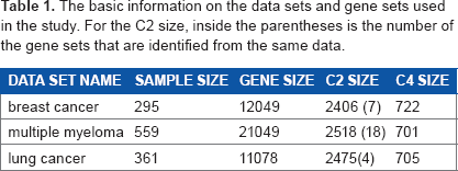
For each data set and each gene-set collection, we build 100 hybrid data models based on 100 different master genes following the approach defined in the Hybrid data model subsection. Because a master gene must be present in at least one gene set, due to the difference between the C2 and C4 collections, even for the same data set the hybrid data models built for the two collections are different. Moreover, in the C2 collection there are gene sets derived based on the same data sets used in this study. In our general simulation, we do not remove these gene sets from the study, but in the analysis, we evaluate the cases where all gene sets are included and the cases where these self-derived gene sets are removed. Table 1 provides a brief overview on the data sets and the associated gene sets.

Table 1

The basic information on the data sets and gene sets used in the study. For the C2 size, inside the parentheses is the number of the gene sets that are identified from the same data.

DATA SET NAME	SAMPLE SIZE	GENE SIZE	C2 SIZE	C4 SIZE
breast cancer	295	12049	2406 (7)	722
multiple myeloma	559	21049	2518 (18)	701
lung cancer	361	11078	2475(4)	705

For each hybrid model, we tested the GSA methods at three sample sizes: 20, 40, and 60. We specifically focused on the small sample cases since this is the area in which GSA methods are believed to be advantageous. For a given model and sample size, 100 data sets were sampled from the full data set to test reproducibility. Thus, altogether there would be 3 data sets, 2 gene-set collections, 100 data models, 3 sample sizes, 100 repeats, and 7 GSA methods, resulting in 1.26 million individual runs. All simulations have been implemented in R and conducted on a high-performance cluster computer system, with the full simulation taking more than 500,000 CPU hours.

Results and Discussion

As described in the simulation subsection, we used two genesets collections, C2 and C4, and analyzed the data by using all gene sets or by removing the self-derived gene sets. Due to limited space, in this section we focus on the results generated based on C2, with all gene sets used, and refer to other results only when necessary. Full results are available in the additional files.

Comparing the properties of selected hybrid data models

The 100 hybrid data models selected for each data set and gene-set collection evenly cover all possible prior distributions with minimum Bayes errors. This selection criterion does not provide information on other properties associated with the model. Hence, before examining the simulation results on various GSA methods, it is necessary to check the properties of the hybrid data models.

Figure 2 shows the property distributions of the selected models against the distribution of all models. Each plot is drawn in its own scale and should not be compared directly to other plots. It can be seen that the three data sets show considerable differences in most of these properties.

Figure 2.

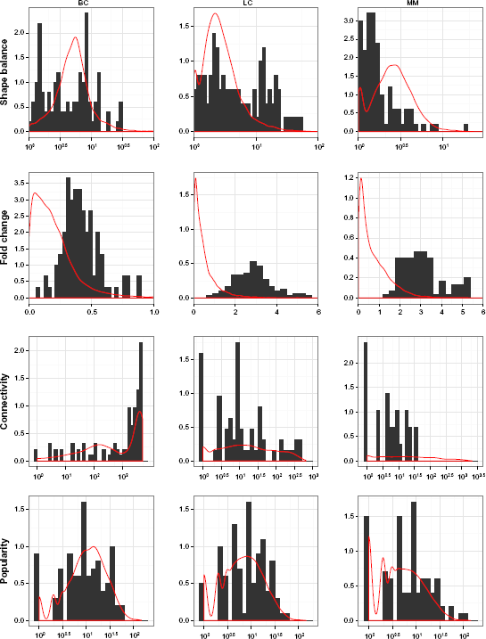
The general information on several important properties, including the shape balance, fold change, connectivity, and popularity, of the hybrid data models generated for gene set collection C2, for all three data sets. The histograms are the distributions of the 100 selected hybrid data models, and the red lines are the Gaussian density curves of all hybrid data models. Except fold change, all other properties are shown in log10 scale at x-axis. For connectivity, extra 1 had been added before the logarithm was taken. Note that each plot has its own scale.

For shape balance, the selected models all have somewhat different distributions than all models. BC and LC sets show that the selected models have evenly distributed shape balance in log scale, indicating there are considerable models possessing dramatically different variances in two classes, hence the extreme nonlinearity in the expression level distributions. As for MM set, although most models have rather unbalanced shape, most selected models have rather balanced shape.

For fold change, all three data sets show the selected models to be end-loaded at the large fold change region, which is not surprising since the models are selected partially based on the Bayes error, which is commonly believed to be negatively correlated with fold change. It is also reasonable to believe that master genes responsible for the phenotype variance should have significant fold change in expression levels to initiate qualitative change in the signaling pathways.

For connectivity, the selected models of all three data sets follow closely with other models. Only in the MM set are there no selected models with very high connectivity. In the BC set, a considerable number of models have very high connectivity. Since each model is associated with one gene, it shows that almost half of the genes have higher than 0.5 correlation to overall a thousand other genes, and some have connectivity as high as 5000. For the MM and LC sets, their general connectivities are quite low, smaller than 50 for the MM set and 500 for the LC set. The connectivity is quite evenly distributed in log scale. The high connectivity in the BC set indicates that there might be many genes and gene sets possessing similar expression pattern and association with the phenotype. Indeed, as shown in Venet D, Dumont JE, Detours V,³² by using the prognosis as phenotype labeling, 90% of random gene sets with more 100 genes will show a significant association with the prognosis. It has been shown in Nam D and Kim SY⁶ that if there are many gene sets containing differentially expressed genes that correlate with the phenotype, which is probably the case encountered in the BC set, then the Q1 based methods can provide more accurate P-values. And if there is only a handful of such gene sets, which might be the case in the LC and MM sets, then the Q2 based methods are more accurate in P-value prediction, as shown in Dinu I, et al.⁷ However, since in this study we are not concerned with the accuracy of P-values as in Nam D and Kim SY, Dinu I, et al,^6,7 the best ranking performance can come from any method, regardless of its accuracy in P-value estimation.

For popularity, again the selected models of all three data sets follow closely with other models. The distributions between the three sets are also quite similar. This is probably because the same gene set collection C2 is used, although the number of genes in the MM set is much larger than in the other data sets (see Table 1).

From the data set aspect, besides the tissue/disease difference, the two data sets using Affymetrix chips, MM and LC, show overall similar properties, compared to the BC set, which uses Agilent chips. It is hard to say how much of such difference is contributed by the microarray profiling technology. In any event, this difference indicates that the sample one might face in the real world can have quite different gene expression patterns and any observation collected from this study should only be applied to data of similar pattern, regardless of the technology or tissue type.

To further define the differences between the data sets, we examined the distribution of the Bayes error associated with each model for each data set. As described in the Method section, the models were selected to evenly cover the whole prior range [0.1, 0.5]. Since the Bayes error is not independent of the prior, but bounded by it, it is appropriate to compare the Bayes errors of a given model to the models with similar prior. In Figure 3, we show the scatter plot of Bayes error and prior of all three data sets. For more convenient comparison, the Bayes error is normalized with the prior. It can be seen that the BC data set has relatively high Bayes errors at all priors except in the range 0.15–0.2, indicating harder problems, while the MM and LC sets have lower errors. The example of ERBB2, which is based on the BC set and is shown in the Methods section, has a very low normalized error of 0.042.

Figure 3.

the scatter plot of normalized Bayes error with respect to prior. Gene sets: C2.

Figures 2 and 3 show that the selected models cover not only different priors, but also a wide range of other model properties. The models selected based on the gene-set collection C4 show overall a very similar pattern (see Additional File 2). For the details on exactly which genes are selected and the associated model properties, refer to Additional File 3.

Ability to reveal biological themes

We first evaluate the ability claimed by GSA methods to reveal potential biological themes. As described in the GSA methods subsection, we use the ranking of the true sets to compare GSA methods. A good GSA method should be able to rank the true sets at the top of the ranking list. Thus, for any ranking output a direct measure is whether any true sets are among the top k sets. Such a 0/1 score is not perfect, since only partial knowledge on true sets is available. For example, if both algorithms A and B cannot rank any true set at top k sets, our measure will give A and B an equal score. Yet if algorithm A ranks the gene sets closely related to true sets in the top k sets, while algorithm B ranks no closely related true sets in the top k, one would deem algorithm A to be relatively better than B; however, due to the lack of such information, such an advanced measure is not available in our study. Be that as it may, it is reasonable to believe that a good GSA method should be able to rank true sets higher than closely related sets and the just-described scenario only happens occasionally. Thus by conducting the experiments on more than 100 data models with 100 repetitions, the average performance, which is the percentage of cases that have true sets in the top k sets, should be able to deliver a meaningful performance evaluation.

Figure 4 compares the performance of different GSA methods at different sample sizes for each data set. The x-axis is the number of top sets selected and the y-axis is the corresponding percentage of cases containing the true sets.

Figure 4.

this graph compares GSA methods on ranking the true sets for different data sets and sample sizes. The x axis is the number of top gene sets, and the y axis is the percentage of cases that the true set is among the selected top gene sets. Gene sets: C2. All gene sets used.

Two Q2 methods, global test and SAMGS, split the best performance in all cases. The global test has the overall best performance. It has the best performance in the BC set. In the LC and MM sets, it ranks second best at sample sizes 20 and 40, while outperforming SAMGS for sample size 60, where the number of top sets picked is small, and almost indistinguishable when more sets are picked. Although SAMGS has excellent performance with the LC and MM sets, it has mediocre performance for the BC set at sample sizes 40 and 60. ANCOVA global test has similar yet poorer performance than global test in all data sets. For other methods, only GAGE has competitive performance in the LC set at sample size 20.

Clearly for the proposed data model, the Q2 methods, which determine the significance of the current gene set purely based on the gene set itself, provide much better ranking. In comparison, both the Q1 and Q3 methods compare the current gene set with the remaining genes, sometimes through extra permutation along genes. With the total number of genes over 10,000, such a computation might bring extra uncertainty, and probably contribute to the inferior performance. However, there could certainly be other factors, including the properties of the data sets used in this study, that affect the observed performance.

While the Q1 and Q3 methods demonstrate generally poor performance on all three data sets, the performance of the Q2 methods on different data sets is quite different. The BC set shows the greatest difficulty for all methods. Even the best performance can only be described as poor: at sample size 60, global test delivers true sets in slightly more than 40% of the cases for the top 5 sets and about 60% for the top 20 sets. In comparison, for both the LC and MM sets, and sample size 60, global test ranks the true sets in the top 5 sets more than 85% of the time and at or more than 90% in the top 20 sets.

We then evaluate the correlation between various model properties and the ranking performance to see if any properties can significantly affect the outcome. In summary, we found little significant or consistent correlation pattern between model property and ranking performance. However, the connectivity and median best rank show clear correlation for Q2 methods in the BC set. Thus, the connectivity could be a critical factor in the performance of GSA methods. The full results for all data sets and all properties, along with a more detailed discussion, are available in the Additional File 4.

Next, Figure 5 compares the performance of a given GSA method at different sample sizes. Among all methods, only global test and ANCOVA global test show consistent improvement with increase of sample size in all data sets. SAMGS has some improvement only from sample size 20 to 40, and from 40 to 60 the performance even decreases in the BC set. The two Q3 methods, GSA package and GSEA, show moderate improvement with sample size. The worst case is GAGE, which essentially shows no improvement at all, while the other Q1 method, SAFE, shows only slight improvement over sample size.

Figure 5.

this graph compares the performance of GSA methods on ranking the true sets for different data sets and GSA methods. The x axis is the number of top gene sets, and the y axis is the percentage of cases that the true set is among the selected top gene sets. Gene sets: C2. All gene sets used.

Table 2 shows a specific example based on ERBB2 with the BC set using the C2 collection. The performance on this model is generally very good for all methods. ANCOVA global test, global test, GSA package, and SAMGS have perfect or close to perfect performance from the smallest sample size. GSEA and SAFE improve their performance with larger sample size, while GAGE's performance drops slightly with increased sample size. The results are quite consistent with those in Figures 4 and 5, apart from GSA package's good performance. The full results for all models with the C2 collection with all gene sets and the C4 collection are available in Additional File 2.

Table 2

ranking performance of GSA methods on ERBB2 master gene of BC set, C2 collection. The median ranking of 100 repeats is shown here.

SAMPLE SIZE	ANCOVA	GAGE	GLOBAL TEST	GSA PACKAGE	GSEA	SAFE	SAMGS
20	3	10	1	2	10.5	15.5	1
40	1	11	1	1	1	14	1
60	1	13	1	1	1	6	1

The results shown in Figures 4 and 5 are based on all gene sets in the C2 category. If one removes the self-derived gene sets from all gene sets, then the general performance will decrease only slightly, as expected. The performances based on the C4 category share the general trends exemplified in the C2 category results, but can vary at some points. For instance, for C4 category, GAGE now has the best performance with the BC set at sample size 20, when more than 20 top sets are picked. The performance of GSA package decreases considerably in the MM and LC sets, but improves a bit for the BC set. The full results are available in Additional File 4.

Ability to ensure reproducibility

A common argument regarding GSA methods is that by using the gene sets instead of individual genes, the outcome is less susceptible to noise and therefore can lead to better reproducibility. Since the proposed model is built based on a relatively large data set, with the minimal sample size of 295, this allows us to generate multiple sample sets for each model from the same distribution and apply the GSA algorithm repeatedly to examine the reproducibility.

We first evaluate the reproducibility of the true set ranking performance. For each hybrid data model, the best ranks of the true sets for all 100 repeats are collected to obtain the standard deviation, and the histogram of all 100 data models are drawn. In Figure 6, the histograms of all seven GSA methods for the BC and LC sets at different sample sizes are shown, with the x-axis in log scale. (The results of the MM set, the models of which are based on a larger data set, are similar to the LC set. To save space, they are not shown here but are available in Additional File 5). For the model where the standard deviation is 0, we set the standard deviation to 10^-2, which is smaller than any possible case. This situation almost always indicates that all repeats rank a true set at the top position.

Figure 6.

Histogram of the standard deviation of the best rank. Gene sets: C2. All gene sets used.

The histograms indicate that in general, the GSA methods with better performance, ie, the Q2 methods, have relatively smaller variance in model repeats, and the variance decreases significantly with the increase of sample size. For other methods, not only the variance is large, but the improvement with sample size is limited. The global test has the smallest variance, and shows considerable improvement with sample size. For the LC set at sample size 60, 40% of the model's global test has zero variance. Although SAMGS's average performance is very good, many models have standard deviation around 10 and very few have zero variance. The variance of ANCOVA global test is very similar to global test in the BC set and slightly worse in the LC set.

The methods GSA package, GSEA and SAFE have highest variance, with GSA package the poorest. For most cases GSA package has standard deviation much larger than 100. Although the performance improves with sample size significantly, the standard deviation improves little with sample size, except for a handful of cases.

In general, there is a strong correlation between performance, measured by the median best rank, and standard deviation (results available in Additional File 5). For the cases where the percentage of true sets is low in the top ranked sets, the ranking of the true sets can often have a standard deviation, as high as 100. This indicates that for most GSA methods, the reproducibility is low, which further worsens the already poor performance.

The only exception is GAGE, which shows smaller variances despite its moderate performance among all GSA methods. To appreciate this phenomenon, we further examined the reproducibility of the ranking list among all repeats. For any two repeats of the same model, we compared the ranking lists of gene sets generated by two repeats and counted the number of gene sets that appear in the top 10 of both ranked lists. We conducted such pair-wise comparison in all repeats and took the average of the number of overlapped gene sets as the measure of reproducibility in the ranked list. For the 100 repeats used in our simulation, this means an average of more than 4450 pairs of repeats. We then constructed the histogram of this measure over all 100 data models. Figure 7 shows the histograms of all seven GSA methods for the BC and LC sets at different sample sizes (The results of the MM set are similar to the LC set. To save space, they are not shown here but are available in Additional File 5). In each histogram there is a red dot indicating the average of the number of overlapped gene sets for all repeats regardless of the data model. We have averaged all possible gene list pairs for 100 models x 100 repeats = 10,000 repeats. This dot reflects the global reproducibility of gene lists across the data models.

Figure 7.

Histogram of the average number of overlapping gene sets between repeats. Gene sets: C2. All gene sets used.

The reproducibility of GAGE is the highest among all GSA methods: on average there are 6 to 8 overlapped gene sets in any two repeats. The high reproducibility exists across the data models. In fact, there are gene sets appearing in more than 8,000 out of the 100,000 total repeats, no matter which data model is used. This phenomenon indicates that GAGE picks not the gene sets that most differentiate the response labels, but the gene sets showing most significant difference from other gene sets. The fact that GAGE's performance may have little relationship to the purpose of gene set ranking may explain its lack of improvement with increasing of sample size, as shown in Figure 5.

For other GSA methods, in general, the average number of overlaps is quite low when sample size is small, and the number increases when sample size increases. For three Q2 methods, at larger sample sizes, the distribution of average is widely spread and many models have more than 5 overlapped gene sets between repeats. For global test and ANCOVA global test, in some models for the LC set with sample size 60, almost all 10 top gene sets picked up in one repeat will appear in another repeat, indicating very good reproducibility. For GSA package, GSEA and SAFE, the number of duplicates increases at a much slower pace with sample size.

The average number of overlaps across the data models remains very low, close to zero in most cases, especially in the LC set. This is understandable because different data models represent different biological themes and should therefore lead to different gene sets in ranking. In the BC set, the global average in duplicates increases slightly with sample size. This is especially significant in SAMGS, where at sample size 60 there are on average 2 overlapped gene sets between any two repeats, regardless of the data model. A detailed examination shows that 16 gene sets appear in the top 10 gene set list of more than 1,000 repeats, with the most frequent 2 appearing in over 5,000 repeats. Further examination shows that these 16 gene sets happen to be among the first 17 gene sets provided in the gene set list file, indicating a strong bias associated with gene set list order. Since the P-value is computed through permutation, and we use 10,000 permutations for SAMGS in our simulation (see description in Additional File 1), this observation indicates the possibility that the resolution of the permutation test is not fine enough and there are many gene sets with the same low P-value (mostly zero), so that the gene sets positioned at the beginning of the list are more frequently selected.

To examine the possibility of such cases, we plot cumulative-distribution style plots in Figure 8 to check all GSA methods and data sets for all three sample sizes. In each plot, the x-axis denotes the gene sets ordered as in the gene list. The y-axis shows the total number of times that the gene sets up to that position have been selected in the top 10 of the ranked lists. SAMGS shows a strong bias associated with the order of gene sets, which is especially true in the BC set. In the LC and MM sets, the bias is not significant when sample size is 20 but becomes obvious at larger sample sizes. Such strong bias may explain why the performance of SAMGS decreases when sample size grows from 40 to 60 in BC set, as shown in Figure 5, and also why the variance of SAMGS does not decrease with sample size, as shown in Figure 6. It looks like the statistical test adopted by SAMGS is very sensitive, and many gene sets weakly associated with the response can exhibit strong P-values inseparable from true sets, which is a concern raised in the Background section.

Figure 8.

The effects of gene set list order. X axis denotes the gene sets ordered as given gene set file. Y axis shows the total number of times that the gene sets up to that position have been selected into the top 10 of the ranking lists. Gene sets: C2. All gene sets used.

All other methods except GAGE show a relatively diagonal line, which is almost unchanged for all sample sizes. This is as expected since for each model there are certain gene sets that should be more frequently selected into the top of the list, and by averaging over all data models the number being selected should be quite evenly spread over all gene sets. For GAGE, the plots show zig-zag curves. This is also unsurprising since GAGE's ranking list reflects the difference between gene sets, which varies little from model to model, as shown in Figure 7. Although the simulations have been conducted over 100 models, in all cases the same batch of gene sets is used. Thus, essentially GAGE has performed the ranking over the same gene-set population and the curve, although averaged over all models, is virtually a curve of one instance.

The results shown in Figures 6, 7, and 8 are based on all gene sets of the C2 category. However, there is little difference if one removes the self-derived gene sets from all gene sets. If the gene sets in the C4 category are used, again the general trends remain. In the C4 category, the bias associated with the gene set order for SAMGS is much weaker in the LC and MM sets, which is probably due to the much smaller gene set size. The full results are available in Additional File 5.

Impact of GSA method settings

One last issue to be pointed out is the impact of GSA method settings. As indicated in the GSA methods description, we noticed that GAGE provides two settings. We chose both directions to generate the main results for comparison. However, we found that by changing the gene-level statistics to same direction, the ranking performance of GAGE is significantly decreased, to the point of being among the poorest of in all methods. Furthermore, the high reproducibility between repeats as shown in both directions results in Figures 6, 7, and 8 also disappears. It is clear that the GSA method setting matters substantially in the ranking performance and the same settings can be either an advantage or disadvantage in different scenarios. However, since this is not the main focus of this study, interested readers are referred to Additional File 6 for a short discussion with full results for GAGE and ANCOVA global test.

Conclusion

We have conducted a comprehensive simulation study to compare seven popular GSA methods. From a practitioner's viewpoint, we examine the two widely accepted goals claimed by GSA methods: revealing biological themes and ensuring reproducibility for small-sample studies. We have focused on the ranking performance of the GSA methods, believing that a good GSA method should be able to consistently rank the true gene set at the top of the output. To be able to evaluate the performance in a more realistic scenario and to overcome the limitation on available real data sets, we have used a hybrid data model framework. Our data model assumes that there is a master gene whose expression profile directly determines the observed phenotype. The GSA methods are then applied to the data set generated by the hybrid data model to see if they can reveal the gene sets that contain a master gene. We also examine the ranking of such gene sets in repeats.

Our simulation shows that one must use GSA methods with caution since most GSA methods perform poorly on the proposed data model. They can hardly reveal true biological themes, nor can they ensure reproducibility between repeats. Based on our simulation, we would have the following recommendations for anyone who would like to use GSA methods to reveal biological themes with acceptable reproducibility:

•

Check your data. Data sets with high gene-gene connectivity can significantly compromise the performance of GSA methods.

•

Use Q2 methods. The global test provides the best average performance.

•

Examine the P-values. Methods with sensitive tests like SAMGS lose ranking ability quickly with the increase of sample size, which can be detected in the pattern of P-values. Switch to other methods if necessary.

•

Proceed with caution. Our simulation study assumes that the phenotype is determined by a single master gene's activity. Most biomedical interactions are much more complicated and the performance of GSA methods could be further compromised.

Owing to the design of the proposed model, we did not check the ability of current GSA methods to detect weakly differentiated genes and cases where the phenotypes are determined by the interaction of multiple master genes. However, we expect that such analyses will be even more challenging. For these, it may be wise to resort to more exact synthetic data models to understand the characteristics of GSA methods. Our future research will proceed in this direction.

Finally, some GSA methods extend the GSA analysis by reducing the significant gene sets to a few core genes that contribute most to the statistical significance, eg, leading edge analysis in GSEA package and significance analysis of microarray for gene-set reduction (SAM-GSR) for SAMGS. The accuracy of these gene set reduction approaches remains to be deeply examined.

Author Contributions

Conceived and designed the experiments: JH, MLB, ERD. Analyzed the data: JH. Wrote the first draft of the manuscript: JH, MLB, ERD. Agree with manuscript results and conclusions: JH, MLB, ERD. Jointly developed the structure and arguments for the paper: JH, MLB, ERD. Made critical revisions and approved final version: JH. All authors reviewed and approved of the final manuscript.

DISCLOSURES AND ETHICS

As a requirement of publication the authors have provided signed confirmation of their compliance with ethical and legal obligations including but not limited to compliance with ICMJE authorship and competing interests guidelines, that the article is neither under consideration for publication nor published elsewhere, of their compliance with legal and ethical guidelines concerning human and animal research participants (if applicable), and that permission has been obtained for reproduction of any copyrighted material. This article was subject to blind, independent, expert peer review. The reviewers reported no competing interests.

Supplementary Data

Additional file 1—pdf file

Detailed description on GSA methods and data sets used in this study.

Additional file 2—xlsx file

Detailed hybrid data model info.

Additional file 3—pdf file

Full results for the properties of selected hybrid data models.

Additional file 4—pdf file

Full results for the ability of GSA methods to reveal biological themes.

Additional file 5—pdf file

Full results for the ability of GSA methods to ensure reproducibility.

Additional file 6—pdf file

Full results and discussion on the impact of different GSA method settings.

Footnotes

Acknowledgements

The authors would like to thank Dr. Chao Sima for insightful discussion. The authors would also like to thank the High Performance Biocomputing Center at TGen for providing the computational support.

References

Subramanian

, Tamayo

, Mootha

V.K.

. Gene set enrichment analysis: a knowledge-based approach for interpreting genome-wide expression profiles Proc Natl Acad Sci USA. 2005; 102: 15545–50.

Efron

, Tibshirani

. On testing the significance of sets of genes. The Annals of Applied Statistics. 2007; 1: 107–129. Mathematical Reviews number (MathSciNet): MR2393843; Zentralblatt MATH identifier: 1129.62102.

Luo

, Friedman

M.S.

, Shedden

, Hankenson

K.D.

, Woolf

P.J.

. GAGE: generally applicable gene set enrichment for pathway analysis. BMC Bioinformatics. 2009; 10: 161.

Goeman

J.J.

, Bühlmann

. Analyzing gene expression data in terms of gene sets: methodological issues. Bioinformatics. 2007; 23: 980–7.

Liu

, Dinu

, Adewale

A.J.

, Potter

J.D.

, Yasui

. Comparative evaluation of geneset analysis methods. BMC Bioinformatics. 2007; 8: 431.

Nam

, Kim

S.Y.

. Gene-set approach for expression pattern analysis. Brief Bioinform. 2008; 9: 189–97.

Dinu

, Potter

J.D.

, Mueller

. Gene-set analysis and reduction. Brief Bioinform. 2009; 10: 24–34.

Glazko

G.V.

, Emmert-Streib

. Unite and conquer: univariate and multivariate approaches for finding differentially expressed gene sets. Bioinformatics. 2009; 25: 2348–54.

Ackermann

, Strimmer

. A general modular framework for gene set enrichment analysis. BMC Bioinformatics. 2009; 10: 47.

10.

Emmert-Streib

, Glazko

G.V.

. Pathway analysis of expression data: deciphering functional building blocks of complex diseases. PLoS Comput Biol. 2011; 7: e1002053.

11.

Hung

J.H.

, Yang

T.H.

, Hu

, Weng

, Delisi

. Gene set enrichment analysis: performance evaluation and usage guidelines. Brief Bioinform. 2011.

12.

Kim

S.Y.

, Volsky

D.J.

. PAGE: parametric analysis of gene set enrichment. BMC Bioinformatics. 2005; 6: 144.

13.

Abatangelo

, Maglietta

, Distaso

. Comparative study of gene set enrichment methods. BMC Bioinformatics. 2009; 10: 275.

14.

Yang

, Daigle

B.J.

, Petzold

L.R.

, Doyle

F.J.

. Core module biomarker identification with network exploration for breast cancer metastasis. BMC Bioinformatics. 2012; 13: 12.

15.

Scherf

, Ross

D.T.

, Waltham

. A gene expression database for the molecular pharmacology of cancer. Nat Genet. 2000; 24: 236–44.

16.

Olivier

, Eeles

, Hollstein

, Khan

M.A.

, Harris

C.C.

, Hainaut

. The IARC TP53 database: new online mutation analysis and recommendations to users. Hum Mutat. 2002; 19: 607–14.

17.

Bild

A.H.

, Yao

, Chang

J.T.

. Oncogenic pathway signatures in human cancers as a guide to targeted therapies. Nature. 2006; 439: 353–7.

18.

Tarca

A.L.

, Draghici

, Bhatti

, Romero

. Down-weighting overlapping genes improves gene set analysis. BMC Bioinformatics. 2012; 13: 136.

19.

Rocke

D.M.

, Durbin

. A model for measurement error for gene expression arrays. J Comput Biol. 2001; 8: 557–69.

20.

Lee

M.L.T.

. Analysis of microarray gene expression data. Boston: Kluwer Academic 2004.

21.

Carlborg

, Haley

C.S.

. Epistasis: too often neglected in complex trait studies? Nat Rev Genet. 2004; 5: 618–25.

22.

Fraley

, Raftery

A.E.

. MCLUST Version 3 for R: Normal Mixture Modeling and Model-Based Clustering Technical Report 504 Department of Statistics, University of WashingtonBox 354322, Seattle, WA 98195–4322 USA 2009.

23.

Bishop

C.M.

. Pattern recognition and machine learning. New York: Springer 2006.

24.

Vijver

M.J.

, He

Y.D.

, Veer

L.J.

. A gene-expression signature as a predictor of survival in breast cancer. N Engl J Med. 2002; 347: 1999–2009.

25.

Barry

W T.

, Nobel

A.B.

, Wright

F.A.

. Significance analysis of functional categories in gene expression studies: a structured permutation approach. Bioinformatics. 2005; 21: 1943–9.

26.

Barry

W.T.

. A statistical framework for testing functional categories in microarray data The Annals of Applied Statistics. 2008; 2: 286–315. Zentralblatt MATH identifier: 1137.62390; Mathematical Reviews number (MathSciNet): MR2415604.

27.

Goeman

J.J.

, Geer

S.A.

, Kort

, Houwelingen

H.C.

. A global test for groups of genes: testing association with a clinical outcome. Bioinformatics. 2004; 20: 93–9.

28.

Mansmann

, Meister

. Testing differential gene expression in functional groups. Goeman's global test versus an ANCOVA approach. Methods Inf Med. 2005; 44: 449–53.

29.

Shedden

, Taylor

J.M.G.

, Enkemann

S.A.

. Gene expression-based survival prediction in lung adenocarcinoma: a multi-site, blinded validation study. Nat Med. 2008; 14: 822–7.

30.

Zhan

, Huang

, Colla

. The molecular classification of multiple myeloma. Blood. 2006; 108: 2020–8.

31.