
Abstract
Since the 2001 envisioning of the Semantic Web (SW) (Scientific American
Introduction
The Web is inherently noisy and as such its extension is noisy as well. This noise is as a result of inevitable human error when creating the content, designing the tools that facilitate the data exchange, conceptualizing the ontologies that allow machines to understand the data content, mapping concepts from different ontologies, etc. For instance, noise can be a consequence of building Linked Open Data (LOD) from semi-structured or non-structured data. When LOD is built from non-structured data such as text using Named Entity Linking (NEL) or relation extraction tools – whose accuracy is not perfect – they generate erroneous triples. Thus, the integrity of the inference becomes questionable.
It is foolish to expect that the Web or the SW will ever be free of noise. Many research efforts concentrate on noise detection and data cleansing in the Web of data. Knowing that there will always be other instances or types of noise that will be overlooked, other research efforts focus on noise-tolerance instead. Most of the current work in the latter category targets adding some noise-tolerant reasoning capabilities without aiming for full semantic reasoning.
Humans are able to learn from very few examples while providing explanations for their decision making process. In contrast, deep learning techniques – even though robust to noise and very effective in generalizing across a number of fields including machine vision, natural language understanding, speech recognition etc. – require large amounts of data and are unable to provide explanations for their decisions. Attaining human-level robust reasoning requires combining sound symbolic reasoning with robust connectionist learning as outlined in [96]. “We argue that to face this challenge one first needs a framework in which inductive learning and logical reasoning can be both expressed and their different natures reconciled.” [5,96] However, connectionist learning uses low-level representations – such as embeddings – rather than “symbolic representations used in knowledge representation” [23,55]. This challenge constitutes what is referred to as the Neural-Symbolic gap. The aim of this research is to provide a stepping stone towards bridging the Neural-Symbolic gap specifically in the SW field and RDF Schema (RDFS) reasoning in particular.
This paper documents a novel approach that takes previous research efforts on noise-tolerance to the next level of full RDFS reasoning. The proposed approach utilizes the recent advances in deep learning – that showed robustness to noise in other machine learning applications such as computer vision and natural language understanding – for semantic reasoning. The first step towards bridging the Neural-Symbolic gap for RDFS reasoning is to represent Resource Description Framework (RDF) graphs in a format that can be fed to neural networks. The most intuitive representation to use is graph representation. However, RDF graphs differ from simple graphs as defined in the graph theory in a number of ways. We examine in the literature different graph models for RDF from which we conclude that the proposed models were neither designed for RDFS reasoning requirements nor are they suitable for neural network input. The proposed graph model for RDF consists of layering RDF graphs and encoding them in the form of 3D adjacency matrices. Each layer layout in the 3D adjacency matrices forms what we termed as a graph word. Every input graph and its corresponding inference are then represented as sequences of graph words. The RDFS inference becomes equivalent to the translation of graph words that is achieved through neural network translation.
The evaluation confirms that deep learning can in fact be used to learn RDFS rules from both synthetic as well as real-world SW data while showing noise-tolerance capabilities as opposed to rule-based reasoners.
Contributions and outline
The main contributions in this paper are:
In Section 2, we use three aspects to position our research with respect to the related work. Section 3 draws a taxonomy for noise types in SW data and illustrates the process of ground truthing and noise induction for LUBM and a subset of DBpedia – that are used as examples to describe the design of the overall approach. We examine different graph models for RDF and motivate the design of the layered graph model for RDF in Section 4. Then the creation of the RDF tensors and the RDF graph words as well as the description of the graph words translation are presented respectively in Section 5 and Section 6. The results of the experiments are described in the Section 7. In Section 8, we review the related literature in terms of noise-tolerance in the SW, deep learning and the SW and graph embedding techniques – specifically KG embedding. Finally the learned lessons, main contributions and future work are illustrated in Section 9.
Background and problem statement
In this section we use three aspects to position our research with respect to related work:
Noise handling strategies: active vs adaptive Knowledge graph completion categories: schema-guided vs data-driven Graph embedding output: Node/Edge embedding vs whole-graph embedding.
Noise handling strategies
We classify the strategies of handling noise in SW data into two categories:
Knowledge graph completion categories
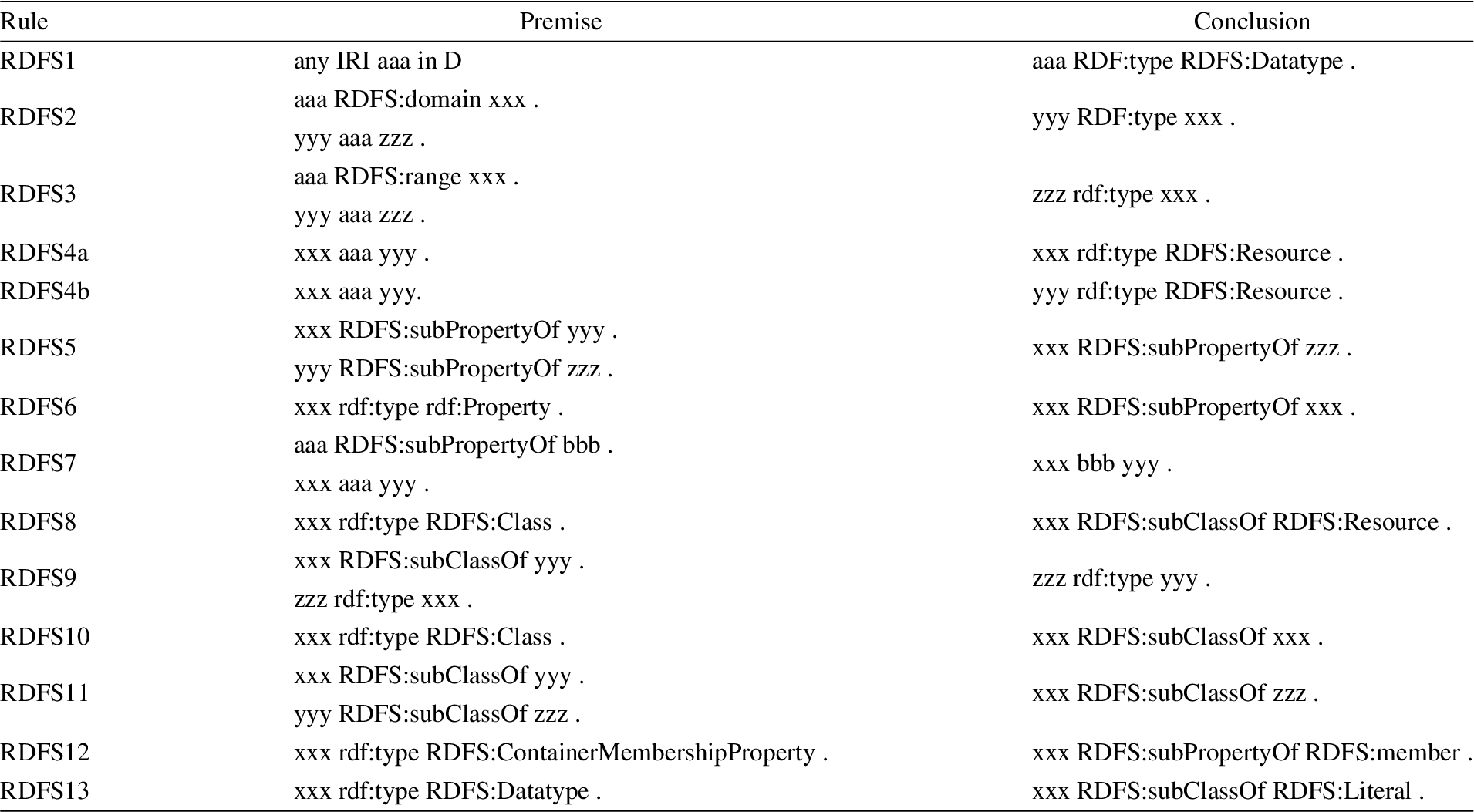
RDFS closure can be seen as a Knowledge Graph Completion (KGC) problem – multi-relational link prediction problem in particular – where each RDFS rule (see Appendix A) generates different types of links:
links between TBox concepts (RDFS10, RDFS11)
links between TBox properties (RDFS5, RDFS6)
links between ABox entities and TBox concepts (RDFS2, RDFS3, RDFS9)
links between ABox entities (RDFS7)
We refer to the RDFS closure computation as schema-guided KGC because the links are generated according to the ontology (TBox), unlike data-driven KGC where the links are predicted based on the analysis of the existing links in the KG. Data-driven KGC models “heavily rely on the connectivity of the existing KG and are best able to predict relationships between existing, well-connected entities” [5,88]. The predicted links from data-driven KGC might be seen as links between ABox entities and thus similar to the (d) case in the schema-guided KGC. However, there is a crucial difference: the generated relation (or link label) by the RDFS7 rule is a super-property that might not be seen in the initial KG as it is defined only in the TBox as a node not even as a link type, whereas all the relations generated by data-driven KGC are necessarily seen before in the initial KG.
Graph embedding output
Graph embedding approaches can be classified using several criteria. One particular criterion of interest in our survey of the state of the art (Section 8) is the “problem setting” [12]. The problem setting uses the type of graph input as well as the embedding output to classify the embedding approach. For the input part of the problem setting, the graph can be either:
The majority of graph embedding approaches (detailed in Section 8) yield node representation in a low dimensional space. This is why graph embedding and node embedding are often used interchangeably. However, there are other types of graph embedding outputs such as:
Problem statement
For learning RDFS reasoning, the whole-graph embedding is required because the input of the learning algorithm is the input graph and the output is the inference graph. However, existing embedding techniques for KGs were not designed for RDFS reasoning and they raise two main challenges if they were to be used for this task.
The first challenge is the need to check the validity of every possible triple using the scoring function The second challenge is the embedding of the relations that are seen only in the inference as the embeddings should be learned only from the input graph and be used to generate the inference graphs. For instance, when the property mastersDegreeFrom in LUBM appears in the input graph, its super-property degreeFrom appears in the inference graph by applying the RDFS7 rule [37]. If degreeFrom was not seen in the input graph then its embedding was not learned.
The baseline experiments detailed in Section 7.3 illustrate these challenges empirically.
Ground truthing and noise induction
For this research, the input is from one of two types of datasets: a synthetic dataset from LUBM and a real-world dataset from DBpedia [3]. The inferential target for these datasets is set using a rule-based SW reasoner (Jena [15]). Essentially, the goal for the deep reasoner is to learn the mapping between input RDF graphs and their entailed graphs in the presence of noise. Thus, noise was induced in the synthetic dataset to test the noise-tolerance of the deep reasoner.
Taxonomy of Semantic Web noise types

Semantic Web noise taxonomy.
The literature contains a few taxonomies [41,103] for the types of noise that can impact RDF graphs; however they are not drawn with respect to the impact of the noise on the inference. The taxonomy illustrated in Figure 1 serves this purpose. It should be noted that the propagation of noise is dependent on the inference rule.
TBox Noise is the type of noise that resides within the ontology, such as in the class hierarchy or domain and range properties. This type of noise impacts inference over the whole dataset. For example, in the DBpedia ontology, the property dbo:field has domain dbo:Artist which implies that every scientist in the DBpedia dataset who has a dbo:field property (such as dbr:Artificial_intelligence or dbr:Semantic_Web) will be labelled a dbo:Artist after inference. Reasoning with tolerance to TBox noise is outside the scope of this research for the following reason: the use of rule-based reasoners for ground truthing with noise in the TBox biases the whole ground truth, which makes noisy inferences omnipresent and not just anomalies that can be detected and fixed.
The following assumption is made in order to scope this research within a manageable framework:
The noise is latent only in the ABox, but the TBox is devoid of noise.
(Triple corruption).
The process of morphing an existing triple in an RDF graph by changing one of the triples’ resources. This can result in either propagable or non-propagable noise.
(Non-propagable noise).
Any corrupted triple in the input graph that does not have any impact on the inference.
This can occur at least in these cases:
The original triple does not generate any inference nor does the corrupted triple.
The original triple does not generate any triple but the corrupted triple generates an inference that is generated also by another triple in the input graph. (For example if the corrupted triple is equal to another triple in the graph)
The original triple and the corrupted triple generate the exact same inference.
The corrupted triple generates a set of triples that is a proper subset of the set of triples generated by the original triple. However the difference between the two sets is also generated by other input triples.
(Propagable noise).
Any corrupted triple in the input graph that changes the inference.
In order to discern the necessary conditions for RDFS rules to propagate noise, first the input patterns of the premises of the RDFS rules [37] are classified as TBox pattern or ABox patterns (Appendix B). The rules that have only TBox type patterns, such as RDFS5 (which defines the properties hierarchy) and RDFS11 (which defines the class hierarchy), are excluded because any corruption of triples matching these patterns will induce TBox noise. For the remaining rules that have both TBox and ABox patterns (i.e. RDFS2, RDFS3, RDFS7 and RDFS9), only the ABox triple can be corrupted. In Table 2, the necessary conditions for RDFS9 rule (Table 1) to generate a noisy inference from a corrupted triple are identified. In plain English, the RDFS9 rule will generate a noisy inference if and only if the corrupted type
RDFS9 rule from [37]

RDFS9 rule from [37]
Propagable noise by rule-based RDFS reasoners for RDFS9 rule

In [103], the authors examine different types of noise in the DBpedia instances. Thus all the categories of noise presented are of type ABox noise. Every category of noise can either be propagable or non-propagable depending on the property in the noisy triple. For example, in Object value is incorrectly extracted [103], the noise can be propagable if the corresponding property has any super-properties defined in the ontology and non-propagable otherwise – such as in the following example provided in the paper:

where the property dbpprop:map does not have any super-properties in the DBpedia ontology.
Ground-truthing in LUBM1
Lehigh University Benchmark (LUBM) [33] is a benchmark for SW repositories. The LUBM ontology conceptualizes 42 classes from the academic domain and 28 properties describing these classes’ relationships. LUBM1, an RDF graph of one hundred thousand triples, was generated according to this ontology, and contains
Noise induction in LUBM1
In [104], a methodology for noise induction in LUBM was proposed in which three datasets were constructed by corrupting type assertions according to a given noise level.
Instances of type TeachingAssistant were corrupted to be of type ResearchAssistant. This type of noise is non-propagable because both concepts, TeachingAssistant and ResearchAssistant, are sub-classes of the concept Person.
Instances of type GraduateStudent were corrupted to be of type University. This type of noise is propagable by the RDFS rule RDFS9 because these concepts are not siblings. A rule reasoner will generate a noisy inference by deducing that the student instance is of type Organization which is the super-class of University.
Instances of type Course were corrupted to be of type GraduateCourse. This type of noise is also non-propagable.
As [104] focus only on noisy type assertions, two additional datasets were created with noisy property assertions for the purpose of this research.
The property publicationAuthor is corrupted to be teachingAssistantOf. This noise is propagable by the RDFS rules RDFS2 and RDFS3 as the two properties have different domains and ranges. The property advisor is corrupted to be worksFor. This noise is non-propagable as the property worksFor does not have any domain or range specification in the LUBM ontology, but by removing the property advisor the type inference that was made about the student and advisor is lost.
Ground truthing the scientist dataset from DBpedia
From DBpedia [7], a dataset of scientists’ descriptions was built;
Number of resources per class in the scientists dataset
Number of resources per class in the scientists dataset
Despite its effectiveness as a standardized “framework for representing information in the Web” [22] and as an essential building block for the SW, the graph representation for the RDF model remains an open question in the SW research community. Even though the RDF conceptual model is designed as a graph, it differs from the graph theory definition of graphs in a number of ways. RDF graphs are heterogeneous multigraphs. Moreover, an edge in the ABox can be a node in the TBox (describing the properties hierarchy for example). Current research efforts to represent the RDF model as graphs – based on a: bipartite graph model [36], hypergraph model [55,63,100] or metagraph models [16] – target different goals ranging from storing and querying RDF graphs to reducing space and time complexity to solving the reification and provenance problem. Unfortunately, these goals do not coincide with RDFS reasoning. Moreover they use complex graph models which are not suitable for neural network input.
This paper describes a layered graph model that uses simple directed graphs to achieve the goal of representing RDF graphs and their inference graphs according to the RDFS rules. It is important to note that the mapping between RDF to the proposed layered model is irreversible – meaning that the reconstruction of the original RDF graph is not guaranteed. Thus, the layered graph model is not suitable for storing and querying RDF data.
Notations and definitions
In Appendix B, the premises of RDFS rules were classified into ABox patterns and TBox patterns.
TBox rule is a rule where its premises are all of type TBox pattern.
The Tbox rules in RDFS are:
RDFS5: the subPropertyOf transitivity rule RDFS6: the subPropertyOf reflexivity rule RDFS11: the subClassOf transitivity rule RDFS10: the subClassOf reflexivity rule
As these rules’ patterns are present in the ontological level and there is only one ontology per training set, there are not enough samples to learn these rules. Thus, it is assumed that there is a materialized version of the ontology where the TBox rules are already applied. This materialized version is inferred only once and is part of the training input. Let:
O: be the materialized ontology.
P: be the set of properties in O.
SubjObj(T): be the set of subject and object resources of the RDF graph T (formally defined in Appendix F).
A Layered directed graph is a graph that has multiple sets of directed edges where each layer has its own set of edges.
An n-layered directed graph is a layered directed graph of n layers. More formally, an n-layered directed graph is defined as:
Layered directed graph for RDF:
An RDF graph T is represented by a layered directed graph:
It is important to note that the transformation of an RDF graph into its layered directed graph representation is not bijective as two non-isomorphic RDF graphs can have the same layered directed graph representation.
Let T be an RDF graph and
However this transformation guarantees that if two RDF graphs have the same layered directed graph representation then their RDFS inference graphs according to the ontology O are isomorphic.
Appendix G lists two examples of layered RDF graphs: one for the graph description of the resource GraduateStudent9 and one for its corresponding inference graph.
The way the generic methodology of supervised machine learning is applied in this work is depicted in Fig. 2, where the pair (input, target) is the input graph and its corresponding inference. In a nutshell, tensors representing the input graph g and its corresponding inference i are created. The tensors of these graphs are then used in the training phase. The algorithm outputs the tensor of the graph and its encoding dictionary that will be used in the decoding phase to regenerate the original graph. In addition to preparing the RDF graph for input into a neural network, the main goal of this phase is to capture the pattern similarities between graphs in such a way that “similar” graphs will have similar tensors. An example of “similar” graphs is: two graphs containing RDF descriptions of two resources of the same type (such as two Publications’ descriptions in the LUBM1 dataset).

Encoding/decoding in training and inference phases.
The goal of this phase is to use the layered graph model for RDF in creating RDF tensors. Each RDF graph will be represented as a 3D adjacency matrix, where each layer is the adjacency matrix relative to one property (Figure 3). An ID must be assigned to each resource in the RDF graph to allow it to be represented as a 3D adjacency matrix. The process of assigning these IDs for the input graphs and their corresponding inference graphs must satisfy the following requirement:

3D adjacency matrix.
The proof for this requirement is detailed in Appendix H.
In the simplified version of the algorithm, two dictionaries were created: one for the subject and object IDs – which is split into a global and a local dictionary – and one for the property IDs. The global resources dictionary contains the subject and object resources that are used throughout the G set (which are basically the RDFS classes in the ontology). The local_resources_dictionary is created incrementally during the encoding routine for each graph g in G. It holds the IDs of the resources that are not present in the global_resources_dictionary. The local_resources_dictionary is populated with an offset equal to the length of global_resources_dictionary – that is, 57 in the case of LUBM1. The largest ID in the local_resources_dictionary for every graph in G is less than 80. This value is used to initialize the size of the 3D adjacency matrix. These dictionaries are then used in the encoding routine to transform a layered graph representation into an RDF tensor and vice-versa in the decoding routine. The details of the encoding/decoding algorithms are in Appendix I.
The previously stated goal – capturing the pattern similarities between graphs describing resources of the same type – can be achieved by this simplified encoding technique when the cardinality of each property is variable within a small range. For instance, in LUBM1, students take more or less the same number of courses, and a publication has between one to seven authors. To get the full list of these statistics, the following SPARQL query is run:

The inner query counts the number of objects per property per class and the outer query concatenates the possible values. Appendix M contains a sample of these statistics in LUBM1.
Alas, this is not the case in real-world knowledge graphs such as DBpedia, where even graphs describing resources of the same type differ widely. For example the DBpedia graph describing Professor James Hendler [24] has 40 objects for the property RDFt including owl:Thing, foaf:Person, dbo:Person, dul:Agent, dbo:Agent, dbo:Scientist, schema:Person, yago:Scholar110557854, etc. Out of these 40 objects, 12 are in the global_resources_dictionary because they are concepts in the DBpedia ontology and the other 28 objects will populate the local_resources_dictionary. In contrast, the DBpedia graph describing Professor Yoshua Bengio [25] has only 12 links for the property RDFt and all of the objects are in global_resources_dictionary. This implies that the RDFt layers in the 3D adjacency matrices for Professor Hendler and Yoshua Bengio graphs will be very different. In fact all the subsequent layers will be very different. For instance, when encoding the layer of the property dbo:almaMater for Professor Hendler’s graph, the resources dbr:Brown_University, dbr:Southern_Methodist_University and dbr:Yale_University will have IDs 29, 30 and 31 respectively as there is already 28 resources in the local_resources_dictionary. When encoding the same layer for Professor Bengio’s graph, the resource dbr:McGill_University will have ID 1 as the corresponding local_resources_dictionary is still empty. Consequently, this has a domino effect on the rest of the layers. To overcome this limitation, a more advanced tensor creation method was necessary to capture the patterns of real-world knowledge graphs.
Advanced version
The main idea of the advanced encoding/decoding technique is to create a local_resources_dictionary per layer instead of a local_resources_dictionary for the whole graph being encoded. While this may seem sufficient to overcome the limitation of the simple encoding technique, a few challenges in the encoding of the inference graphs as well as in the decoding phase for both the input and the inference graphs are encountered. The details of these challenges and the proposed solutions for the advanced tensor creation technique are detailed in Appendix J. When using the advanced encoding technique, the number of properties is actually the number of “active” properties – where active properties are the set of properties in the T-Box that are used in the A-Box. This reduces the size of the 3D adjacency matrices dramatically especially in the case of the Scientists dataset where only a small subset of the DBpedia properties are used.
Graph words
At this stage, every RDF graph is represented as a 3D adjacency matrix of size: (number_of_properties, max_number_of_resources, max_number_of_resources) where each layer represents an adjacency matrix according to one property.
In theory the maximum number of possible layer layouts in a dataset of size dataset_size is:
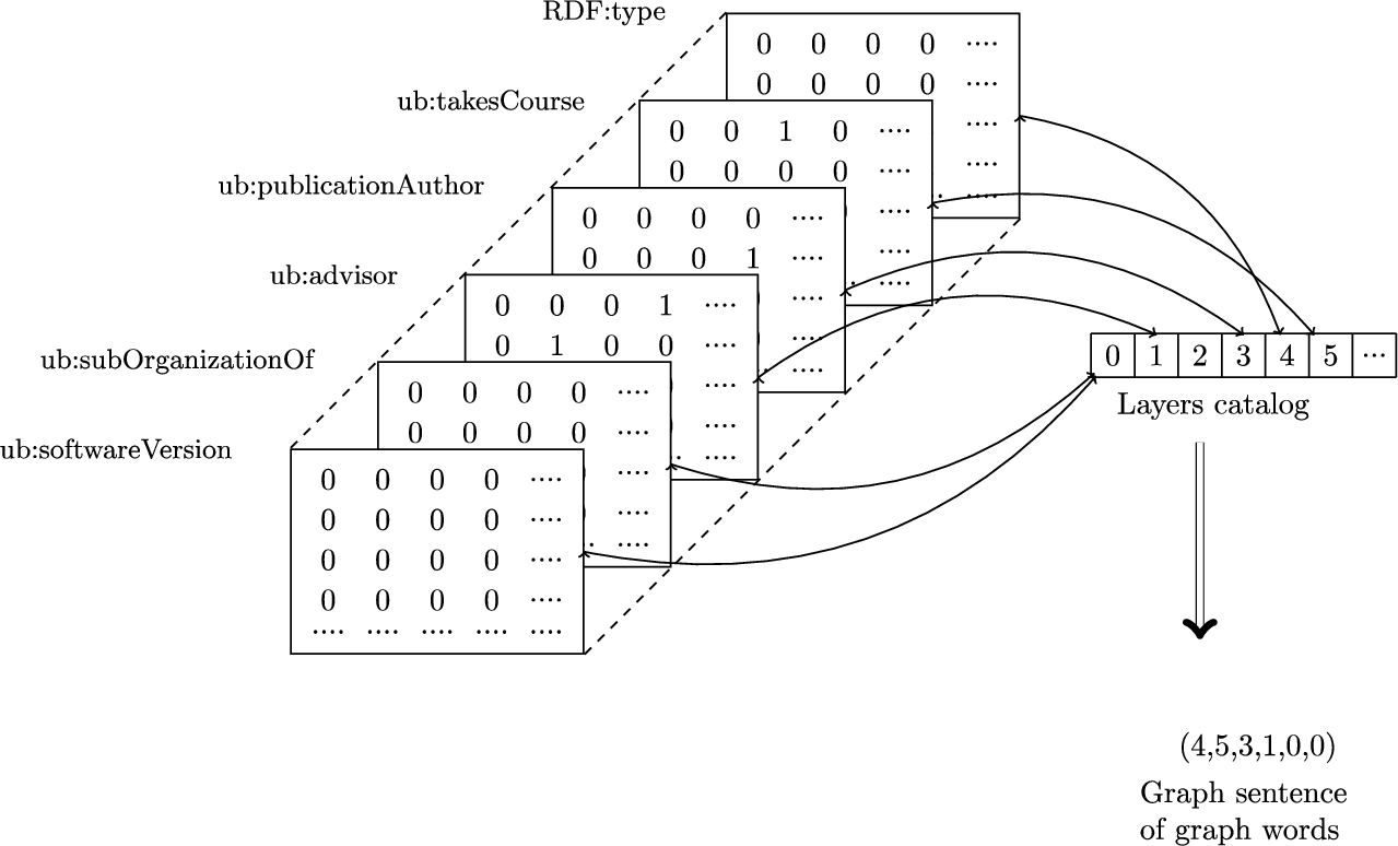
From a 3D adjacency matrix to a sentence of graph words.
Reducing the size of the encoded dataset: only the ID of the layer’s layout along with a catalog of layouts is saved.
Exploitation of the research results in neural machine translation.
At this stage, there is a parallel corpus of graph words for the input and inference graphs. This representation has the following drawbacks: difficulty handling “unknown” graph words and insensitivity to graph word similarities. Unknown graph words can be encountered when a graph word is seen only in the test set but not during the training phase; when inducing noise, most of the graph words will be unknown. A common technique in Natural Language Processing (NLP) is to assign the same ID for unknown words, which is not a significant deterrent to success in most learning tasks involving natural language. However, in our case if the same ID is assigned to every unknown graph word, then the learning process will be compromised and will not generate the exact inference. (Briefly, the proof by construction – that the use of the same ID for every unknown graph word is deterrent to learning the graph words translation – consists of building two graphs having the same input representations but having different targets.)

Graph words translation model for LUBM1.
By encoding an RDF graph as a sequence of layers where each layer contains an adjacency matrix of a directed graph according to one property, homogeneous graph embedding algorithms can be used on each layer. The High-Order Proximity preserved Embedding (HOPE) algorithm [70] was used as it had the best reconstruction accuracy when tested on the catalog of graph words. The graph words embedding also solves the problem of capturing the similarities between graph words.
By representing the RDF graph input as well as its corresponding inference graph by two sequences of graph words, the RDFS inference becomes equivalent to the translation of graph words. Thus, Neural Machine Translation (NMT) models can be applied to learn the RDFS inference generation. NMT models typical architecture consisted of [17] Recurrent Neural Network (RNN) Encoder-Decoder where the encoder RNN transforms the sequence of words from the input sentence into a fixed-length hidden representation and the decoder RNN generates the target sentence from the hidden representation. More recent architectures that used convolutional networks for NMT such as [29] outperformed RNN based architectures in terms of accuracy and training speed.
For designing the graph words translation model, we used keras [18] with TensorFlow [1] backend. It is basically a sequence-to-sequence model [93] with a Bidirectional Recurrent Neural Network (BRNN) [85] encoder. The overall architecture of the model is depicted in Figure 5. The input layer consists of a tensor of shape
For the training phase, we used Adam [48] optimizer – with a learning rate of 0.001, a first moment decay rate of 0.9 and a second moment decay rate of 0.999 – and a categorical cross-entropy for the loss.
Hardware setup
The training was done on a server, which has four Tesla K40m NVIDIA Graphics Processing Unit (GPU)s. Each GPU has 2880 Compute Unified Device Architecture (CUDA) cores and 12 GB of memory. The models were trained using all the GPUs in parallel.
Data analysis
In this section, we perform a statistical analysis on the training data for both LUBM1 and the scientists’ dataset. This analysis is based on the relations’ distribution across the training input and inference graphs. The motive behind this analysis is to get an insight to the performance of type prediction approaches on these datasets in comparison with our proposed approach.
LUBM1 data analysis
When we consider all the triples in the inference of LUBM1 across all the graphs, there are

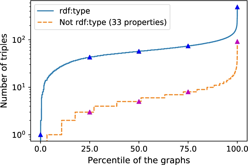
The distribution of properties in LUBM1 inference.

Frequency of the properties in LUBM1 inference.
Given these statistics about the frequency of properties in LUBM1 inference, it can be concluded that the upper bound of accuracy for type prediction systems is around

Distribution of properties in input and inference graphs in LUBM.
The Scientist’s dataset contains more than fifty thousands graphs. When considering all triples in the inference of these graphs, there are
Baseline experiments
As discussed previously in 2.4, existing KG embedding techniques that were designed for data-driven Knowledge Graph Completion (KGC) are not suitable for RDFS reasoning for the following reasons:
For learning RDFS reasoning, the whole-graph embedding is required rather than node/edge embeddings. The closure computation requires checking the validity of every possible triple using the scoring function. More importantly, any relation that is seen only in the inference (for instance generated by the RDFS7 rule [37]) cannot be learned from the input graph.
On the other hand, these techniques are more suitable to learn from the whole KG at once and there is no need to partition the KG into subgraphs containing resource descriptions as in our approach.
In order to set the baseline and provide empirical evidence of the previous claims about using KG embedding techniques for RDFS reasoning, we run the following experiments: the embedding of LUBM1(
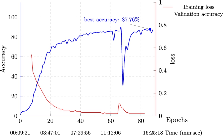
Evaluation on intact LUBM1
Figure 11 shows the training process on the LUBM1 dataset. After approximately 12 minutes of training,
Frequency of the properties in the scientists dataset inference.

RDFS inference with KG embedding techniques?
Table 4 presents the overall per-triple precision and recall as well as the breakdown of these metrics for each property in the inference. The precision and recall are much higher for the properties rdf:type and ub:degreeFrom compared with ub:memberOf. This can be explained by the fact that the property ub:memberOf is much less frequent in the LUBM1 training set of – which contains only one university.
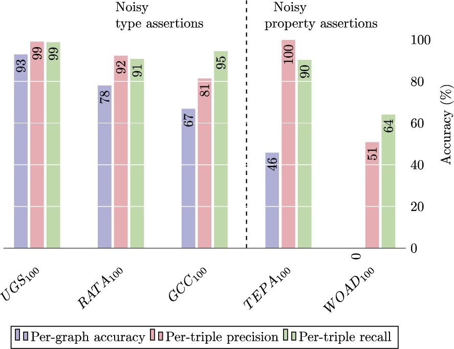
In this experiment, the trained model was tested on the noisy datasets created as described in Section 3. Two metrics were designed:
Jena materialization from the intact graphs (J) The deep reasoner materialization from the corrupted graphs ( An OWL-RL [64] materialization of LUBM1 to check the validity of the false positives from the deep reasoner. It is counter-intuitive that our approach performs better on propagable noise such as UGS compared with non-propagable noise such as GCC. This can be explained by the fact that the propagable noise case is very unlikely and there are no “similar” graphs in the training set. For instance, in UGS a ub:GraduateStudent is corrupted to be of type University, which makes the university take a course in the input graph. Being more “similar” to students’ graphs, it is inferred to be of type ub:Person rather than ub:Organizartion. This is not the case for non-propagable noise such as GCC where a ub:Course is corrupted to be of type ub:GraduateCourse, which is likely – i.e. “similar” graphs can exist in the training set.
Let V be the set of valid false positive triples. The quasi-confusion metric is computed as shown in Figure 14. The macro and micro evaluation on the 5 noisy datasets (Fig. 12) shows exceptional noise-tolerance compared to rule-based reasoners: 99% for the deep reasoner vs 0% (by design) for Jena in the
Evaluation on the scientists dataset
The model used for the scientists dataset is like the LUBM1 model, except for the hyper-parameters. Training to a validation accuracy of
(the first should be missed), and generated the following extra triple:

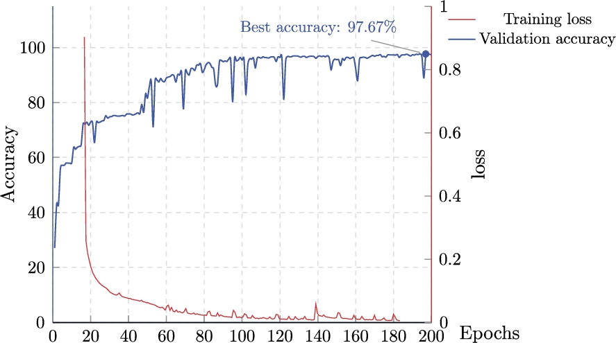
Training results on intact LUBM1 data.
Per-property precision and recall on LUBM1 test set
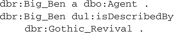
It should be noted that this information is not explicitly (i.e. embedded in the DBpedia graph of the resource dbr:Big_Ben) nor implicitly (i.e. can be inferred). It is therefore counted as false positive even though it “makes sense”. The deep reasoner inferred this information by capturing the generalization that resources with similar links to dbr:Big_Ben are usually of type dbo:HistoricPlace.
Macro and micro evaluation on noisy LUBM1 datasets.

Macroscopic metric: per-graph accuracy.

Refined confusion matrix.
Training results on DBPpedia scientists dataset.
In this section we review the state of the art in terms of:
Handling noise in SW data Graph embedding (KG embedding in particular) Approximate semantic reasoning Deep learning for semantic reasoning
Handling noise in Semantic Web data
The strategies for handling noise in SW data can either be active or adaptive:
Active noise handling
Most of the work in this category focuses on detecting and fixing noisy data in the LOD. LOD can be created using structured, semi-structured or non structured data. DBpedia [3], for example, is created from semi-structured Wikipedia articles. Non structured texts can also feed NEL tools to create LOD. These two methodologies are more likely to generate noisy triples due to the non perfect accuracy of NEL tools.
In [75], the authors describe two algorithms that they designed to improve the quality of LOD. The SDType algorithm falls into the category of adaptive noise handling and will be described in the corresponding section. SDValidate identifies wrong triples when there is a large deviation between the resource types. The main idea of this algorithm is to assign a relative predicate frequency – describing the frequency of predicate/object combinations – for every statement. Probability distributions are then used to decide if a statement with low relative predicate frequency should be considered erroneous. Both algorithms are validated on DBpedia and Never-Ending Language Learning (NELL) [14] knowledge bases.
In [104], the authors focus on detecting noisy type assertions. They built a few synthetic noisy datasets based on LUBM. Then a multi-class classifier is trained to learn disjoint classes.
In [27 ,99], the focus is on incorrect numerical data in LOD datasets. [27] uses a two phase detection approach. In the first phase, outliers of numerical values are detected for every property and in the second phase, the owl:sameAs property is used to confirm or reject the outliers. [99] uses a few unsupervised learning techniques including Kernel Density Estimation (KDE) [73] combined with semantic grouping to identify the outliers.
Adaptive noise handling
Given the unrealistic expectation of cleansing every type of noise in SW data, adaptive noise handling approaches focus rather on building techniques that are noise-tolerant. In the SDType algorithm [74,75], the rdf:type inference uses information from the ABox rather than ontological descriptions from the TBox. For instance, instead of using the rdfs:domain and rdfs:range of the properties to infer the resources’ types, which will propagate noise, a weighted voting heuristic is used instead to determine the types of the resources. The weights are generated from the statistical distribution between predicates and types. For example, given that the property dbo:location is mostly connected to objects of type dbo:Place, then this property will have high weight to infer the type dbo:Place.
To the best of our knowledge, most of the previous work in the literature about reasoning with noisy SW data focuses on type inference. This research is the first to aim at full RDFS reasoning with noise-tolerance capability.
Graph embedding
This review is partially based on three recent surveys of graph embedding techniques and their applications [12,31,97]. We update the latter survey by including the work on RDF graph embedding. The authors of [31] also provide an open source Python library (Graph Embedding Methods) for graph embedding comparison that we used to compare the discussed embedding techniques on RDF graphs.
It is needless to stress the omnipresence of graph based representations for research problems and real world applications ranging from social network analysis to recommendation systems to protein interaction networks to knowledge graphs and SW graphs in particular. This can be considered as the main motive for graph analytics research. Graph analytics tasks include centrality analysis, nodes classification [6], link prediction [52] etc. The latter is the closest to our research because the inference RDF graph can be seen as the link prediction applied to the input graph.
Why embedding graphs?
In performing the previous tasks of graph analytics, two of the main challenges – especially when processing large scale graphs – are size and time complexity. One technique that tackles these challenges is graph embedding. In a nutshell, the embedding consists of finding a mapping from the original space to a continuous vector space of lower dimension while preserving certain required properties. In graph embedding, the desired properties to be preserved can be node proximity, node similarities or dissimilarities, structural proximity etc.
How to embed graphs?
In order to briefly describe the embedding process, a few preliminary notions from [31] should be introduced. Let:
S be the adjacency matrix of the graph The first-order proximity between two nodes is defined as the weight of their edge. The second-order proximity between two nodes is defined by the similarity between their respective immediate neighbors. More formally, let Given a graph
Similarly, higher order proximity can be defined using the second-order proximity. Using these preliminary notions, [31] defines graph embedding as:
Graph embedding methods
Based on the techniques used to compute such embeddings, a taxonomy for graph embedding approaches can be drawn:
Matrix factorization methods Matrix factorization consists of decomposing a matrix into two or more matrices where their product regenerates the original matrix. Graph embedding techniques using matrix factorization start by generating a matrix representation of the graph and then compute the factorization to obtain the embedding. In its simplest form, the matrix representation of the graph can just be the nodes’ adjacency matrix S. Other matrix representations of the graph include the Laplacian matrix [4] and the Katz similarity matrix [46], which measure the nodes’ centrality. A few examples of graph embedding approaches using matrix factorization are: Locally Linear Embedding [81], Graph factorization [2] and HOPE [71]. The authors of the HOPE algorithm aimed to preserve the asymmetric transitivity property, which is an important property in directed graphs. The feature of preserving the asymmetric transitivity is desirable in RDF graphs embedding as the rdfs:subPropertyOf and rdfs:subClassOf are asymmetric transitive properties. In order to speedup the matrix factorization of sparse matrices, the authors of HOPE use singular-value decomposition.
Random walks methods [58] defines random walks on graphs by: Given a graph and a starting point, we select a neighbor of it at random, and move to this neighbor; then we select a neighbor of this point at random, and move to it etc. The (random) sequence of points selected this way is a random walk on the graph. [5,58]
Graph neural network models One of the earliest work that proposes a framework for consuming graph data by neural networks is GNN [83]. Deep autoencoders can be used for dimensionality reduction. Deep graph embedding techniques use this ability to reduce the dimension of the matrix representing the graph. The authors of [49] propose a Graph Convolutional Network (GCN) model which is a variant of convolutional neural networks that operates on graphs. [50] applies variational autoencoders – where the encoder part is a graph convolutional network – in order to improve the embedding quality of unsupervised techniques.
Embedding of knowledge graphs
[97] classifies the embedding approaches of KG facts into:
Let:
be the embedding space where d is the embedding dimension. be the vector representation in be the vector representation in
Neural network architectures for KG embedding The network models proposed in the literature for learning KG embeddings include:
Semantic matching energy [8] which computes the energy by matching the embedding of a left hand side containing the head and the relation of the triple and the embedding of the right hand side containing the tail and the relation of the triple.
Neural tensor network (NTN) [90] proposed an end-to-end deep neural network model that is parameterized by a 3-way tensor representing the relation in order to learn the plausibility of triples in a KG.
Relational Graph Convolutional Networks (R-GCNs) [84] adapts GCN [49] to KGs by introducing transformations that are dependent on the type and direction of the edges.
Embedding of RDF graphs RDF embedding techniques can be classified into:
Knowledge graph completion One of the main application of KG embedding is Knowledge Graph Completion (KGC). Data-driven KGC literature includes [45,54,80,86,91,94]. Logic Tensor Networks [86] allow the definition of logical constraints to improve the KGC. [80] aims not only at predicting missing relations in a KG but also at inducing the logical rules from it.
Approximate semantic reasoning
In 2010, Hitzler and van Harmelen called in [39] for questioning the model-theoretic semantic reasoning and investigation of machine learning (ML) for semantic reasoning since ML techniques are more tolerant to noisy data.
Type inference
Type inference consists of inferring the corresponding classes from the TBox for resources in the ABox. It can be considered as a main step towards full RDFS reasoning as almost half of the rules in RDFS – namely RDFS1, RDFS2, RDFS3, RDFS4a, RDFS4b and RDFS9 [37] – generate type inference.
SDType algorithm [74,75] (mentioned previously) used a statistical distribution of types to predict the type of object and subject in a triple given that they are connected with a certain property. Their statistical approach makes this type inference mechanism robust to noise in RDF data. [68] targeted inferring the missing types in DBpedia resources through an inductive and an abductive approach. In the inductive approach, the k-Nearest Neighbors algorithm is used to determine the closest concepts from the DBpedia ontology to which the resource should be linked. In the abductive approach, the Encyclopedia Knowledge Paths [67] are used in a similarity metric.
Consistency checking
In [76], the authors aimed to detect systematic errors in DBpedia by aligning the DBpedia ontology and the upper level ontology DOLCE-Zero [28]. By clustering the reasoning results, they found that 40 clusters cover 96% of the inconsistencies. This observation was among the motivations that approximate semantic reasoning can cover most of the use cases where ontological reasoning is required. In order to speedup the process of ABox consistency checking, [77] used an approximate semantic reasoning approach based on machine learning. The authors formalized the problem as a binary classification problem where each classifier C is trained for a specific TBox to decide if any ABox is consistent or not with respect to the TBox. In order to transform the RDF graphs into feature vectors, graph walks [57] were used. The decision tree model achieves 95% accuracy within 2% of the time required by a semantic reasoner.
In [60], the authors extend the clash queries [51] for DL-Lite [13] and caching to reduce the required calls to a semantic reasoner in order to check ABox inconsistency. This approach had better running time and empirical accuracy than [77].
Deep learning for semantic reasoning
One of the closest research efforts to the scope of this research is [42]. Besides the used neural network model, the main difference between their approach and ours is that they consider only learning from intact data and do not focus on noise-tolerance capabilities. In this work, Relational Tensor Networks (RTN) are proposed as an adaptation of Recursive Neural Tensor Networks (RNTN) [92] for relational learning. RNTNs were originally designed by Socher to support learning from tree-structured data such as sentences’ parse trees and they were used successfully to improve sentiment analysis results. In [42], the authors start by building a Directed Acyclic Graph (DAG) representation of the RDF input. Every resource in the graph is initially represented as an incidence vector that indicates the set of rdf:type(s) of the resource. Then the embeddings of the resources are computed using the RTN model that takes into consideration the type or the relation that each resource has. Two types of targets are considered: a unary target for type prediction and a binary target for predicate classification. The input for the binary targets are the embeddings of two resources – to which the predicates are being classified.
Conclusions, discussions and future work
The main contribution of this paper is the empirical evidence that deep learning (neural networks translation in particular) can in fact be used to learn semantic reasoning – RDFS rules specifically. The goal was not to reinvent the wheel and design a Yet another Semantic Reasoner (YaSR) using a new technology; it was rather to fill a gap that existing rule-based semantic reasoners could not satisfy, which is noise-tolerance.
While the current approach proves empirically that RDFS rules are learnable by sequence-to-sequence models with noise-tolerant reasoning capabilities, it is barely a scratch on the surface of noise-tolerant reasoning in general. This research can be extended in the following directions:
Generative adversarial model for graph words
The experiments on controlled noisy datasets from LUBM1 showed that the noise-tolerance capability of the deep reasoner depends on the type of noise – specifically the noise-tolerance on noisy type assertions is better than the noise-tolerance on noisy property assertions. In the propagable noise cases – where Jena or any rule-based reasoner generates noisy inferences – the deep reasoner showed noise-tolerance with varying degrees of accuracy (from
OWL reasoning
In this work, we tackled the problem of noise-tolerant RDFS reasoning. Web Ontology Language (OWL) reasoning with noise-tolerant capability is also a very promising research track that can find its applications in the biological and biomedical fields for example. We investigated some use cases using ontologies from the Open Biological and Biomedical Ontology (OBO) Foundry [89], specifically using the Human Disease Ontology [47]. In this use case, some patients’ descriptions would contain misdiagnoses and the goal is to generate correct inferences with the presence of these misdiagnoses. The hurdle that we faced in proceeding with this use case was ground truthing, as we needed patients’ data with tagged noise. In this context, tagged noise means that the misdiagnosed cases are known. This is required to compare the inference from intact data versus the inference from noisy data.
In [59], we tested the naive sequence-to-sequence learning approach on a subset of OWL-RL rules. This subset includes what we call generative rules that generate inference triples and exclude the consistency checking rules. The performance of the naive sequence-to-sequence approach on OWL-RL rules was comparable to its performance on RDFS rules. This is a preliminary indication that the graph words translation approach can also be applicable to learning OWL-RL rules.
Training with multiple “ABoxes”
Another limitation to the current approach is that the training is done on a dataset that uses only one ontology for the inference. After training the graph-to-graph model on the LUBM1 dataset, we needed to adapt the model hyperparameters for the scientists’ dataset and start the training from scratch. We propose exploring transfer learning: Instead of starting the training process from scratch when training to infer using a new ontology, the neural network weights from the previous training can be used to initialize the new model. Transfer learning [72] aims to capitalize on the knowledge learned from one domain and adapt it to a new domain. The adaptation phase in neural networks consists of tuning the model weights after initializing them using the previous models’ weights. Research in this direction looks promising especially when transferring weights between models of different width. The width of the model is determined by the length of the graph words sequence.
Towards the trust layer
In a recent positional paper titled “Semantic Web: Learning from Machine Learning” [11], Brickley describes his vision of how deep learning and SW fields can communicate and learn from each other. In this paper, we initiated the communication in one direction which is: deep learning for SW. The other direction, SW for deep learning, is also equally important and very promising with lots of opportunities for research and subsequent discovery. One such research effort in that direction is [82] where the authors use SW technologies to describe the inputs and outputs of neural networks.
We believe that our deep learning for noise-tolerant semantic reasoning contribution can be extended into a hub where both fields can communicate and benefit from each other. One way to create this hub is through provenance-based reasoning. Imagine that the deep reasoner will not only have access to the erroneous triple in DBpedia but to the provenance of that triple i.e. the person who originally edited the Wikipedia page and input the wrong information. By detecting that most of the triples provenant from that user causes the reasoner to be in noise-tolerance mode, it should not only ignore the triples generated by that user but also assign a trust level to its “facts”. This can be a step towards the trust layer in the SW layers cake.
Footnotes
Acknowledgements
We would like to thank DARPA SMISC, AFRL NS-CTA and IBM HEALS for sponsoring different stages of this research.
RDFS rules
RDFS rules (from [37])
Pattern types of RDFS rules’ premises
Pattern types of RDFS rules’ premises

Propagable noise by rule-based RDFS reasoners
Propagable noise by rule-based RDFS reasoners

Input graph g
Inference graph of the input graph in Listing 1
RDF graph formalism
An RDF graph can be defined using these formalisms from [34,40,63] (that is updated in this paper to conform to the more recent RDF 1.1 recommendation [22]:
Let:
A tuple
An RDF graph is a set of RDF triples.
Let:
Layered graph examples
Let the tuple of properties in
Proof of the tensor creation requirement
Tensor creation detailed algorithms
In order to fulfill the requirement established in Proposition 1, it is mandatory that the global_resources_dictionary and the local_resources_dictionary for a given graph g contain all the possible resources that might be used in its corresponding inference graph i. To create the properties dictionary Properties_dictionary, the list of properties is collected using the following SPARQL Protocol and RDF Query Language (SPARQL) query:
which returns all the properties in the ontology that were used at least once. An ID is then assigned to each property. In the LUBM1 dataset, this query gives 32 properties, which means that the 3D adjacency matrix will have 32 layers.
For the global resources dictionary, the list of RDFS classes are collected from the ontology using this SPARQL query:
A filter is used to eliminate blank nodes. In the LUBM1 dataset, this query returns 57 classes where each class is assigned an ID in a global_resources_dictionary.
The local_resources_dictionary is created incrementally during the encoding routine for each graph g in G. It holds the IDs of the resources that are not present in the global_resources_dictionary. The local_resources_dictionary is populated with an offset equal to the length of global_resources_dictionary i.e. 57 in the case of LUBM1. The largest ID in the local_resources_dictionary for every graph in G is less than 80. This value will be used to initialize the size of the 3D adjacency matrix.
Advanced tensor creation technique
According to Corollary 1, for the encoding dictionaries of the input graph and the inference graph to be equal, the encoding algorithm of the inference graph should only use lookups from the encoding dictionary without adding any new resources. The simplified encoding technique achieved this because all the layers share the same local_resources_dictionary. However, by having a local_resources_dictionary per layer (i.e. per property) the following issues arise:
Advanced encoding algorithm
Graph words creation algorithm
Possible number of links per properties per classes in LUBM1
Possible number of links per properties per classes in LUBM1
| Classes | Properties | |||
|
|
||||
| rdf:type | ub:advisor | ub:teacherOf | ub:researchInterest | |
| ub:GraduateStudent | 1, 2 | 1 | 0 | 0 |
| ub:Publication | 1 | 0 | 0 | 0 |
| ub:TeachingAssistant | 2 | 1 | 0 | 0 |
| ub:ResearchAssistant | 2 | 1 | 0 | 0 |
| ub:AssistantProfessor | 1 | 0 | 2, 3, 4 | 1 |
| ub:AssociateProfessor | 1 | 0 | 2, 3, 4 | 1 |
| ub:Lecturer | 1 | 0 | 2, 3, 4 | 0 |
| ub:Course | 1 | 0 | 0 | 0 |
| ub:GraduateCourse | 1 | 0 | 0 | 0 |
| ub:FullProfessor | 1 | 0 | 2, 3, 4 | 1 |
| ub:ResearchGroup | 1 | 0 | 0 | 0 |
| ub:Department | 1 | 0 | 0 | 0 |
| ub:University | 1 | 0 | 0 | 0 |