HDT crypt : Compression and encryption of RDF datasets

Abstract

The publication and interchange of RDF datasets online has experienced significant growth in recent years, promoted by different but complementary efforts, such as Linked Open Data, the Web of Things and RDF stream processing systems. However, the current Linked Data infrastructure does not cater for the storage and exchange of sensitive or private data. On the one hand, data publishers need means to limit access to confidential data (e.g. health, financial, personal, or other sensitive data). On the other hand, the infrastructure needs to compress RDF graphs in a manner that minimises the amount of data that is both stored and transferred over the wire. In this paper, we demonstrate how HDT – a compressed serialization format for RDF – can be extended to cater for supporting encryption. We propose a number of different graph partitioning strategies and discuss the benefits and tradeoffs of each approach.

1. Introduction

In recent years, we have seen an increase in the amount of structured data published online using the Resource Description Framework (RDF), in a manner that not only lends itself to data integration but also supports data exchange. Although Linked Data publishers focus on exposing and linking open data, there are scenarios where individuals and organisations need to store and share sensitive or private data. Additionally, there are number of regulations concerning the financial, medical, personal, or otherwise sensitive data that require companies to employ strong data protection mechanisms, such as encryption and anonymisation. In order to ensure confidentially it is necessary to encrypt the data not only when it is in transit but also when it is at rest. In such scenarios, where multiple users have different access rights to different parts of the data, users should only be able to access the data they are allowed to access.

When it comes to Linked Data protection, to date research has focused on the encryption of partial RDF graphs using eXtensible Markup Language (XML) encryption techniques [12–14] or proposing strategies for querying encrypted RDF data [21]. One of the primary challenges of existing encryption strategies is that they result in a verbose serialization that prevents their use at scale. RDF compression is an emerging research area that focuses on reducing the space requirements of traditional RDF serializations. One approach to efficient data exchange is a (binary) RDF serialization format known as HDT (Header Dictionary Triples) [10] that can be used to compress large datasets in a manner than can be queried without prior decompression [25]. Together encryption and compression mechanisms could be used to cater for the compact storage and efficient exchange of confidential data.

In this paper, we combine “compression+encryption” functionality for RDF datasets, thus allowing service providers to store and share confidential data while reducing storage and bandwidth usage. In particular, we propose ${\mathrm{HDT}}_{\mathit{crypt}}$ , an extension of HDT to represent encrypted datasets for multiple users with different access rights (i.e. users can only access particular subgraphs of the RDF dataset). To do so, we assume a service provider defines the different “access restricted” subgraphs of a dataset, and we investigate different partitioning strategies to better capture and represent the redundancy (i.e. repeated triples and terms) between them in HDT.

The contributions of our paper can be summarised as follows, we: (i) demonstrate how HDT compression can be extended to cater for encrypted RDF data; (ii) examine a number of alternative partitioning strategies that can be used to reduce the number of duplicates in encrypted HDT (referred to as ${\mathrm{HDT}}_{\mathit{crypt}}$ ); and (iii) compare different partitioning strategies in terms of bandwidth and performance. Experiments show that each of our partitioning strategies is able to achieve space savings over the compression baseline (up to 31%), and are comparable in terms of query performance. We present different space/performance tradeoffs and discuss how partitioning strategies are influenced both by the number of access restricted subgraphs and the distribution of triples across subgraphs.

The rest of the paper is structured as follows: In Section 2 we discuss related work on RDF encryption and compression. Section 3 provides the necessary background information on HDT and Section 4 describes how compression can be combined with encryption. Section 5 details the different partitioning strategies that can be used in conjunction with graph based encryption. In Section 6 we evaluate using both real-world and synthetic RDF datasets and discusses the trade-off between space and performance. Finally, we conclude and highlight future work in Section 7.

2. Related work

When it comes to encryption and RDF, the focus to date has been on proposing strategies for the partial encryption of RDF graphs [12–14] or the querying of encrypted data [21]. Giereth [13,14] demonstrate how XML based encryption techniques can be used to encrypt confidential data in an RDF-graph, while all non-confidential data is left as plaintext. Gerbracht [12] built on this work by examining how encryption techniques can be used to encrypt RDF elements and RDF subgraphs, in a manner that reduces the storage overhead. Kasten et al. [21] in turn discuss how data can be encrypted and queried according to SPARQL triple patterns. However this proposal suffers from scalability problems given that each triple is encrypted multiple times depending on whether or not access to the subject, predicate and/or object is restricted. A recent work by Fernández et al. [8] uses Predicate-based Encryption [22] to enable controlled access to encrypted RDF data, i.e., data providers can generate query keys based on (triple-)patterns, whereby one decryption key can decrypt all triples that match its associated triple pattern. In the database and cloud community, Searchable Symmetric Encryption (SSE) [6] has been extensively applied to store and search data in a secure manner. SSE techniques focus on the encryption of outsourced data such that an external user can encrypt their query and subsequently evaluate it against the encrypted data. The more recent Fully Homomorphic Encryption (FHE) [11] technique allows any general circuit/computation over encrypted data, however it is prohibitively slow for most operations [4,29]. None of these works examine the interplay between encryption and compression, which is the focus of our present paper. In particular, we investigate different HDT compression strategies for RDF datasets, which are organised into different RDF graphs that need to be encrypted with different keys. However, our approach could be adapted to work with partially encrypted graphs.

Following the categorization in [27], an RDF compressor can be classified as either syntactic or semantic. Syntactic compressors try to detect redundancy at the serialisation level, whereas semantic compressors try to eliminate logical redundancies. HDT was designed as a binary serialisation format for RDF graphs, but its optimised encodings means that HDT also excels as a syntactic RDF compressor [10,25]. In HDT RDF data is encoded into two main data-driven components: a Dictionary that maps all distinct terms in the dataset to unique identifiers (IDs) (reducing symbolic redundancy), and a triple component that encodes the inner RDF structure as a compact graph of IDs (reducing structural redundancy). This kind of redundancy is also addressed in ${\mathit{k}}^2$ -triples [1]. However, in the case of ${\mathit{k}}^2$ -triples the authors perform a predicate-based partition of the dataset into disjoint subsets of (subject, object) pairs. These subsets are highly compressed as (sparse) binary matrices that also allow for efficient data retrieval. RDF compression can also benefit from semantic redundancy. Theoretic foundations of exploiting logical redundancies with respect to rules and grammars have been investigated by [28] and [24], respectively. In particular, the recent compressor gRePair [24] reports the best compression ratios over the structure of RDF graphs (i.e. the graph after ID replacement), to the best of our knowledge.

Likewise, Joshi et al. [20] use rules to discard triples that can be inferred from others, and they only encode these “primitive triples”. In doing so they reduce the number of triples and consequently save space. The authors also propose a combination of semantic and syntactic compression, by integrating their approach with syntactic HDT compression techniques. Interestingly the results were similar to those obtained by simply using HDT. Recently, Wu et al. [27] have proposed SSP, a hybrid syntactic and semantic compressor. Their evaluation demonstrates that SSP+bzip2 is slightly better than HDT+bzip2. Other approaches, like HDT-FoQ [25] or WaterFowl [5] also enable compressed data to be retrieved without the need for decompression. Both techniques, based on HDT serialization, report competitive performance at the price of using more space than other compressors such as ${\mathit{k}}^2$ -triples or gRePair.We also use HDT compression, however specifically we examine the syntactic redundancy between RDF graphs that need to be encrypted separately, and propose and evaluate four alternative HDT compression strategies. The exploitation of semantic redundancies within HDT is out of scope and left for future work (for more details on semantic compression and HDT we refer the reader to the work by Hernández-Illera et al. [18]).

3. Preliminaries

Before we present our approach, we need to introduce some concepts and terminology from RDF and HDT. Thereafter, in Section 4, we propose a general mechanism to extend HDT with encryption, termed ${\mathrm{HDT}}_{\mathit{crypt}}$ .

As usual, an RDF Graph G is a finite set of triples from $\mathit{I}\cup \mathit{B}\times \mathit{I}\times \mathit{I}\cup \mathit{B}\cup \mathit{L}$ , where I, B, L denote IRIs, blank nodes and RDF literals, respectively [16]. Figure 1 shows an example of an RDF graph representing two individuals ex:Bob and ex:Alice, and the project ex:pastProject of the latter. In this paper, we discuss different ways to compress and encrypt such datasets, using HDT a particular compression format for RDF graphs.

Fig. 1.

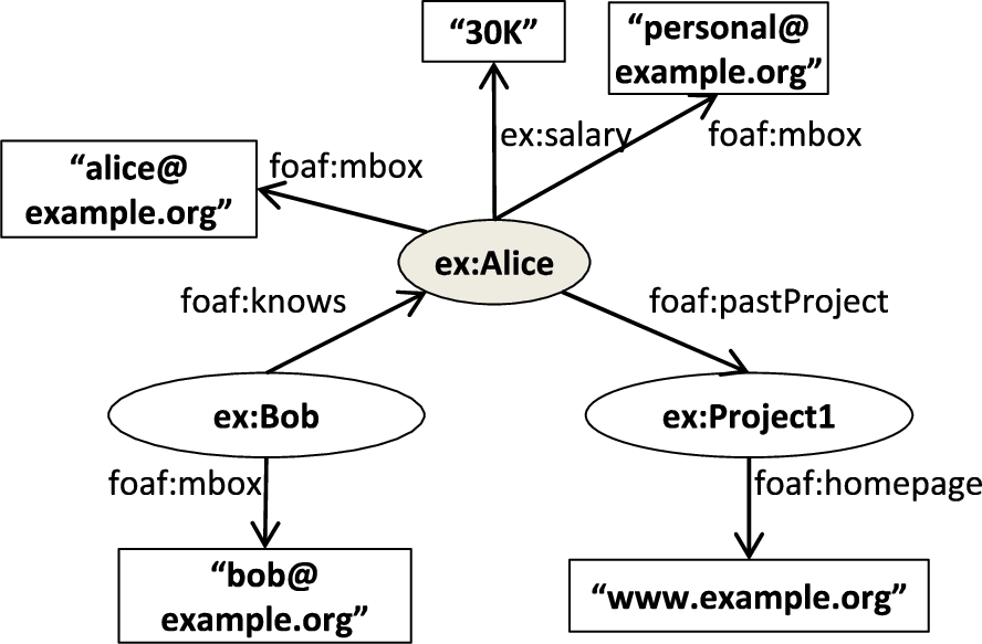
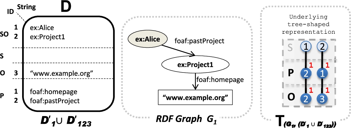
Example of an RDF graph G.

Fig. 2.

HDT Dictionary and Triples for our full graph G.

HDT [10] is a binary, compressed serialization format for optimized RDF storage and transmission, which also allows certain lookups and queries over compressed data. It is therefore very suitable for the efficient exchange and querying of large datasets. HDT encodes an RDF graph G into three components: the Header component H holds metadata, including relevant information necessary for discovery and parsing; the Dictionary component D is a catalogue that encodes all RDF terms in G and maps each of them to a unique identifier; the Triple component T compactly encodes G’s graph structure as tuples of three IDs that are used to represent the directed labelled edges in an RDF graph.

Figure 2 shows the Dictionary component (a), the underlying graph structure (b) and the final Triple component (c) for the previous RDF graph G (Fig. 1).

3.1. HDT dictionary component D

This component organises the terms in a graph G according to their positions in RDF triples, thus we also write $\mathit{D}\mathrm{(}\mathit{G}\mathrm{)}$ to denote the dictionary component constructed from graph G: the section SO manages terms occurring both as subject and object, and maps them to the ID-range [1, |SO|], where |SO| is the number of such terms acting as subject and object. Sections S and O comprise terms that only occur as subjects or objects, respectively. Both sections are mapped from |SO|+1, ranging up to |SO|+|S| and |SO|+|O|, respectively. Finally, section P organises all predicate terms, which are mapped to the range [1, |P|]. It is worth noting that no ambiguity is possible once we know the role (i.e. the position in a triple, being subject, predicate or object) played by the corresponding ID. For further details, we refer to [26]. For convenience, we write $\mathit{id}\mathrm{(}\mathit{x}\mathrm{,}\mathit{D}\mathrm{)}$ for the particular ID assigned to an RDF term x, whereas we refer to all IDs and RDF terms mapped in a dictionary component D as $\mathit{ids}\mathrm{(}\mathit{D}\mathrm{)}$ and $\mathit{terms}\mathrm{(}\mathit{D}\mathrm{)}$ , respectively. Note that, for simplicity, we omit the “role” parameter in these functions, which should be provided in case the terms in subjects (or objects) and predicates are not disjoint [26]. Also, it is worth mentioning that in the original HDT proposal, blank nodes are treated exactly as any other term [10], considering an optional skolemization of blank nodes as a pre-processing step.

3.2. HDT triple component T

This component encodes the structure of the RDF graph after ID substitution, taking into consideration a particular dictionary D, thus, we write $\mathit{T}\mathrm{(}\mathit{G}\mathrm{,}\mathit{D}\mathrm{)}$ to denote a triple component that was constructed from the triples in G using the IDs in dictionary D. More concretely, RDF triples are encoded as groups of three IDs: (id _s id _p id _o ), where id _s , id _p , and id _o are the IDs of the corresponding subject, predicate, and object terms in the dictionary. T organises all triples into a forest of trees, one per different subject: the subject is the root; the middle level comprises the ordered list of predicates reachable from the corresponding subject; and the leaves list the object IDs related to each (subject, predicate) pair. This underlying representation (illustrated in Fig. 2(b)) is effectively encoded following the BitmapTriples approach [10]. It comprises two sequences: Sp and So, concatenating all predicate IDs in the middle level and all object IDs in the leaves, respectively; and two bitsequences: Bp and Bo, which are aligned with Sp and So respectively, using a 1-bit to mark the end of each list (Fig. 2(c)). In practice, each ID in Sp and So is encoded with a fixed-length encoding, using $log\mathrm{(}\mathit{n}\mathrm{)}$ bits, where n is the maximum ID in the sequence [10]. Again, we use $\mathit{ids}\mathrm{(}\mathit{T}\mathrm{)}$ to refer to all IDs used in a triple component T.

3.3. HDT header component H

The HDT Header includes (i) the machine-readable metadata that is necessary to process an HDT file (format metadata); and (ii) additional human-readable information to describe the dataset (usually in the form of VoID1

¹

http://www.w3.org/TR/void/

descriptions). The format metadata is mainly focused on characterising the dictionary and triple formats. In general, an HDT file of a graph G consists of a single header H, dictionary D and triples T, $\mathrm{HDT}\mathrm{(}\mathit{G}\mathrm{)}=\mathrm{(}\mathit{H}\mathrm{,}\mathit{D}\mathrm{,}\mathit{T}\mathrm{)}$ . Nonetheless, the HDT specification [9] is flexible and allows for several dictionaries or triple components to be specified in H as soon as the interpretation of their relationship is provided in the header. It was envisaged that this would be used to split huge RDF graphs into several chunks or streams, where a sequential order of the components is assumed by default [9]. In the following section we exploit and expand this feature to encode a partition of the graph G with several dictionaries and triples.

Fig. 3.

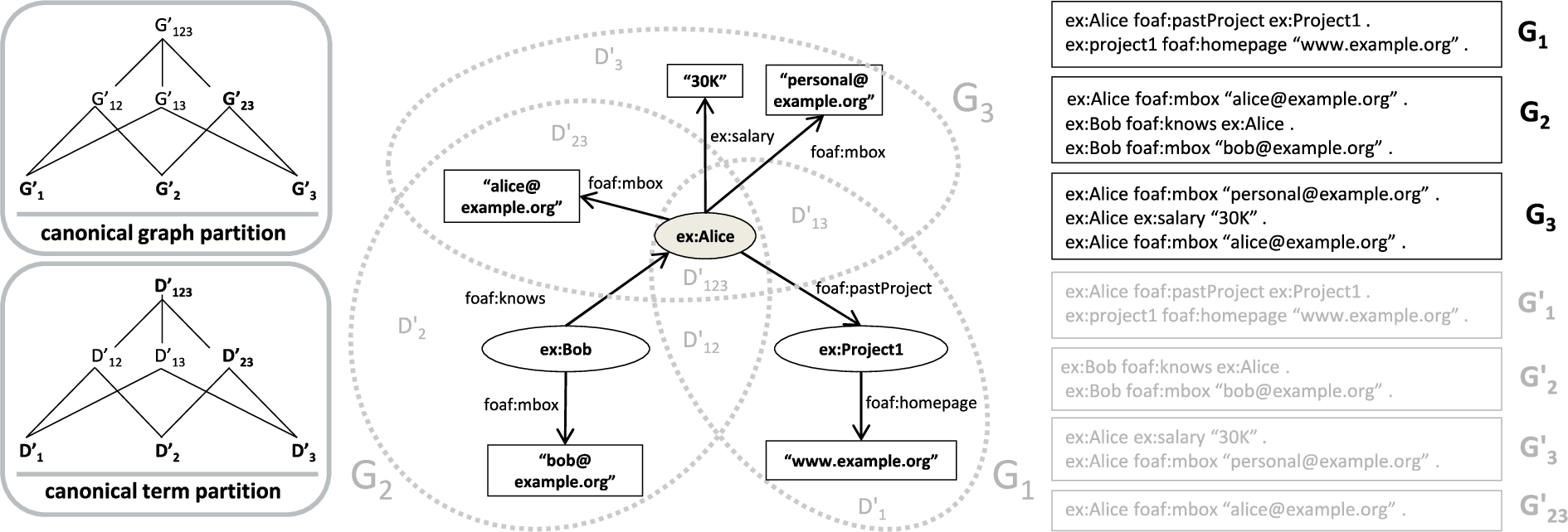
An access-restricted RDF dataset such that G comprises three separate access-restricted subgraphs ${\mathit{G}}_1$ , ${\mathit{G}}_2$ , ${\mathit{G}}_3$ ; the graph’s canonical partition is comprised of four non-empty subgraphs ${\mathit{G}}_1^{\prime }$ , ${\mathit{G}}_2^{\prime }$ , ${\mathit{G}}_3^{\prime }$ , ${\mathit{G}}_{23}^{\prime }$ , whereas the terms in these graphs can be partitioned into five non-empty subsets corresponding to the dictionaries ${\mathit{D}}_1^{\prime }$ , ${\mathit{D}}_2^{\prime }$ , ${\mathit{D}}_3^{\prime }$ , ${\mathit{D}}_{23}^{\prime }$ , ${\mathit{D}}_{123}^{\prime }$ .

4. ${\mathrm{HDT}}_{\mathit{crypt}}$ : Extending HDT for encryption

We introduce ${\mathrm{HDT}}_{\mathit{crypt}}$ , an extension of HDT that involves encryption of RDF graphs. We first define the notion of access-restricted RDF datasets and the implications for HDT (Section 4.1). Then, we show an extension of the HDT header component to cope with access-restricted RDF datasets (Section 4.2), which leads to the final ${\mathrm{HDT}}_{\mathit{crypt}}$ encoding. Finally, as ${\mathrm{HDT}}_{\mathit{crypt}}$ can manage several HDT Dictionary components, we describe the required operations to integrate different Dictionary components within an HDT collection (Section 4.3). These operations will be the basis to represent the shared components between access-restricted datasets efficiently, addressed in Section 5.

4.1. Representing access-restricted RDF datasets

We consider hereinafter that users wishing to publish access-restricted RDF datasets divide their complete graph of RDF triples G into (named) graphs, that are accessible to other users, i.e. we assume that access rights are already materialised per user group in the form of a set (cover) of separate, possibly overlapping, RDF graphs, each of which are accessible to different sets of users.

Borrowing terminology from [17], an access restricted RDF dataset (or just “dataset” in the following) is a set $\mathit{DS}=\{\mathit{G}\mathrm{,}\mathrm{(}{\mathit{g}}_1\mathrm{,}{\mathit{G}}_1\mathrm{)}\mathrm{,}\dots \mathrm{,}\mathrm{(}{\mathit{g}}_{\mathit{n}}\mathrm{,}{\mathit{G}}_{\mathit{n}}\mathrm{)}\}$ consisting of a (non-named) default graph G and named graphs s.t. ${\mathit{g}}_{\mathit{i}}\in \mathit{I}$ are graph names, where in our setting we require that $\{{\mathit{G}}_1\mathrm{,}\dots \mathrm{,}{\mathit{G}}_{\mathit{n}}\}$ is a cover2

²

In the set-theoretic sense.

of G. We further call $\mathit{DS}$ a partition of G if ${\mathit{G}}_{\mathit{i}}\cap {\mathit{G}}_{\mathit{j}}=\varnothing$ for any $\mathit{i}\ne \mathit{j}$ ; $1⩽\mathit{i}\mathrm{,}\mathit{j}⩽\mathit{n}$ . Note that from any dataset $\mathit{DS}$ , a canonical partition ${\mathit{DS}}^{\prime }$ can be trivially constructed (but may be exponential in size) consisting of all non-empty (at most $2^{\mathit{n}}-1$ ) subsets ${\mathit{G}}_{\mathit{S}}^{\prime }$ of triples $\mathit{t}\in \mathit{G}$ corresponding to an index set $\mathit{S}\in 2^{1\mathrm{,}\dots \mathrm{,}\mathit{i}}$ such that ${\mathit{G}}_{\mathit{S}}^{\prime }=\{\mathit{t}\mid \mathit{t}\in {\bigcap }_{\mathit{i}\in \mathit{S}}{\mathit{G}}_{\mathit{i}}\wedge \neg \exists {\mathit{S}}^{\prime }:\mathrm{(}{\mathit{S}}^{\prime }\supset \mathit{S}\wedge \mathit{t}\in {\bigcap }_{\mathit{j}\in {\mathit{S}}^{\prime }}{\mathit{G}}_{\mathit{j}}\mathrm{)}\}$ .

Figure 3 shows an example of such a dataset composed of three access-restricted subgraphs (or just “subgraphs” in the following) ${\mathit{G}}_1$ , ${\mathit{G}}_2$ , ${\mathit{G}}_3$ for the previous full graph G (Fig. 2(a)). Intuitively, this corresponds to a scenario with three access rights: users who can access general information about projects in an organisation (graph ${\mathit{G}}_1$ ); users who have access to public email accounts and relations between members in the organisation (graph ${\mathit{G}}_2$ ); and finally, users who can view personal information of members, such as the salary and personal email accounts (graph ${\mathit{G}}_3$ ). As can be seen, the triple (ex:Alice foaf:mbox “[e-mail]”) is repeated in subgraphs ${\mathit{G}}_2$ and ${\mathit{G}}_3$ , showing a redundancy which can produce significant overheads in realistic scenarios with large-scale datasets and highly overlapping graphs. Canonical partitioning groups these triples into disjoint sets so that no repetitions are present. In our example in Fig. 3, the set ${\mathit{G}}_{\{2\mathrm{,}3\}}^{\prime }$ , which can simply be written as ${\mathit{G}}_{23}^{\prime }$ , holds this single triple, (ex:Alice foaf:mbox “[e-mail]”), hence this triple is not present in ${\mathit{G}}_2^{\prime }$ and ${\mathit{G}}_3^{\prime }$ . In this simple scenario, ${\mathit{G}}_1^{\prime }$ is equivalent to ${\mathit{G}}_1$ as it does not share triples with other graphs.

Thus, we consider hereinafter an HDT collection corresponding to a dataset $\mathit{DS}$ denoted by $\mathrm{HDT}\mathrm{(}\mathit{DS}\mathrm{)}=\mathrm{(}\mathit{H}\mathrm{,}\mathcal{D}\mathrm{,}\mathcal{T}\mathrm{)}$ as a single H, plus sets $\mathcal{D}=\{{\mathit{D}}_1\mathrm{,}\dots \mathrm{,}{\mathit{D}}_{\mathit{n}}\}$ , $\mathcal{T}=\{{\mathit{T}}_1\mathrm{,}\dots \mathrm{,}{\mathit{T}}_{\mathit{m}}\}$ of dictionary and triple components, respectively, such that the union of triple components encodes a cover of G, i.e. the overall graph of all triples in the dataset $\mathit{DS}$ . We do not assume that there is a one-to-one correspondence between individual triple components in $\mathcal{T}$ and graphs in $\mathit{DS}$ ; different options of mapping subgraphs to HDT components will be discussed in Section 5 below. The relation between the dictionaries and the triple components (in other words, which dictionaries are used to codify which triple components) is also flexible and must be specified through metadata properties. In our case, we assume $\mathit{H}=\{\mathit{R}\mathrm{,}\mathit{M}\}$ to contain a relation $\mathit{R}\subseteq \mathcal{D}\times \mathcal{T}$ , which we call the dictionary-triples map with the implicit meaning that dictionary components encode terms used in the corresponding triple components, and M is comprised of additional header metadata (as mentioned above, the header contains a variety of further (meta-)information in standard HDT [9], which we skip for the considerations herein). It is worth noting that we do not prescribe that either D or T do not overlap. However, it is clear that one should find an unambiguous correspondence to decode the terms under $\mathit{ids}\mathrm{(}\mathit{T}\mathrm{)}$ .

Thus, we define the following admissibility condition for R. An HDT collection is called admissible if:

• $\forall {\mathit{D}}_{\mathit{i}}\mathrm{,}{\mathit{D}}_{\mathit{j}}\in \mathcal{D}:\mathrm{(}{\mathit{D}}_{\mathit{i}}\mathrm{,}\mathit{T}\mathrm{)}\mathrm{,}\mathrm{(}{\mathit{D}}_{\mathit{j}}\mathrm{,}\mathit{T}\mathrm{)}\in \mathit{R}\wedge \mathit{i}\ne \mathit{j}⟹\mathit{terms}\mathrm{(}{\mathit{D}}_{\mathit{i}}\mathrm{)}\cap \mathit{terms}\mathrm{(}{\mathit{D}}_{\mathit{j}}\mathrm{)}=\varnothing$

• $\forall \mathit{T}\in \mathcal{T}:\mathit{i}\in \mathit{ids}\mathrm{(}\mathit{T}\mathrm{)}⟹\exists \mathrm{(}\mathit{D}\mathrm{,}\mathit{T}\mathrm{)}\in \mathit{R}\wedge \mathit{i}\in \mathit{ids}\mathrm{(}\mathit{D}\mathrm{)}$

For any admissible HDT collection $\mathrm{HDT}$ we define the T-restricted collection ${\mathrm{HDT}}^{\mathit{T}}$ as the collection obtained from removing: (i) all triple components ${\mathit{T}}^{\prime }\ne \mathit{T}$ from $\mathrm{HDT}$ ; (ii) the corresponding ${\mathit{D}}^{\prime }$ such that $\mathrm{(}{\mathit{D}}^{\prime }\mathrm{,}{\mathit{T}}^{\prime }\mathrm{)}$ is in R and $\mathrm{(}{\mathit{D}}^{\prime }\mathrm{,}\mathit{T}\mathrm{)}$ is not in R; and (iii) the relations $\mathrm{(}{\mathit{D}}^{\prime }\mathrm{,}{\mathit{T}}^{\prime }\mathrm{)}$ from R. Thus allowing an HDT collection to be filtered by erasing all dictionary and triple components that are not required for T.

4.2. ${\mathrm{HDT}}_{\mathit{crypt}}$ encoding

We now introduce the final encoding of the ${\mathrm{HDT}}_{\mathit{crypt}}$ extension. ${\mathrm{HDT}}_{\mathit{crypt}}$ uses AES (Advanced Encryption Standard) [7] to encrypt the D and triple components of an HDT collection and extends the header H with a keymap $\mathit{kmap}:{\mathcal{D}}_{\mathit{crypt}}\cup {\mathcal{T}}_{\mathit{crypt}}\mapsto \mathit{I}$ that maps encrypted components to identifiers (IRIs), which denote AES keys that can be used to decrypt these components.

Thus, ${\mathrm{HDT}}_{\mathit{crypt}}=\mathrm{(}\mathit{H}\mathrm{,}{\mathcal{D}}_{\mathit{crypt}}\mathrm{,}{\mathcal{T}}_{\mathit{crypt}}\mathrm{)}$ where $\mathit{H}=\{\mathit{R}\mathrm{,}\mathit{kmap}\mathrm{,}\mathit{M}\}$ , $\mathit{R}\subseteq {\mathcal{D}}_{\mathit{crypt}}\times {\mathcal{T}}_{\mathit{crypt}}$ , and the components in ${\mathcal{D}}_{\mathit{crypt}}$ and ${\mathcal{T}}_{\mathit{crypt}}$ are encrypted with keys identified in $\mathit{kmap}$ .

The operations to $\mathit{encrypt}$ and $\mathit{decrypt}$ the dictionary and triples are described as follows. First, the operation $\mathit{encrypt}$ takes one or more dictionary and triples and encrypts the components with a given key. Formally, we write $\mathit{encrypt}\mathrm{(}\mathit{c}\mathrm{,}{\mathit{key}}_{\mathit{crypt}}\mathrm{)}={\mathit{c}}_{\mathit{crypt}}$ , where $\mathit{c}\in \mathcal{D}\cup \mathcal{T}$ to denote the component ${\mathit{c}}_{\mathit{crypt}}\in {\mathcal{D}}_{\mathit{crypt}}\cup {\mathcal{T}}_{\mathit{crypt}}$ obtained by encrypting c with the key ${\mathit{key}}_{\mathit{crypt}}$ . While, we add an identifier of the components to the header metadata. In other words, $\mathit{id}\mathrm{(}{\mathit{c}}_{\mathit{crypt}}\mathrm{)}\mapsto \mathit{IRI}\mathrm{(}{\mathit{key}}_{\mathit{crypt}}\mathrm{)}$ is added to the kmap, where $\mathit{id}$ denotes the ID of the component in ${\mathcal{D}}_{\mathit{crypt}}$ and ${\mathcal{T}}_{\mathit{crypt}}$ and $\mathit{IRI}$ a unique identifier for the symmetric key.

For the decryption, it is assumed that an authorized user u has partial knowledge about these keys, i.e. they have access to a partial function ${\mathit{key}}_{\mathit{u}}:{\mathit{I}}_{\mathit{u}}\mapsto \mathit{K}$ that maps a finite set of “user-owned” key IDs ${\mathit{I}}_{\mathit{u}}\subseteq \mathit{I}$ to the set of AES (symmetric) keys K. The decryption simply takes the given compressed component(s) and performs the decryption with the given symmetric key. Formally, we write $\mathit{decrypt}\mathrm{(}{\mathit{c}}_{\mathit{crypt}}\mathrm{,}{\mathit{key}}_{\mathit{crypt}}\mathrm{)}=\mathit{c}$ , where ${\mathit{c}}_{\mathit{crypt}}\in {\mathcal{D}}_{\mathit{crypt}}\cup {\mathcal{T}}_{\mathit{crypt}}$ to denote the component $\mathit{c}\in \mathcal{D}\cup \mathcal{T}$ obtained from decrypting ${\mathit{c}}_{\mathit{crypt}}$ with the key ${\mathit{key}}_{\mathit{crypt}}=\mathit{key}\mathrm{(}\mathit{kmap}\mathrm{(}{\mathit{c}}_{\mathit{crypt}}\mathrm{)}\mathrm{)}$ . Further we write $\mathit{decrypt}\mathrm{(}{\mathrm{HDT}}_{\mathit{crypt}}\mathrm{,}{\mathit{I}}_{\mathit{u}}\mathrm{)}$ to denote the non-encrypted HDT collection consisting of all decrypted dictionary and triple components of ${\mathrm{HDT}}_{\mathit{crypt}}$ which can be decrypted with the keys in $\{{\mathit{key}}_{\mathit{u}}\mathrm{(}\mathit{i}\mathrm{)}\mid \mathit{i}\in {\mathit{I}}_{\mathit{u}}\}$ . In other words, the T-restriction of ${\mathrm{HDT}}_{\mathit{crypt}}$ is defined analogously to the above-said.

4.3. Integration operations

Finally, we define two different ways of integrating dictionaries ${\mathit{D}}_1\mathrm{,}\dots \mathrm{,}{\mathit{D}}_{\mathit{k}}\in \mathcal{D}$ within an HDT collection: D-union and D-merge. In the former, we replace dictionaries with a new dictionary that includes the union of all terms. In the latter, we establish one of the dictionaries as the dictionary baseline and rename the IDs of the other dictionaries.

4.3.1. D-Union

The D-union is only defined for ${\mathit{D}}_1\mathrm{,}\dots \mathrm{,}{\mathit{D}}_{\mathit{k}}\subseteq \mathcal{D}$ if the following condition holds on R: $\forall \mathrm{(}{\mathit{D}}_{\mathit{i}}\mathrm{,}\mathit{T}\mathrm{)}\in \mathit{R}:\mathrm{(}\neg \exists {\mathit{D}}_{\mathit{j}}\notin {\mathit{D}}_1\mathrm{,}\dots \mathrm{,}{\mathit{D}}_{\mathit{k}}\text{ such that }\mathrm{(}{\mathit{D}}_{\mathit{j}}\mathrm{,}\mathit{T}\mathrm{)}\in \mathit{R}\mathrm{)}$ . In other words, we can perform a D-union if all T-components depending on dictionaries in the set ${\mathit{D}}_1\mathrm{,}\dots \mathrm{,}{\mathit{D}}_{\mathit{k}}$ only depend on these dictionaries. Then, we can define a trivial D-union of $\mathrm{HDT}$ wrt. ${\mathit{D}}_1\mathrm{,}\dots \mathrm{,}{\mathit{D}}_{\mathit{k}}$ , written ${\mathrm{HDT}}_{{\mathit{D}}_1\cup \cdots \cup {\mathit{D}}_{\mathit{k}}}$ , as follows:

replace $\{{\mathit{D}}_1\mathrm{,}\dots \mathrm{,}{\mathit{D}}_{\mathit{k}}\}$ dictionaries with a single dictionary ${\mathit{D}}_{1\dots \mathit{k}}={\mathit{D}}_1\cup \cdots \cup {\mathit{D}}_{\mathit{k}}$ , such that $\forall \mathit{x}\in \mathit{terms}\mathrm{(}{\mathit{D}}_1\mathrm{)}\cup \cdots \cup \mathit{terms}\mathrm{(}{\mathit{D}}_{\mathit{k}}\mathrm{)}$

• $\mathit{x}\in \mathit{terms}\mathrm{(}{\mathit{D}}_{1\dots \mathit{k}}\mathrm{)}$

• $\mathit{id}\mathrm{(}\mathit{x}\mathrm{,}{\mathit{D}}_{1\dots \mathit{k}}\mathrm{)}$ is obtained by sequentially numbering the terms in $\mathit{terms}\mathrm{(}{\mathit{D}}_1\mathrm{)}\cup \cdots \cup \mathit{terms}\mathrm{(}{\mathit{D}}_{\mathit{k}}\mathrm{)}$ upon an (arbitrary) total order, e.g., lexicographically ordering the terms (as it is done in HDT dictionaries by default).

replace all $\mathrm{(}{\mathit{D}}_{\mathit{i}}\mathrm{,}\mathit{T}\mathrm{)}\in \mathit{R}$ , $\mathit{i}\in \{1\mathrm{,}\dots \mathrm{,}\mathit{k}\}$ , with new $\mathrm{(}{\mathit{D}}_{1\dots \mathit{k}}\mathrm{,}{\mathit{T}}^{\prime }\mathrm{)}$ relations, where ${\mathit{T}}^{\prime }$ is obtained from T by replacing the original IDs from ${\mathit{D}}_{\mathit{i}}$ with their corresponding new IDs in ${\mathit{D}}_{1\dots \mathit{k}}$ .

4.3.2. D-Merge

In the more general case where the condition for D-unions does not hold on ${\mathit{D}}_1\mathrm{,}\dots \mathrm{,}{\mathit{D}}_{\mathit{k}}\subseteq \mathcal{D}$ , then we can define another operation, D-merge, written ${\mathrm{HDT}}_{{\mathit{D}}_1⊳\cdots ⊳{\mathit{D}}_{\mathit{k}}}$ . We start with the binary case, where only two dictionaries ${\mathit{D}}_1$ and ${\mathit{D}}_2$ are involved; ${\mathrm{HDT}}_{{\mathit{D}}_1⊳{\mathit{D}}_2}$ is obtain as follows:

replace ${\mathit{D}}_1$ and ${\mathit{D}}_2$ with a single ${\mathit{D}}_{12}={\mathit{D}}_1⊳{\mathit{D}}_2$ ,3

³

We use the directed operator ⊳ instead of ∪ here, since this operation is not commutative.

such that

• $\forall \mathit{x}\in \mathit{terms}\mathrm{(}{\mathit{D}}_1\mathrm{)}:\mathit{id}\mathrm{(}\mathit{x}\mathrm{,}{\mathit{D}}_{12}\mathrm{)}=\mathit{id}\mathrm{(}\mathit{x}\mathrm{,}{\mathit{D}}_1\mathrm{)}$

• $\forall \mathit{x}\in \mathit{terms}\mathrm{(}{\mathit{D}}_2\mathrm{)}\setminus \mathit{terms}\mathrm{(}{\mathit{D}}_1\mathrm{)}:\mathit{id}\mathrm{(}\mathit{x}\mathrm{,}{\mathit{D}}_{12}\mathrm{)}=\mathit{id}\mathrm{(}\mathit{x}\mathrm{,}{\mathit{D}}_2\mathrm{)}+max\mathrm{(}\mathit{ids}\mathrm{(}{\mathit{D}}_1\mathrm{)}\mathrm{)}$

replace all $\mathrm{(}{\mathit{D}}_1\mathrm{,}{\mathit{T}}_1\mathrm{)}\in \mathit{R}$ with $\mathrm{(}{\mathit{D}}_{12}\mathrm{,}{\mathit{T}}_1\mathrm{)}$

replace all $\mathrm{(}{\mathit{D}}_2\mathrm{,}{\mathit{T}}_2\mathrm{)}\in \mathit{R}$ with $\mathrm{(}{\mathit{D}}_{12}\mathrm{,}{\mathit{T}}_2^{\prime }\mathrm{)}$ , where ${\mathit{T}}_2^{\prime }$ is obtained from ${\mathit{T}}_2$ by analogous ID changes.

D-merge can then be generalized to a sequence of dictionaries assuming left-associativity of ⊳ operator, i.e. ${\mathrm{HDT}}_{{\mathit{D}}_1⊳{\mathit{D}}_2⊳\cdots ⊳{\mathit{D}}_{\mathit{k}}}={\mathrm{HDT}}_{\mathrm{(}\mathrm{(}{\mathit{D}}_1⊳{\mathit{D}}_2\mathrm{)}⊳\cdots \mathrm{)}⊳{\mathit{D}}_{\mathit{k}}}$ .

For convenience, we extend the notation of $\mathit{T}\mathrm{(}\mathit{G}\mathrm{,}\mathit{D}\mathrm{)}$ from Section 3.2 to D-unions and D-merges: let $\mathrm{(}{\mathit{D}}_1\mathrm{,}\dots \mathrm{,}{\mathit{D}}_{\mathit{k}}\mathrm{)}$ be a sequence of dictionaries and G an RDF graph such that $\mathit{terms}\mathrm{(}\mathit{G}\mathrm{)}={\bigcup }_{{\mathit{D}}_{\mathit{i}}\in \mathrm{(}{\mathit{D}}_1\mathrm{,}\dots \mathrm{,}{\mathit{D}}_{\mathit{k}}\mathrm{)}}\mathit{terms}\mathrm{(}{\mathit{D}}_{\mathit{i}}\mathrm{)}$ . Then we will write $\mathit{T}\mathrm{(}\mathit{G}\mathrm{,}\mathrm{(}{\mathit{D}}_1\cup \cdots \cup {\mathit{D}}_{\mathit{k}}\mathrm{)}\mathrm{)}$ and $\mathit{T}\mathrm{(}\mathit{G}\mathrm{,}\mathrm{(}{\mathit{D}}_1⊳\cdots ⊳{\mathit{D}}_{\mathit{k}}\mathrm{)}\mathrm{)}$ for the triples part generated from G according to the combined dictionary $\mathrm{(}\mathrm{(}{\mathit{D}}_1\cup {\mathit{D}}_2\mathrm{)}\cup \cdots \mathrm{)}\cup {\mathit{D}}_{\mathit{k}}$ and $\mathrm{(}\mathrm{(}{\mathit{D}}_1⊳{\mathit{D}}_2\mathrm{)}⊳\cdots \mathrm{)}⊳{\mathit{D}}_{\mathit{k}}$ respectively. Finally, we note that for any admissible HDT collection, both D-union and D-merge preserve admissibility.

5. Efficient partitioning ${\mathrm{HDT}}_{\mathit{crypt}}$

After having introduced the general idea of ${\mathrm{HDT}}_{\mathit{crypt}}$ and the two different ways of integrating dictionaries within an HDT collection, we now discuss four alternatives strategies that can be used for distributing a dataset $\mathit{DS}$ across dictionary and triple components in an ${\mathrm{HDT}}_{\mathit{crypt}}$ collection. These alternatives, referred to as HDT _crypt-A , HDT _crypt-B , HDT _crypt-C and HDT _crypt-D , provide different space/performance tradeoffs that will be evaluated in Section 6. We note that HDT behaves differently than the normal RDF merge regarding blank nodes in different “partitions” as, by default, HDT does not rename the blank nodes to avoid shared labels [19]: the original blank nodes are skolemized to constants (unique per RDF graph) and preserved across partitions, so that we do not need to consider blank node (re-)naming separately.

5.1. HDT _crypt-A : A dictionary and triples per named graph in $\mathit{DS}$

The baseline approach is straightforward, we construct separate HDT components ${\mathit{D}}_{\mathit{i}}=\mathit{D}\mathrm{(}{\mathit{G}}_{\mathit{i}}\mathrm{)}$ and ${\mathit{T}}_{\mathit{i}}=\mathit{T}\mathrm{(}{\mathit{G}}_{\mathit{i}}\mathrm{,}{\mathit{D}}_{\mathit{i}}\mathrm{)}$ per graph ${\mathit{G}}_{\mathit{i}}$ in the dataset, see Fig. 4, thereafter each of these components is encrypted with a respective, separate key, identified by a unique IRI ${\mathit{id}}_{\mathit{i}}\in \mathit{I}$ , i.e., $\mathit{kmap}\mathrm{(}{\mathit{D}}_{\mathit{i}}\mathrm{)}=\mathit{kmap}\mathrm{(}{\mathit{T}}_{\mathit{i}}\mathrm{)}={\mathit{id}}_{\mathit{i}}$ and $\mathit{R}=\{\mathrm{(}{\mathit{D}}_{\mathit{i}}\mathrm{,}{\mathit{T}}_{\mathit{i}}\mathrm{)}\mid {\mathit{G}}_{\mathit{i}}\in \mathit{DS}\}$ . For re-obtaining graph ${\mathit{G}}_{\mathit{i}}$ a user must only have access to the key corresponding to ${\mathit{id}}_{\mathit{i}}$ , and can thereby decrypt ${\mathit{D}}_{\mathit{i}}$ and ${\mathit{T}}_{\mathit{i}}$ and extract the restricted collection ${\mathrm{HDT}}^{{\mathit{T}}_{\mathit{i}}}$ , which corresponds to ${\mathit{G}}_{\mathit{i}}$ . Obviously, this approach encodes a lot of overlaps in both dictionary and triples parts: that is, for our running example from Fig. 4, the IRI for ex:alice is encoded in each individual D component and the overlapping triples in graphs ${\mathit{G}}_2$ and ${\mathit{G}}_3$ appear in both ${\mathit{T}}_2$ and ${\mathit{T}}_3$ respectively (cf., Fig. 4).

Fig. 4.

HDT _crypt-A , create and encrypt one HDT per partition.

Fig. 5.

HDT _crypt-B , extracting non-overlapping triples.

5.2. HDT _crypt-B : Extracting non-overlapping triples in ${\mathit{DS}}^{\prime }$

In order to avoid the overlaps in the triple components, a more efficient approach could be to split the graphs in the dataset $\mathit{DS}$ according to their canonical partition ${\mathit{DS}}^{\prime }$ and again construct separate (D, T)-pairs for each subset ${\mathit{G}}_{\mathit{S}}^{\prime }\in {\mathit{DS}}^{\prime }$ , see Fig. 5. That is, we create ${\mathit{D}}_{\mathit{S}}^{\prime }=\mathit{D}\mathrm{(}{\mathit{G}}_{\mathit{S}}^{\prime }\mathrm{)}$ and ${\mathit{T}}_{\mathit{S}}^{\prime }=\mathit{T}\mathrm{(}{\mathit{G}}_{\mathit{S}}^{\prime }\mathrm{,}{\mathit{D}}_{\mathit{S}}^{\prime }\mathrm{)}$ per graph ${\mathit{G}}_{\mathit{S}}^{\prime }\in {\mathit{DS}}^{\prime }$ , where $\mathit{S}\in 2^{1\mathrm{,}\dots \mathrm{,}\mathit{i}}$ denotes the index set corresponding to a (non-empty) subset of ${\mathit{DS}}^{\prime }$ . R in turn contains pairs $\mathrm{(}{\mathit{D}}_{\mathit{S}}^{\prime }\mathrm{,}{\mathit{T}}_{\mathit{S}}^{\prime }\mathrm{)}$ and $\mathit{kmap}$ entries for keys identified by ${\mathit{I}}_{\mathit{S}}^{\prime }$ per ${\mathit{G}}_{\mathit{S}}^{\prime }$ used for the encryption/decryption of the relevant ${\mathit{D}}_{\mathit{S}}^{\prime }$ and ${\mathit{T}}_{\mathit{S}}^{\prime }$ . The difference for decryption now is that any user who is allowed access to ${\mathit{G}}_{\mathit{i}}$ must have all keys corresponding to any ${\mathit{I}}_{\mathit{S}}^{\prime }$ such that $\mathit{i}\in \mathit{S}$ in order to re-obtain the original graph ${\mathit{G}}_{\mathit{i}}$ .

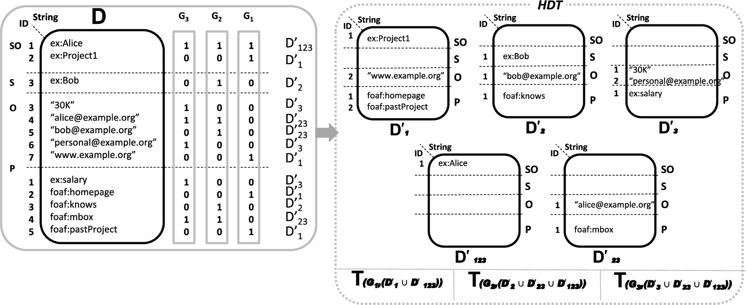
First, the user will decrypt all the components for which they have keys, i.e. obtaining a non-encrypted collection ${\mathrm{HDT}}^{\prime }$ consisting of components ${\mathcal{D}}^{\prime }=\{{\mathit{D}}_1^{\prime }\mathrm{,}\dots \mathrm{,}{\mathit{D}}_{\mathit{k}}^{\prime }\}$ , ${\mathcal{T}}^{\prime }=\{{\mathit{T}}_1^{\prime }\mathrm{,}\dots \mathrm{,}{\mathit{T}}_{\mathit{k}}^{\prime }\}$ consisting of the components corresponding to a partition of ${\mathit{G}}_{\mathit{i}}$ . Then, for decompressing the original graph ${\mathit{G}}_{\mathit{i}}$ , we create separate ${\mathit{T}}_{\mathit{S}}^{\prime }$ -restricted HDTs, which are decompressed separately, with ${\mathit{G}}_{\mathit{S}}$ being the union of the resulting subgraphs.

Fig. 6.

HDT _crypt-C , extracting non-overlapping dictionaries.

Fig. 7.

Union of dictionaries (in HDT _crypt-C ) to codify the non-overlapping dictionaries of a partition.

5.3. HDT _crypt-C : Extracting non-overlapping dictionaries in ${\mathit{DS}}^{\prime }$

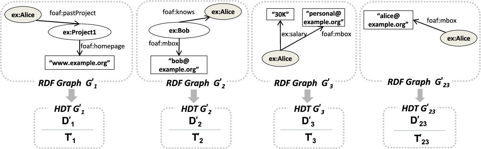
Note that in the previous approach, we have duplicates in the dictionary components. An alternative strategy would be to create a canonical partition of terms instead of triples, and create separate dictionaries ${\mathit{D}}_{\mathit{S}}^{\prime }\in {\mathcal{D}}^{\prime }$ for each non-empty term-subset,4

⁴

Again, here $\mathit{S}\in 2^{1\mathrm{,}\dots \mathrm{,}\mathit{n}}$ represents an index set.

respectively. Figure 6 shows the canonical partition of terms in our running example: as can be seen, the original dictionary is split into five non-empty terms-subsets corresponding to the dictionaries ${\mathit{D}}_{123}^{\prime }$ (terms shared in all three graphs), ${\mathit{D}}_{23}^{\prime }$ (terms shared in graphs ${\mathit{G}}_2$ and ${\mathit{G}}_3$ that are not in ${\mathit{D}}_{123}^{\prime }$ ) and ${\mathit{D}}_1^{\prime }$ , ${\mathit{D}}_2^{\prime }$ , ${\mathit{D}}_3^{\prime }$ (terms in either ${\mathit{G}}_1$ , ${\mathit{G}}_2$ or ${\mathit{G}}_3$ resp. and are not shared between graphs). This partition can be computed efficiently, thanks to the HDT dictionary D of the full graph G, which we assume to be available.5 ⁵

All ${\mathrm{HDT}}_{\mathit{crypt}}$ strategies are evaluated from an existing full graph G. Our evaluation in Section 6 also reports the time to create the HDT representation of the full graph G.

To do so, we keep6 ⁶

This auxiliary structure is maintained just at compression time and it is not shipped with the encrypted information.

an auxiliary bitsequence per graph ${\mathit{G}}_{\mathit{i}}$ (see Fig. 6, top left), each of size $\mathit{terms}\mathrm{(}\mathit{D}\mathrm{)}$ . Then, we iterate through triples in each graph ${\mathit{G}}_{\mathit{i}}$ and, for each term, we search its ID in D, marking such position with a 1-bit in the bitsequence of ${\mathit{G}}_{\mathit{i}}$ . Finally, the dictionaries of the subsets can be created by inspecting the combinations of 1-bits in the bitsequences: terms in ${\mathit{D}}_{\mathit{x}\mathit{y}\cdots \mathit{z}}^{\prime }$ will be those with a 1-bit in the bitsequences of graphs $\mathit{x}\mathit{y}\cdots \mathit{z}$ and 0-bits in other graphs. For instance, in Fig. 6, ${\mathit{D}}_{123}^{\prime }$ is constituted only by ex:alice, because it is the only term with three 1-bits in the bitsequences of ${\mathit{G}}_1$ , ${\mathit{G}}_2$ and ${\mathit{G}}_3$ . In contrast, ex:Project1 will be part of ${\mathit{D}}_1^{\prime }$ as it has a 1-bit only in the bitsequence of ${\mathit{G}}_1$ .

The number of triple components in this approach are as in HDT _crypt-A , one per graph ${\mathit{G}}_{\mathit{i}}$ . However, they are constructed slightly differently as, in this case, we have a canonical partition of terms and one user will just receive the dictionaries corresponding to subsets that correspond to terms in the graph ${\mathit{G}}_{\mathit{i}}$ that they have been granted access to. In other words, the IDs used in each ${\mathit{T}}_{\mathit{i}}$ should unambiguously correspond to terms, but these terms may be distributed across several dictionaries.7 ⁷

Given the partition definition, it is nonetheless true that a term appears in one and only one term-subset.

Thus, we encode triples with a D-union (see Section 4.3) of the ${\mathit{D}}_{\mathit{S}}^{\prime }$ such that $\mathit{i}\in \mathit{S}$ . That is, for each ${\mathit{G}}_{\mathit{i}}$ we construct ${\mathit{T}}_{\mathit{i}}=\mathit{T}\mathrm{(}{\mathit{G}}_{\mathit{i}}\mathrm{,}\mathrm{(}{\bigcup }_{\mathit{i}\in \mathit{S}}{\mathit{D}}_{\mathit{S}}^{\prime }\mathrm{)}\mathrm{)}$ , and add the respective pairs $\mathrm{(}{\mathit{D}}_{\mathit{S}}^{\prime }\mathrm{,}{\mathit{T}}_{\mathit{i}}\mathrm{)}$ in R.

Fig. 8.

HDT _crypt-D , extracting non-overlapping dictionaries and triples.

Figure 7 illustrates this merge of dictionaries for the graph ${\mathit{G}}_1$ and the respective construction of $\mathit{T}\mathrm{(}{\mathit{G}}_1\mathrm{,}\mathrm{(}{\mathit{D}}_1^{\prime }\cup {\mathit{D}}_{123}^{\prime }\mathrm{)}\mathrm{)}$ . The decompression process after decryption is the exact opposite. For decompressing the graph ${\mathit{G}}_{\mathit{i}}$ , the decrypted dictionaries ${\bigcup }_{\mathit{i}\in \mathit{S}}{\mathit{D}}_{\mathit{S}}^{\prime }$ are used to create a D-union ${\mathit{D}}_{\mathit{i}}$ which can be used to decompress the triples ${\mathit{T}}_{\mathit{i}}$ in one go. Finally, as a performance improvement at compression time, note that, although the canonical partition of terms has to be built to be shipped in the compressed output, we can actually skip the creation of the D-union dictionaries to encode the IDs in the triples. To do so, we make use of the bitsequences to get the final IDs that are used in the triples: One should note that the ID of a term in a D-union of a graph ${\mathit{G}}_{\mathit{i}}$ is the number of previous 1-bits in the bitsequence of ${\mathit{G}}_{\mathit{i}}$ (for each $\mathit{S}\mathit{O}$ , S, O, and P section). For instance, in our example in Fig. 7, ex:Project1 is encoded with the $\mathrm{ID}=2$ . Instead of creating ${\mathit{D}}_1$ , we can see that in the bitsequence of ${\mathit{G}}_1$ (see Fig. 6, top right) we have two 1-bits in the predicate section up to the position where ex:Project1 is stored in the original dictionary, hence its $\mathrm{ID}=2$ .

5.4. HDT _crypt-D : Extracting non-overlapping dictionaries and triples in ${\mathit{DS}}^{\prime }$

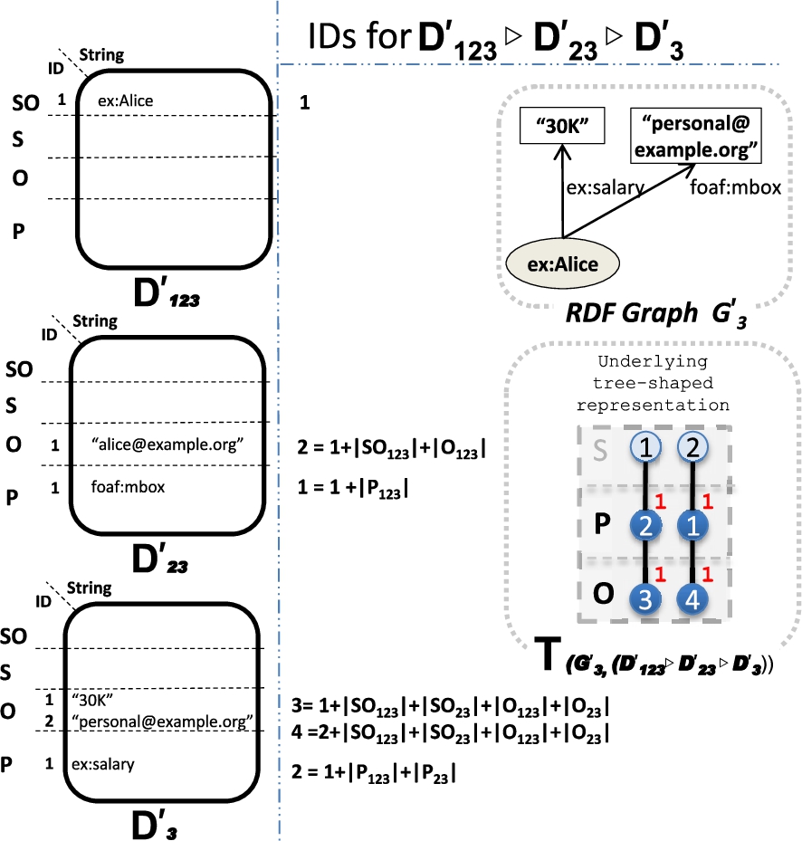
In HDT _crypt-D , we combine the methods of both HDT _crypt-B and HDT _crypt-C . That is, we first create a canonical partition of terms as in HDT _crypt-C , and a canonical partition of triples ${\mathit{DS}}^{\prime }$ as in HDT _crypt-B . Then, we codify the IDs in the subsets of ${\mathit{DS}}^{\prime }$ with the IDs from the dictionaries. Note, however, that in this case there is – potentially – an $\mathit{n}:\mathit{m}$ between the resulting dictionary and triple components. In other words, triples in ${\mathit{T}}_{\mathit{S}}^{\prime }$ can include terms that are not only in ${\mathit{D}}_{\mathit{S}}^{\prime }$ as they may be distributed across several term-subsets. For instance, in our running example, ${\mathit{T}}_1^{\prime }$ in HDT _crypt-B includes ex:Alice (see Fig. 5) which is stored in ${\mathit{D}}_{123}^{\prime }$ in HDT _crypt-C (see Fig. 6). One alternative could be to create a D-union of each graph ${\mathit{G}}_{\mathit{S}}^{\prime }$ and codify triples in ${\mathit{T}}_{\mathit{S}}^{\prime }$ with the corresponding IDs. However, it is trivial to see that this would lead to an exponential number of D-union dictionaries, one per ${\mathit{T}}_{\mathit{S}}^{\prime }$ component. In addition, we would need to physically recreate all these dictionaries at compression time, and also at decompression time in order to decompress each single graph ${\mathit{G}}_{\mathit{S}}^{\prime }$ . Thus, we perform a D-merge approach (see the definition in Section 4.3), which fits perfectly with $\mathit{n}:\mathit{m}$ -relations. This is illustrated in Fig. 8. As can be seen, triples in each ${\mathit{G}}_{\mathit{S}}^{\prime }$ of the canonical partition are encoded with an appropriate D-merge of term-subsets. A practical example is shown in Fig. 9, representing the encoding of graph ${\mathit{G}}_3^{\prime }$ . As defined in D-merge, IDs are assigned in order, that is for a merge ${\mathit{D}}_1^{\prime }⊳\cdots ⊳{\mathit{D}}_{\mathit{k}}^{\prime }$ , the IDs in ${\mathit{D}}_{\mathit{k}}^{\prime }$ are shifted $max\mathrm{(}\mathit{ids}\mathrm{(}{\mathit{D}}_1^{\prime }\mathrm{)}\mathrm{)}+\cdots +max\mathrm{(}\mathit{ids}\mathrm{(}{\mathit{D}}_{\mathit{k}-1}^{\prime }\mathrm{)}\mathrm{)}$ . For instance, in our example, the predicate ex:salary will be encoded in ${\mathit{G}}_3^{\prime }$ with the $\mathrm{ID}=2$ , because its local ID in ${\mathit{D}}_3^{\prime }$ is 1, and it has to be shifted $max\mathrm{(}\mathit{ids}\mathrm{(}{\mathit{D}}_{123}^{\prime }\mathrm{)}\mathrm{)}+max\mathrm{(}\mathit{ids}\mathrm{(}{\mathit{D}}_{23}^{\prime }\mathrm{)}\mathrm{)}=1$ , hence its final $\mathrm{ID}=1+max\mathrm{(}\mathit{ids}\mathrm{(}{\mathit{D}}_{123}^{\prime }\mathrm{)}\mathrm{)}+max\mathrm{(}\mathit{ids}\mathrm{(}{\mathit{D}}_{23}^{\prime }\mathrm{)}\mathrm{)}=2$ . Note that here we restrict the dictionaries ${\mathit{D}}^{\prime }$ per section ( $\mathit{S}\mathit{O}$ , S, O and P). Given the special numbering of IDs in HDT, where S and O IDs follow from $\mathit{S}\mathit{O}$ as explained in Section 3.1. This is illustrated in our example, e.g. the object “30K” with local $\mathrm{ID}=1$ in ${\mathit{D}}_3^{\prime }$ is mapped in the D-merge dictionary with 3, as it sums up all the previous objects and subjects IDs in ${\mathit{D}}_{123}^{\prime }$ and ${\mathit{D}}_{23}^{\prime }$ .

Fig. 9.

Merge of dictionaries (in HDT _crypt-D ) to codify the non-overlapping dictionaries and triples of a partition.

It is worth mentioning that no ambiguity is present in the order of the D-merge as it is implicitly given by the partition ${\mathit{DS}}^{\prime }$ as per the canonical term partition. Thus, the decompression follows the opposite process: for each graph ${\mathit{T}}_{\mathit{S}}^{\prime }$ in the partition of the graph ${\mathit{G}}_{\mathit{i}}$ , the user processes each ID and, depending of the value, they get the associated term in an appropriate term subset. For instance, if the user is accessing the predicate $\mathrm{ID}=2$ in our example, one can easily see that $2\mathrm{>}|{\mathit{P}}_{123}|+|{\mathit{P}}_{23}|$ , so dictionary ${\mathit{D}}_3^{\prime }$ has to be used.8 ⁸

We abuse notation to denote the cardinality of a set, e.g. $|{\mathit{P}}_{123}|$ , as the maximum id represented in such dictionary set.

The local ID to look at is then $2-|{\mathit{P}}_{123}|-|{\mathit{P}}_{23}|=1$ , hence the predicate $\mathrm{ID}=1$ in ${\mathit{D}}_3^{\prime }$ is inspected and then foaf:pastProject is retrieved. Finally, note that not all terms in a D-merge are necessarily used when encoding a particular ${\mathit{T}}_{\mathit{S}}^{\prime }$ . For instance, in our example in Fig. 9, the object “[e-mail]” with $\mathrm{ID}=1$ in ${\mathit{D}}_{23}^{\prime }$ (and $\mathrm{ID}=2$ in the D-merge) is not used in ${\mathit{T}}_3^{\prime }$ . However, this ID is “blocked”: it cannot be used by a different object in ${\mathit{T}}_3^{\prime }$ as this ID is taken into account when encoding the present objects (“30K” and “[e-mail]”), once we sum the $max\mathrm{(}\mathit{ids}\mathrm{(}{\mathit{D}}_{23}^{\prime }\mathrm{)}\mathrm{)}$ as explained above. The same consequence applies to subjects, so that subject IDs are not necessarily correlative in ${\mathit{T}}_{\mathit{S}}^{\prime }$ . This constitutes a problem for the HDT Bitmap Triples encoding (presented in Section 3.2), given that it represents subjects implicitly assuming that they are correlative. Thus, HDT _crypt-D has to explicitly state the ID of each subject, which constitutes a space overhead and a drawback of this approach, despite the fact that duplicate terms and triples are avoided. Technically, instead of a forest of trees, triples are codified as tuples of three IDs, using an existing HDT triples representation called Plain Triples [9].

6. Evaluation

This section evaluates the performance of ${\mathrm{HDT}}_{\mathit{crypt}}$ by comparing each of the aforementioned partitioning strategies with respect to the performance of the algorithms and the size of the compressed encrypted dataset. We first describe our experimental setup in detail. Then, we present our evaluation results in terms of three distinct yet related tasks: (i) performance of compression and encryption algorithms and size of resulting datasets; (ii) performance of decryption and decompression algorithms; and (iii) performance of triple pattern queries9

⁹

Matching RDF triples in which each component may be a variable.

over the compressed datasets, which constitute the basis for SPARQL’s graph pattern matching [17].

Finally, we provide a summary and discussion of the results in Section 6.5. Additional experiments can be found in the Appendix.

Table 1

Statistical dataset description

Dataset	Triples	|SO|	|S|	|O|	|P|	Size (GB)				HDT creation time (m)
						NT	NT+gz	HDT	HDT+gz
DBpedia 3.8	0.43BN	22.0M	2.8M	86.9M	58.3K	61.6	4.9	6.4	2.7	96
DBpedia 2016-10	0.84BN	44.5M	55.9M	225.6M	63.8K	122.0	9.6	12.1	5.0	249
SAFE	0.07BN	171.5K	7.4M	3.6M	346	12.4	0.3	0.6	0.07	10
LUBM1K	0.13BN	5.0M	16.7M	11.2M	18	18.0	0.6	0.7	0.2	18
LUBM2K	0.27BN	10.0M	33.5M	22.3M	18	36.2	1.3	1.5	0.5	36
LUBM3K	0.40BN	14.9M	50.2M	33.5M	18	54.4	1.9	2.3	0.8	57
LUBM4K	0.53BN	19.9M	67.0M	44.7M	18	72.7	2.5	3.1	1.0	78

Table 2

% Duplicates and size of subgraphs

Subgraphs	Dataset	Dup %	Size of subgraphs (GB)
			${\mathit{G}}_1$	${\mathit{G}}_2$	${\mathit{G}}_3$	${\mathit{G}}_4$	${\mathit{G}}_5$	${\mathit{G}}_6$	${\mathit{G}}_7$	${\mathit{G}}_8$	${\mathit{G}}_9$	${\mathit{G}}_{10}$	${\mathit{G}}_{11}$	${\mathit{G}}_{12}$
6	DBpedia 3.8	11.62%	11.6	11.7	11.5	11.7	11.6	11.5
	DBpedia 2016-10	11.62%	23.2	23.2	23.0	23.1	23.0	22.5
9	DBpedia 3.8	22.32%	8.9	8.9	8.9	8.8	8.9	8.8	8.8	8.9	8.7
	DBpedia 2016-10	22.32%	17.6	17.5	17.5	17.4	17.5	17.5	17.5	17.1	17.4
12	DBpedia 3.8	32.54%	7.6	7.6	7.7	7.6	7.6	7.6	7.7	7.6	7.6	7.6	7.6	7.5
	DBpedia 2016-10	32.54%	15.2	15.0	15.2	15.1	15.1	15.1	15.1	15.1	15.1	15.1	14.7	15.2
8	SAFE	0.00%	7.0	3.2	1.9	0.1	0.1	0.1	0.01	0.01
6	LUBM1K	37.89%	14	5.2	5	4.5	1.6	0.6
	LUBM2K	37.89%	27	10.7	10.7	8.9	3.1	1.3
	LUBM3K	37.89%	39.5	16.1	15.2	13.4	4.6	1.9
	LUBM4K	37.89%	52.8	21.4	20.3	17.9	6.1	2.4
9	LUBM1K	38.26%	14	5.2	4.5	3.1	1.6	1.3	0.9	0.6	0.2
	LUBM2K	38.26%	27	10.7	8.9	6.2	3.1	2.3	1.9	1.3	0.4
	LUBM3K	38.26%	39.5	16.1	13.4	9.2	4.6	3.4	2.8	1.9	0.6
	LUBM4K	38.26%	52.8	21.4	17.9	13.0	6.1	4.6	3.7	2.4	0.8
12	LUBM1K	38.10%	8.8	5.1	4.5	4.3	1.5	1.3	1.1	1.1	0.9	0.7	0.6	0.2
	LUBM2K	38.10%	17.7	10.1	8.9	8.6	3.1	2.5	2.3	2.1	1.9	1.5	1.3	0.4
	LUBM3K	38.10%	26.6	15.2	13.4	12.9	4.6	3.8	3.4	3.2	2.8	2.2	1.9	0.6
	LUBM4K	38.10%	35.6	20.3	17.9	17.2	6.1	5.1	4.6	4.2	3.7	3.0	2.4	0.8

6.1. Experimental setup

The proof-of-concept ${\mathrm{HDT}}_{\mathit{crypt}}$ prototype10

¹⁰

Source code and all experiment data are available at the ${\mathrm{HDT}}_{\mathit{crypt}}$ homepage: https://aic.ai.wu.ac.at/ComCrypt/HDTcrypt/.

uses the existing HDT-C++ library11 ¹¹

https://github.com/rdfhdt/hdt-cpp

for compression and decompression, and standard Java libraries for AES encryption/decryption.12 ¹²

http://docs.oracle.com/javase/8/docs/technotes/guides/security/crypto/CryptoSpec.html

The evaluation is performed on three different datasets, described in Table 1.

First, we selected DBpedia, the well-known RDF knowledge base extracted from Wikipedia, which was chosen due to the volume and variety of the data and large number of dictionary terms therein. We used two different versions, DBpedia 3.813 ¹³

http://wiki.dbpedia.org/data-set-38

and the latest version 2016-10,14 ¹⁴

http://wiki.dbpedia.org/develop/datasets/dbpedia-version-2016-10

which is double the size of the previous one. Hereinafter, we will use the term DBpedia to refer to both versions, as the results are comparable. Then, we chose a realistic scenario using the configuration used in SAFE [23], a query federation engine with access control. The SAFE dataset includes public statistical data (referred to as external) and anonymised clinical data (internal).

Additionally, in order to test the scalability of the various partitioning strategies we use the Lehigh University Benchmark (LUBM) [15] data generator to obtain synthetic datasets of incremental sizes from 1,000 universities (LUBM1K, including 0.13 billion triples) to 4,000 universities (LUBM4K, 0.53 billion triples). Table 1 shows the original dataset sizes in plain N-Triples (NT). In addition, we provide details of the size of the datasets compressed with gzip, HDT and HDT+gz (gzip compression over the HDT file). This shows that our HDT compression ratios are in line with the original proposal [10]. Finally, the last column of the table shows the time (in minutes) to compute the HDT representation of each dataset. In turn, the HDT creation time for LUBM grows linearly with the number of triples. This result is also in accordance with the HDT technique, which reports linear scalability regarding the input size and the terms in the dictionary (cf. [10]). The two versions of DBpedia also show a similar behaviour: DBpedia 2016-10 doubles the number of triples of DBpedia 3.8 and its dictionary triples the number of terms. As a result, the HDT creating time increases 2.6 times.

For the LUBM dataset we group data based on the rdf:type of resources and use these groupings to generate three different subgraph datasets (the size of each subgraph is shown in Table 2):

• 12 subgraphs, composed of UnderGraduateStudent ( ${\mathit{G}}_1$ ), Courses ( ${\mathit{G}}_2$ ), Publication ( ${\mathit{G}}_3$ ), GraduateStudent ( ${\mathit{G}}_4$ ), Department ( ${\mathit{G}}_5$ ), ResearchAssistant ( ${\mathit{G}}_6$ ), AssociateProfessor ( ${\mathit{G}}_7$ ), TeachingAssistant ( ${\mathit{G}}_8$ ), FullProfessor ( ${\mathit{G}}_9$ ), AssistantProfessor ( ${\mathit{G}}_{10}$ ), University ( ${\mathit{G}}_{11}$ ) and Lecturer ( ${\mathit{G}}_{12}$ ).

• 9 subgraphs, composed of the union of UnderGraduateStudent and GraduateStudent ( ${\mathit{G}}_1$ ), Courses ( ${\mathit{G}}_2$ ), Publication ( ${\mathit{G}}_3$ ), the union of AssistantProfessor, ResearchAssistant, and TeachingAssistant ( ${\mathit{G}}_4$ ), Department ( ${\mathit{G}}_5$ ), AssociateProfessor ( ${\mathit{G}}_6$ ), FullProfessor ( ${\mathit{G}}_7$ ), University ( ${\mathit{G}}_8$ ) and Lecturer ( ${\mathit{G}}_9$ ).

• 6 subgraphs, composed of UnderGraduateStudent and GraduateStudent ( ${\mathit{G}}_1$ ), the union of AssistantProfessor, ResearchAssistant, TeachingAssistant, Lecturer, AssociateProfessor, FullProfessor ( ${\mathit{G}}_2$ ), Courses ( ${\mathit{G}}_3$ ), Publication ( ${\mathit{G}}_4$ ), Department ( ${\mathit{G}}_5$ ) and University ( ${\mathit{G}}_6$ ).

When triples represent relations between resources of different types all incoming/outgoing relations are replicated in both subgraphs.

For DBpedia (in the case of both versions), we generate 6, 9 and 12 subgraphs, each containing randomly selected triples amounting to 10% of the entire corpus (thus ensuring overlaps among subgraphs). Triples that do not appear in any subgraph are subsequently distributed evenly among the subgraphs.

In the case of SAFE, the dataset is already organised in 8 subgraphs, composed of 5 external graphs, including statistical data from well-known organisation such as Eurostat and FAO, and 3 internal graphs including aggregated clinical data represented as RDF data cubes [23].

Given that the complexity of the partitioning is directly related to the number of duplicates across subgraphs, the size of each of the subgraphs and the overall duplicate ratio, as $\frac{\mathrm{(}\mathit{totalTriples}-\mathit{UniqTriples}\mathrm{)}}{\mathit{totalTriples}}$ , is presented in column Dup % of Table 2. Note that the type-based selection of subgraphs in LUBM generates a skewed distribution of subgraph sizes but similar duplicate ratio (of approximately 38%) at increasing sizes (LUBM1K to LUBM4K). Thus, the comparison between techniques focuses on the effect of the 6/9/12 subgraphs and the efficiency at large scale. In contrast, the even distribution of DBpedia is reflected in the similar size of its subgraphs. Given that the number of duplicates increase with the number of subgraphs (12%, 22% and 33% for 6/9/12 respectively), the effect of duplicates is also evaluated. In SAFE, the already given 8 subgraphs contains few repeated triples (less than 0.01%). Note that the internal subgraphs corresponds to graphs ${\mathit{G}}_4$ , ${\mathit{G}}_5$ and ${\mathit{G}}_7$ in Table 2, i.e. the public external information corresponds to the biggest partitions.

In the following we show the performance results of each of the algorithms (compression and encryption, decryption and decompression, integration and querying). Experiments were performed in a –commodity server – (Intel Xeon E5-2650v2 @ 2.6 GHz, 16 cores, RAM 180 GB, Debian 7.9.). All of the reported (elapsed) times are the average of three independent executions in a cold cache scenario (caches are empty at the start of each process).

Table 3

Performance of compression and encryption algorithms

Subgraphs	Dataset	Compression time (minutes)				Encryption time (seconds)				Size (GB)
		crypt-A	crypt-B	crypt-C	crypt-D	crypt-A	crypt-B	crypt-C	crypt-D	crypt-A	crypt-B	crypt-C	crypt-D
6	DBpedia 3.8	102	197	62	121	98.17	108.84	80.85	91.07	9.64	9.33	7.43	8.59
	DBpedia 2016-10	306	565	197	378	144.54	143.06	109.95	123.91	18.91	18.38	14.04	16.25
9	DBpedia 3.8	117	225	72	142	124.65	140.40	98.24	125.94	11.64	10.91	7.92	8.76
	DBpedia 2016-10	267	520	175	315	182.61	172.50	113.18	128.33	23.12	21.78	15.00	16.58
12	DBpedia 3.8	131	214	81	152	156.52	245.16	187.90	221.89	13.87	12.49	8.49	8.91
	DBpedia 2016-10	300	485	202	326	228.92	201.26	128.29	138.70	27.79	25.11	16.14	16.88
8	SAFE	9	18	8	14	4.07	4.91	4.27	5.20	0.53	0.61	0.53	0.65
6	LUBM1K	34	41	21	33	12.25	11.21	9.85	10.94	1.40	1.08	1.05	1.05
	LUBM2K	78	94	47	73	21.88	18.74	17.95	18.24	2.86	2.19	2.15	2.16
	LUBM3K	125	143	72	112	32.24	26.82	25.72	26.00	4.35	3.31	3.28	3.30
	LUBM4K	169	191	97	151	54.56	33.83	33.17	33.90	5.65	4.45	4.41	4.45
9	LUBM1K	37	42	21	36	12.96	11.93	11.33	11.89	1.44	1.09	1.06	1.04
	LUBM2K	78	88	45	73	22.80	19.56	18.97	19.98	2.93	2.21	2.17	2.14
	LUBM3K	126	144	71	114	33.79	28.02	27.61	27.58	4.45	3.34	3.31	3.26
	LUBM4K	174	194	98	158	60.11	35.66	35.53	35.36	5.97	4.49	4.44	4.42
12	LUBM1K	36	44	23	39	12.78	13.48	12.21	12.98	1.45	1.11	1.06	1.05
	LUBM2K	75	94	49	82	23.32	21.62	20.23	21.38	2.96	2.25	2.17	2.15
	LUBM3K	116	142	73	126	33.92	29.03	28.35	29.50	4.50	3.41	3.31	3.26
	LUBM4K	158	190	99	175	60.80	37.85	38.20	37.36	6.03	4.56	4.44	4.44

Table 4

Number of dictionaries/triples in each approach

Subgraphs	Dataset	Dictionaries			Triples
		crypt-A	crypt-B	crypt-C crypt-D	crypt-A crypt-C	crypt-B crypt-D
6	DBpedia 3.8	6	63	63	6	63
9	DBpedia 3.8	9	510	511	9	510
12	DBpedia 3.8	12	3836	4095	12	3836
6	DBpedia 2016-10	6	63	63	6	63
9	DBpedia 2016-10	9	511	511	9	511
12	DBpedia 2016-10	12	3904	4095	12	3904
8	SAFE	8	32	48	8	32
6	LUBM	6	20	23	6	20
9	LUBM	9	39	64	9	39
12	LUBM	12	55	122	12	55

6.2. Compression and encryption

Table 3 shows the compression and encryption times as well as corresponding resulting file sizes15

¹⁵

Note that encryption produces negligible size overheads on the compressed files.

of the datasets for different partitioning strategies, whereas Table 4 shows the respective number of resulting dictionary and triple components.

The results show that HDT _crypt-C is both the fastest and also produces the most compact representation (only marginally outperformed in space by HDT _crypt-D in particular LUBM cases). HDT _crypt-C is 37% faster than the baseline approach HDT _crypt-A in DBpedia (we refer to the average in both DBpedia versions hereafter), and 40% faster in LUBM. In SAFE, with few duplicates, HDT _crypt-C is still 18% faster.

In contrast, HDT _crypt-B is the slowest approach with a mean of 68% over the baseline, because it needs to create many dictionaries (e.g. 3904 in DBpedia 2016-10 as shown in Table 4) with overlapping terms. In turn, HDT _crypt-D is highly influenced by the number of dictionary components, due to the additional complexity of creating the resp. triple components from the D-merge. Thus, HDT _crypt-D is faster than the baseline in LUBM with 6 or 9 subgraphs, with few components as shown in Table 4, but it shows a worse performance in LUBM 12 subgraphs, as well as in all DBpedia and SAFE datasets.

Note that, as stated in Section 5, the creation of HDT _crypt-B , HDT _crypt-C and HDT _crypt-D assumes that the HDT representation of the full graph G is already computed.16 ¹⁶

In fact, HDT is becoming popular to store and serve large datasets by publishers and third parties, and a large portion of datasets in the Linked Open Data cloud is already available in HDT thanks to the project LOD Laundromat [2], crawling and serving the HDT conversion of datasets (http://lodlaundromat.org/wardrobe/).

Otherwise, the HDT creation time (reported in Table 1) should be considered as a once-off overhead. In the worst case (i.e. the conversion is done for the sole purpose of encrypting a single dataset with a particular number of subgraphs), adding this time would make the HDT _crypt-C perform similarly to the baseline in LUBM. In DBpedia, with a richer dictionary of terms, HDT _crypt-C would be 35–50% slower than the baseline.

Additionally, when compared with the baseline approach HDT _crypt-A , HDT _crypt-C achieves a mean of 33% space saving in DBpedia and 26% space saving in LUBM. In general, HDT _crypt-B , HDT _crypt-C and HDT _crypt-D benefit from having an increasing number of overlapping dictionaries/triples, hence the DBpedia even distribution produces more space savings. For the same reason, an increasing number of subgraphs leads to more duplicates and space savings w.r.t the baseline, e.g. HDT _crypt-C in LUBM achieves 24%, 26% and 27% savings with 6, 9 and 12 subgraphs respectively. It is worth mentioning that despite the fact that HDT _crypt-D isolates the non-overlapping dictionaries and triples, there is an overhead in the representation as we do not use Bitmap Triples but Plain Triples (as stated in Section 5.4). This is more noticeable in DBpedia with long predicate and object lists. It is worth highlighting that, in SAFE, with almost no duplicates, only HDT _crypt-C is competitive in space with the baseline, while HDT _crypt-B and HDT _crypt-D have to pay a slight overhead for keeping the different structures, which cannot leverage the minimal duplication across subgraphs.

Encryption times are only a small portion of the publication process, where HDT _crypt-C is generally the fastest approach except for DBpedia 3.8 with 12 subgraphs and SAFE, for which HDT _crypt-A is the fastest, and for LUBM3K/LUBM4K with 9 subgraphs as well as LUBM4K with 12 subgraphs where HDT _crypt-D is marginally faster. Thus we can conclude that both the number of files that need to be encrypted as well as their respective file sizes influence the overall encryption time. Finally, it is worth noting that – as expected – the performance time of the compression and encryption, as well as the result file sizes show linear growth with increasing LUBM datasets.

Table 5

Performance of decryption and decompression algorithms for ${\mathit{M}}^6$ , ${\mathit{M}}^9$ and ${\mathit{M}}^{12}$ , i.e., half of the 6/9/12 subgraphs including the smallest/average/largest subgraphs

Subgraphs	Dataset	Decryption time (seconds)				Decompression time (minutes)
		crypt-A	crypt-B	crypt-C	crypt-D	crypt-A	crypt-B	crypt-C	crypt-D
${\mathit{M}}^6$	DBpedia 3.8	61.56	79.08	64.92	79.80	22	18	14	18
	DBpedia 2016-10	108.64	125.36	108.69	127.51	51	46	39	53
${\mathit{M}}^9$	DBpedia 3.8	88.64	148.52	111.84	129.31	26	22	17	25
	DBpedia 2016-10	146.93	200.97	151.41	171.56	49	45	36	50
${\mathit{M}}^{12}$	DBpedia 3.8	93.10	220.46	195.11	242.85	22	22	17	26
	DBpedia 2016-10	160.88	256.05	179.65	206.75	37	34	27	37
${\mathit{M}}^6$	LUBM1K	10.82	11.37	9.80	13.74	8	7	5	7
	LUBM2K	19.24	22.83	17.15	27.62	16	14	11	15
	LUBM3K	28.35	31.65	24.78	45.14	24	20	16	22
	LUBM4K	48.56	43.03	33.70	59.46	32	27	21	29
${\mathit{M}}^9$	LUBM1K	12.84	13.36	11.86	17.52	8	10	6	8
	LUBM2K	22.77	24.47	20.63	33.15	17	21	12	16
	LUBM3K	32.94	37.32	30.30	48.95	26	32	18	23
	LUBM4K	48.00	52.35	51.36	70.12	34	41	24	32
${\mathit{M}}^{12}$	LUBM1K	10.75	11.54	11.73	15.84	7	6	5	7
	LUBM2K	18.50	20.30	18.99	30.40	14	13	10	14
	LUBM3K	26.60	31.08	27.00	45.35	21	19	15	20
	LUBM4K	36.62	39.48	39.09	66.57	29	25	19	27

Table 6

Performance of decryption and decompression algorithms for ${\mathit{M}}_{\mathit{L}}^8$ and ${\mathit{M}}_{\mathit{S}}^8$ in the SAFE dataset

Subgraphs	Dataset	Decryption time (seconds)				Decompression time (seconds)
		crypt-A	crypt-B	crypt-C	crypt-D	crypt-A	crypt-B	crypt-C	crypt-D
${\mathit{M}}_{\mathit{L}}^8$	SAFE	3.98	4.45	4.01	4.70	182	169	118	174
${\mathit{M}}_{\mathit{S}}^8$	SAFE	1.01	2.75	1.05	2.14	6	74	4	56

6.3. Decryption and decompression

According to our use case scenario we assume that a user has been granted access to more than one named graph, but not the whole dataset. For a fair comparison, given the skewed size distribution of subgraphs in LUBM (see Table 2), we set up a scenario where the user has been granted access to half of the total subgraphs, including the smallest, average and largest subgraphs. This configuration corresponds to decrypting and decompressing the subgraphs referred to as ${\mathit{M}}^6=\{{\mathit{G}}_1\mathrm{,}{\mathit{G}}_3\mathrm{,}{\mathit{G}}_6\}$ , ${\mathit{M}}^9=\{{\mathit{G}}_1\mathrm{,}{\mathit{G}}_2\mathrm{,}{\mathit{G}}_5\mathrm{,}{\mathit{G}}_8\mathrm{,}{\mathit{G}}_9\}$ and ${\mathit{M}}^{12}=\{{\mathit{G}}_1\mathrm{,}{\mathit{G}}_2\mathrm{,}{\mathit{G}}_6\mathrm{,}{\mathit{G}}_7\mathrm{,}{\mathit{G}}_{11}\mathrm{,}{\mathit{G}}_{12}\}$ in the case of 6, 9 and 12 subgraphs respectively. As for the SAFE dataset, we consider a scenario where a subset of the external and internal datasets are accessed. In particular, we also took half of the datasets, ${\mathit{M}}_{\mathit{L}}^8=\{{\mathit{G}}_1\mathrm{,}{\mathit{G}}_4\mathrm{,}{\mathit{G}}_5\}$ , including the largest external dataset ${\mathit{G}}_1$ , and ${\mathit{M}}_{\mathit{S}}^8=\{{\mathit{G}}_4\mathrm{,}{\mathit{G}}_5\mathrm{,}{\mathit{G}}_6\}$ , of smaller size.

Table 5 shows the time to decrypt and decompress each of the respective subgraphs in the case of DBpedia and LUBM, while Table 6 shows the results for SAFE.

Decryption times are almost negligible compared to the decompression time – similar to encryption vs. compression time. Again, the number of files is the dominating factor, hence HDT _crypt-A is the fastest approach regarding decryption.

Regarding decompression, (as per compression) HDT _crypt-C is the fastest approach, achieving a mean of 30% time savings in DBpedia and LUBM w.r.t the baseline HDT _crypt-A . In DBpedia, given the even distribution, having 6 subgraphs is always slightly faster than 9 and 12 subgraphs as the latter generates more duplicates. Regarding the number of graphs in LUBM, 6 and 12 subgraphs behave similarly, while the decompression of 9 subgraphs is slightly slower. Nonetheless, we could verify that the difference between 9 and 12 subgraphs is due to the slightly bigger total file size produced by ${\mathit{M}}^9$ in comparison to ${\mathit{M}}^{12}$ . In turn, the difference between 9 and 6 subgraphs is a consequence of the larger number of generated dictionary/triples between 9 and 6 subgraphs (as shown in Table 4). As per compression, there is a linear increase in performance times with increasing dataset sizes.

Finally, although the results for the SAFE dataset (shown in Table 6) follow a similar behaviour, it is worth mentioning that HDT _crypt-B and HDT _crypt-D have to pay the price of loading additional structures (even in the presence of minimal duplication). Results show that, while this pays off in the case of the larger subset like ${\mathit{M}}_{\mathit{L}}^8$ , for a small subset like ${\mathit{M}}_{\mathit{S}}^8$ , HDT _crypt-A and HDT _crypt-C are clearly faster than HDT _crypt-B and HDT _crypt-D .

6.4. Querying compressed data

One of the main advantages of HDT compression is that it is possible to perform SPARQL triple pattern queries directly on the compressed data [25]. Whereas this also holds for approach HDT _crypt-A , as it already consists of one file per subgraph, the other approaches presented, HDT _crypt-B , HDT _crypt-C and HDT _crypt-D , split a subgraph in different dictionary (D) and triple (T) components. For these latter approaches, query resolution can be done by two strategies:

1. Querying an integrated HDT: This strategy integrates all the dictionary and triple components of a subgraph into a new HDT (i.e. converting to the baseline HDT _crypt-A ) which can be then queried.

2. Local query on each dictionary and triple component: In this case, the query is performed locally in each dictionary and triple component and the results are then integrated. Note that HDT _crypt-C is not viable for this strategy as it would require to perform the D-union of all the dictionaries in order to search the triples IDs, which is then equivalent to integrating HDT _crypt-C into a new HDT to be queried.

The following evaluation first inspects the performance overhead of the integration required by the former strategy. Then, we evaluate the query performance of the latter. For exemplary purposes, we present the average results of the DBpedia datasets, while the performance for LUBM and SAFE can be found in the Appendix.

Note that, although there are a number of strategies for querying encrypted data directly (see e.g., [3]), we consider these orthogonal and leave combining them with our partitioning for future work.

Fig. 10.

Integration of the dictionary and triple components of ${\mathit{M}}^6$ , ${\mathit{M}}^9$ and ${\mathit{M}}^{12}$ into one HDT per subgraph in DBpedia (average of the performance in both DBpedia versions).

6.4.1. Integrating dictionary and triple components into a new HDT

Following our use case scenario, we assume that a user has decrypted half of the subgraphs, the i.e. ${\mathit{M}}^6$ , ${\mathit{M}}^9$ and ${\mathit{M}}^{12}$ subgraphs. Figure 10 shows the time required by each strategy (i.e. HDT _crypt-B , HDT _crypt-C and HDT _crypt-D ) to integrate their dictionary and triple components into one HDT per subgraph (e.g. ${\mathit{G}}_1$ , ${\mathit{G}}_2$ , ${\mathit{G}}_6$ , ${\mathit{G}}_7$ , ${\mathit{G}}_{11}$ and ${\mathit{G}}_{12}$ for ${\mathit{M}}^{12}$ ), similarly to the baseline HDT _crypt-A . This integration is performed as follows. First, all dictionary components are fed into a new dictionary, reorganizing the mapping between all terms and their corresponding IDs (as defined in Section 3.1). This first process is similar to the first step of the D-union (see Section 4.3.1). Then, we read the triple components and use the new dictionary to convert the triples to the new IDs, integrating all of them in a single new triple component per subgraph.17

¹⁷

Note that this process slightly differs from the D-union as the latter only replaces the new IDs in each of the input triple component.

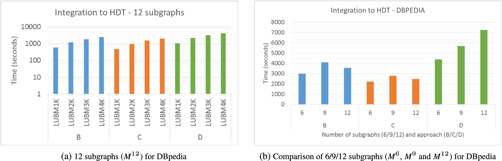
We present the time to integrate the dictionary and triple components of ${\mathit{M}}^{12}$ into the corresponding subgraphs (Fig. 10(a)), for DBpedia. Yet again we see that HDT _crypt-C is the fastest approach, 29% and 56% faster than B and D in DBpedia. In general, all approaches show a linear increase over dataset sizes, as shown in the Appendix.

A comparison in terms of number of subgraphs is shown in Fig. 10(b), reporting the times of merging ${\mathit{M}}^6$ , ${\mathit{M}}^9$ and ${\mathit{M}}^{12}$ for DBpedia (the trends are similar for all datasets). As expected, given that the integration process yields to a partial decompression of the dictionary and triple components, the integration performance follows the same pattern as the decompression. That is, the even distribution of DBpedia results in a faster performance for 6 subgraphs, whereas the excessive duplicates of 12 penalises its performance.

Fig. 11.

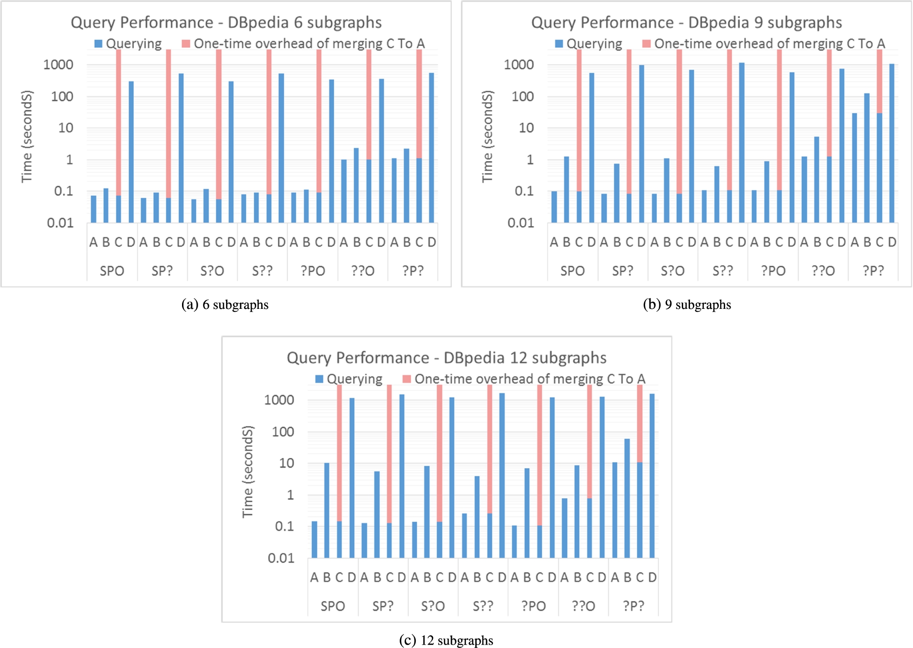
Performance of Triple Patterns over DBpedia (average of the performance in both DBpedia versions).

6.4.2. Query performance

We evaluate the query performance of all partitioning strategies in our use case scenario. Thus, for each subgraph in ${\mathit{M}}^6$ , ${\mathit{M}}^9$ and ${\mathit{M}}^{12}$ (and ${\mathit{M}}_{\mathit{S}}^8$ and ${\mathit{M}}_{\mathit{L}}^8$ in SAFE) we first generate 30 random queries for each triple pattern type,18

¹⁸

All queries are available at the HDTcrypt repository.

assuring an even presence of different predicates. Figure 11 shows the average execution time of the selected queries for both DBpedia versions (the results for LUBM4K and SAFE are presented in the Appendix). Note that, as shown in the previous section, the integration into a new HDT results in a non-negligible time to perform the process. Thus, for HDT _crypt-A , HDT _crypt-B and HDT _crypt-D we follow the strategy where queries are executed locally in each dictionary and triple component. In contrast, query execution in HDT _crypt-C would require the D-union of all the dictionaries to be created, which is then equivalent to integrating HDT _crypt-C into a new HDT to be queried. As such, the performance time for HDT _crypt-C is presented as the sum of the time taken to create one integrated HDT (performed once), as previously explained in Section 6.4.1, and to subsequently query the integrated HDT (note again that this latter is equivalent to querying HDT _crypt-A ).

Regarding the comparison between our strategies for partitioning, results show that HDT _crypt-A and HDT _crypt-B have the best performance for all patterns. This can be attributed to the fact that they benefit from efficient Bitmap Triples indexes, while HDT _crypt-D must use Plain Triples (as stated in Section 5.4) that perform sequential scans to resolve queries. Note that HDT _crypt-D is only competitive in the case of (?p?) queries (i.e. retrieving all subjects and objects related to a given predicate), given that most of the triples are returned and the total time is similar to a full sequential scan. In addition, Bitmap Triples indexes are less efficient for such query types [25]. As previously stated, HDT _crypt-C behaves as HDT _crypt-A but there is a once-off overhead associated with merging all dictionary and triple components into one HDT (represented in red in Fig. 14).

In turn, it is also worth mentioning that HDT _crypt-B query performance is closer to the baseline HDT _crypt-A in the scenario with 6 subgraphs. This is mainly due to the larger number of dictionaries/triples to be queried in a scenario with a higher number of subgraphs (as shown in Table 4), which penalises the HDT _crypt-B and HDT _crypt-D methods. In this scenario, HDT _crypt-A is the most efficient approach for query execution. The noticeable performance difference against the rest of the partitioning approaches suggests that the once-off merging that is required for HDT _crypt-C can be amortised if the dataset is meant for intensive querying after decryption.

Table 7

Summary of performance of different ${\mathrm{HDT}}_{\mathit{crypt}}$ strategies, where ⋆ ⋆ ⋆ stands for the best performance

Strategy	Comp. & encryp.			Decryp. & decomp.	Querying
	Time	Size	Preconditions	Time	Time	Preconditions
crypt-A	⋆ ⋆	⋆	None	⋆	⋆ ⋆ ⋆	None
crypt-B	⋆	⋆ ⋆	HDT of full graph G	⋆ ⋆	⋆ ⋆	None
crypt-C	⋆ ⋆ ⋆	⋆ ⋆ ⋆	HDT of full graph G	⋆ ⋆ ⋆	⋆ ⋆	Once-off integration to a new HDT
crypt-D	⋆	⋆ ⋆ ⋆	HDT of full graph G	⋆ ⋆	⋆	None

Table 8

Influence of the increasing number of subgraphs and duplicates in the performance of different ${\mathrm{HDT}}_{\mathit{crypt}}$ strategies, where $+++$ stands for very positive and $---$ for very negative

Strategy	Comp. & encryp.		Decryp. & decomp.	Querying
	Time	Size	Time	Time
crypt-A	−	−	−	−
crypt-B	−	$+++$	−	−
crypt-C	−	$+++$	−	−
crypt-D	$---$	$++$	−	$--$

6.5. Discussion of the results

Overall, our empirical evaluation showed interesting results and allows us to draw conclusions on the applicability of each strategy. We summarize a ranking of results for each scenario in Table 7, and we outline the influence of the increasing number of subgraphs and duplicates in the data in Table 8, detailed as follows:

• HDT _crypt-C is the most effective technique in terms of compression and decompression times, as well as compression sizes. In particular, it achieves additional 26–33% space saving over the –already compressed – baseline (HDT _crypt-A ), and it is 37–40% faster to compress, and 30% faster to decompress. Note that the impact of these space and time savings are even more noticeable when dealing with big data. As we noticed, if the original HDT of the full graph is not available beforehand, then the creation of HDT _crypt-C can take more time than the baseline (it results in approx. the same time in LUBM and 35–50% slower in DBpedia, with a rich dictionary of terms), but it keeps the aforementioned noticeable space savings. In the extreme case of isolated subgraphs with few duplicates, as in SAFE, HDT _crypt-C takes the same space as the baseline and is still 18% faster to encrypt.

• In contrast, HDT _crypt-C does not allow the user to directly query the exchanged information. If such a scenario is required, this can be solved with a once-off conversion from HDT _crypt-C to HDT _crypt-A . This conversion can be done for any strategy, but it is indeed faster for HDT _crypt-C .

• HDT _crypt-B and HDT _crypt-D also reduce the size of the baseline (HDT _crypt-A ), and can be directly queried. Results show that HDT _crypt-B and HDT _crypt-D gain 6–24% and 24–26% space over the baseline respectively, at the cost of an extra 68% and 23% time for compression (performed only once by the data publisher). In turn, the decompression time outperforms the baseline by 7% and 9% for HDT _crypt-B and HDT _crypt-D respectively. In the extreme case of isolated subgraphs with few duplicates, as in SAFE, HDT _crypt-B and HDT _crypt-D suffer from a slight space overhead (15–23%) over the baseline, and non negligible additional decompressing times.

• The performance of directly querying several subgraphs in HDT _crypt-B is close to the baseline HDT _crypt-A . Nonetheless, it is penalised at larger number of partitions (such as 12 in our experiments) and larger number of duplicates (such as our even distribution in DBpedia). HDT _crypt-D suffers from the additional problem of performing sequential scans, and is not competitive but for queries that retrieve large number of results.

• Encryption and decryption times are almost negligible compared to the compression/decompression counterparts.

• Compression sizes, compression and decompression times show linear growth with increasing dataset size.

• In general, an increasing number of subgraphs leads to more duplicates and more space savings of our novel HDT _crypt-B , HDT _crypt-C and HDT _crypt-D partitioning approaches over the baseline HDT _crypt-A . In turn, less data file sizes result in faster decompression of our novel approaches. In contrast, the compression time is penalised given that more components have to be generated. Our experiments also showed that the number of subgraphs does not have a strong influence on the query performance, but the skewed distribution of sizes and the large number of components (such as in DBpedia) can result in slight differences between scenarios.

Fig. 12.

Integration of the dictionary and triple components of ${\mathit{M}}^6$ , ${\mathit{M}}^9$ and ${\mathit{M}}^{12}$ into one HDT per subgraph.

7. Conclusions and future work

To date Linked Data publishers have focused on exposing and linking open data, however the Linked Data infrastructure could be extended to cater for the storage and exchange of confidential data. In this paper, we discussed how HDT compression can be extended to cater for RDF datasets which needs to be encrypted. Specifically, we proposed a number of different compression strategies that are compatible and demonstrated the need for careful integration when it comes to compressed encrypted RDF data. From our evaluation we can see that our proposal HDT _crypt-C outperforms the other partitioning strategies both in terms of compression and decompression time, and it also produces the most compact representation, resulting in 26–31% space savings over the – already compressed – baseline. HDT _crypt-B and HDT _crypt-D also reduce the size of the baseline significantly. Whereas, when it comes to querying HDT _crypt-A and HDT _crypt-B outperform HDT _crypt-C , which incurs additional overhead as the dictionaries and triples need to be integrated in order to support querying. Additionally, we note that compression, decompression and query performance is influenced both by the number of access restricted subgraphs and the distribution of triples across subgraphs, especially in HDT _crypt-D . In future work, we plan to extend our existing work to cater for querying over encrypted compressed data without the need for decryption. Our current work considers basic triple pattern resolution, while the HDT approach can be used as the basic engine to resolve full SPARQL queries. Our plan is to support this possibility on the compressed and encrypted data in future work.