Effective and efficient Semantic Table Interpretation using TableMiner +

Abstract

This article introduces TableMiner⁺, a Semantic Table Interpretation method that annotates Web tables in a both effective and efficient way. Built on our previous work TableMiner, the extended version advances state-of-the-art in several ways. First, it improves annotation accuracy by making innovative use of various types of contextual information both inside and outside tables as features for inference. Second, it reduces computational overheads by adopting an incremental, bootstrapping approach that starts by creating preliminary and partial annotations of a table using ‘sample’ data in the table, then using the outcome as ‘seed’ to guide interpretation of remaining contents. This is then followed by a message passing process that iteratively refines results on the entire table to create the final optimal annotations. Third, it is able to handle all annotation tasks of Semantic Table Interpretation (e.g., annotating a column, or entity cells) while state-of-the-art methods are limited in different ways. We also compile the largest dataset known to date and extensively evaluate TableMiner⁺ against four baselines and two re-implemented (near-identical, as adaptations are needed due to the use of different knowledge bases) state-of-the-art methods. TableMiner⁺ consistently outperforms all models under all experimental settings. On the two most diverse datasets covering multiple domains and various table schemata, it achieves improvement in F1 by between 1 and 42 percentage points depending on specific annotation tasks. It also significantly reduces computational overheads in terms of wall-clock time when compared against classic methods that ‘exhaustively’ process the entire table content to build features for inference. As a concrete example, compared against a method based on joint inference implemented with parallel computation, the non-parallel implementation of TableMiner⁺ achieves significant improvement in learning accuracy and almost orders of magnitude of savings in wall-clock time.

1. Introduction

Recovering semantics from tables is a crucial task in realizing the vision of the Semantic Web. On the one hand, the amount of high-quality tables containing useful relational data is growing rapidly to hundreds of millions [3,4]. On the other hand, search engines typically ignore underlying semantics of such structures at indexing, hence performing poorly on tabular data [21,24]. Research directed to this particular problem is Semantic Table Interpretation [2,7,14,15,21,23–26,35,36], which deals with three types of annotation tasks in tables. Starting with the input of a well-formed relational table (e.g., Fig. 1), and reference sets of concepts (or classes, types), named entities (or simply ‘entities’) and relations, semantic table interpretation aims to: (1) link entity mentions in content cells (or simply ‘cells’) to the reference entities (disambiguation); (2) annotate columns with semantic concepts if they contain entity mentions (NE-columns), or properties of concepts if they contain data literals (literal-columns); and (3) identify the semantic relations between columns. The annotations created can enable semantic indexing and search of the data and used to create Linked Open Data (LOD).

Fig. 1.

An example Wikipedia webpage containing a relational table (Last retrieved on 9 April 2014).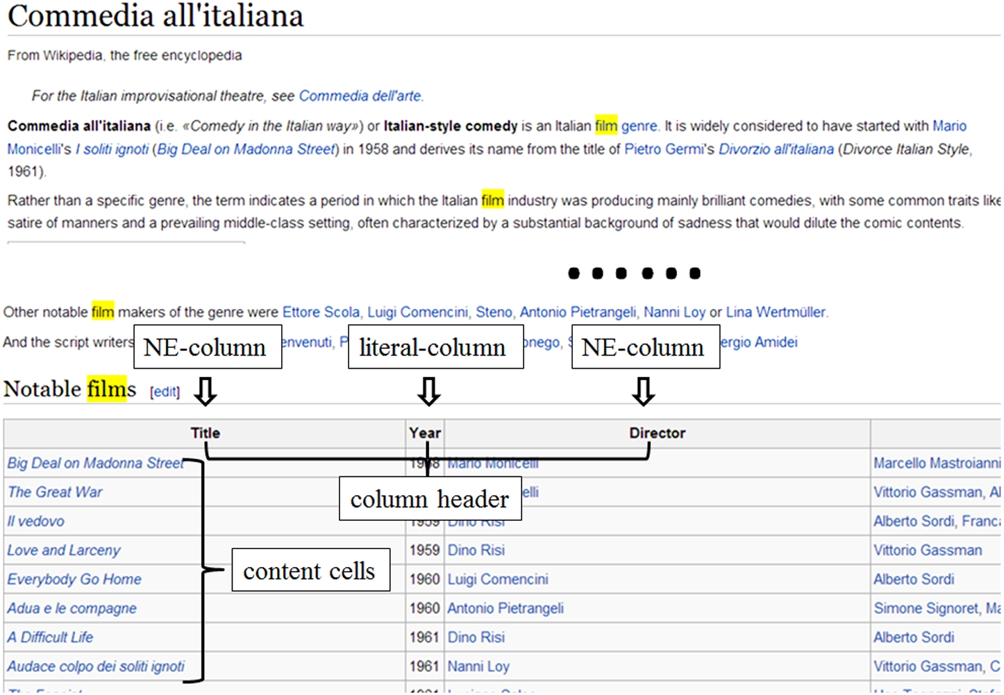

Although classic Natural Language Processing (NLP) and Information Extraction (IE) techniques address similar research problems [5,10,28,45], they are tailored for well-formed sentences in unstructured texts, and are unlikely to succeed on tabular data [21,24]. Typical Semantic Table Interpretation methods make extensive use of structured knowledge bases, which contain candidate concepts and entities, each defined with rich lexical and semantic information and linked by relations. The general workflow involves: (1) retrieving candidates corresponding to table components (e.g., concepts given a column header, or entities given the text of a cell) from the knowledge base, (2) represent candidates using features extracted from both the knowledge base and tables to model semantic interdependence between table components and candidates (e.g., the header text of a column and the name of a candidate concept), and between various table components (e.g., a column should be annotated by a concept that is shared by all entities in the cells from the column), and (3) applying inference to choose the best candidates.

This work addresses several limitations of state-of-the-art on three dimensions: effectiveness, efficiency, and completeness.

Effectiveness – Semantic Table Interpretation methods so far have primarily exploited features derived from two sources: the knowledge bases, and table components such as header and row content (to be called ‘in-table context’). In this work, we propose to utilize the so-called ‘out-table context’, i.e., the textual content around and outside tables (e.g., paragraphs, captions), to further improve interpretation accuracy. As an example, the first column in the table shown in Fig. 1 (to be called the ‘example table’) has a header ‘Title’, which is highly ambiguous and arguably irrelevant to the concept we should use to annotate the column. However, on the containing webpage, the word ‘film’ is repeated 17 times. This is a strong indicator for us to select a suitable concept for the column. A particular type of out-table context we utilize is the semantic markups inserted within webpages by data publishers such as RDFa/Microdata annotations. These markups are growing rapidly as major search engines use them to enable semantic indexing and search. When available, they provide high-quality, important information about the webpages and tables they contain.

We show empirically that we can derive useful features from out-table context to improve annotation accuracy. Such out-table features are highly generic and generally available. While on the contrary, many existing methods use knowledge base specific features that are impossible to generalize, or suffer substantially in terms of accuracy when they can be adapted, which we shall show in experiments.

Efficiency – We argue that efficiency is also an important factor to consider in the task of Semantic Table Interpretation, even though it has never been explicitly addressed before. The major bottleneck is mainly due to three types of operations: querying the knowledge bases, building feature representations for candidates, and computing similarity between candidates. Both the number of queries and similarity computation can grow quadratically with respect to the size of a table as often such operations are required for each pair of candidates [21,24,27]. Empirically, Limaye et al. [21] show that the actual inference algorithm only consumes less than 1% of total running time. Using a local copy of the knowledge base only partially addresses the issue but introduces more problems. First, hosting a local knowledge base requires infrastructural support and involves set-up and maintenance. As we enter the ‘Big-Data’ era, knowledge bases are growing rapidly towards a colossal structure such as the Google Knowledge Graph [33], which constantly integrates increasing numbers of heterogeneous sources. Maintaining a local copy of such a knowledge base is likely to require an infrastructure that not every organization can afford [29]. Second, local data are not guaranteed to be up-to-date. Third, scaling up to very large amount of input data requires efficient algorithms in addition to parallelization [32], as the process could be bound by the large number of I/O operations. Therefore in our view, a more versatile solution is cutting down the number of queries and data items to be processed. This reduces I/O operations in both local and remote scenarios, also reducing costs associated with making remote calls to Web service providers.

In this direction, we identify an opportunity to improve state-of-the-art in terms of efficiency. To illustrate, consider the example table that in reality contains over 60 rows. To annotate each column, existing methods would use content from every row in the column. However, from a human reader’s point of view, this is unnecessary. Simply reading the eight rows one can confidently assign a concept to the column to best describe its content. Being able to make such inference with limited data would give substantial efficiency advantage to Semantic Table Interpretation algorithms, as it will significantly reduce the number of queries to the underlying knowledge bases and the number of candidates to be considered for inference.

Completeness – Many existing methods only deal with one or two types of annotation tasks in a table [35,36]. In those that deal with all tasks [7,21,23–25], only NE-columns are considered. As shown in Fig. 1, tables can contain both NE-columns containing entity mentions, and literal-columns containing data values of entities on the corresponding rows. Methods such as Limaye et al. [21] and Mulwad et al. [24] can recognize relations between the first and third columns, but are unable to identify the relation between the first and the second columns. We argue that a Semantic Table Interpretation method should be able to annotate both NE-columns and literal-columns.

To address these issues, we developed TableMiner previously [42] that uses features from both in- and out-table context and annotates NE-columns and cells in a relational table based on the principle of ‘start small, build complete’. That is, (1) create preliminary, likely erroneous annotations based on partial table content and a simple model assuming limited interdependence between table components; (2) and then iteratively optimize the preliminary annotations by enforcing interdependence between table components. In this work we extend it to build TableMiner⁺, by adding ‘subject column’ [35,36] detection, relation enumeration, and improving the iterative optimization process. Concretely, TableMiner⁺ firstly interprets NE-columns (to be called column interpretation), while coupling column classification and entity disambiguation in a mutually recursive process that consists of a LEARNING phase and an UPDATE phase. The LEARNING phase interprets each column independently by firstly learning to create preliminary column annotations using an automatically determined ‘sample’ from the column, followed by ‘constrained’ entity disambiguation of the cells in the column (limiting candidate entity space using preliminary column annotations). The UPDATE phase iteratively optimizes the classification and disambiguation results in each column based on a notion of ‘domain consensus’ that captures inter-column and inter-task dependence, creating a global optimum. For relation enumeration, TableMiner⁺ detects a subject column in a table and infers its relations with other columns (both NE- and literal-columns) in the table.

TableMiner⁺ is evaluated on four datasets containing over 15,000 tables, against four baselines and two re-implemented near-identical1 ¹

Despite our best effort, identical replication of existing systems and experiments has been not possible due to many reasons, see Appendix D.

state-of-the-art methods. It consistently obtains the best performance on all datasets. On the two most diverse datasets covering multiple domains and various table schemata, it obtains an improvement of about 1–18 percentage points in disambiguation, 6–42 in classification, and 4–16 in relation enumeration. It is also very efficient, contributing up to 66% reduction in terms of the amount of candidates to be processed and up to 29% savings in wall-clock time compared against exhaustive baseline methods. Even in the setting where a local copy of the knowledge base is used, TableMiner⁺ delivers almost orders of magnitude savings in wall-clock time compared against one re-implemented state-of-the-art method.

The remainder of this paper is organized as follows. Section 2 defines terms and concepts used in the relevant domain. Section 3 discusses related work. Sections 4 to 9 introduce TableMiner⁺ in detail. Sections 10 and 11 describe experiment settings and discuss results, followed by conclusion in Section 12.

2. Terms and concepts

A relational table contains regular rows and columns resembling tables in traditional databases. In practice, Web tables containing complex structures constitute a small population and have not been the focus of research. In theory, complex tables can be interpreted by adding a pre-process that parse complex structures using methods such as Zanibbi et al. [39].

Relational tables may or may not contain a header row, which is typically the first row in a table. They often contain a subject column that usually (but not necessarily) corresponds to the ‘primary key’ columns in a database table [35,36]. This contains the set of entities the table is about (subject entities, e.g., column ‘Title’ in Fig. 1 contains a list of films the table is about), while other columns contain either entities forming binary relationships with subject entities, or literals describing attributes of subject entities.

A knowledge base defines a set of concepts (or types, classes), their object instances or entities, literals representing concrete data values, and semantic relations that define possible associations between entities (hence also between concepts they belong to), or between an entity and a literal, in which case the relation is usually called a property of the entity (hence a property of its concept) and the literal as the property value. In the generic form, a knowledge base is a liked data set containing a set of triples, statements, or facts, each composed of a subject, predicate and object. The subject could be a concept or entity, the object could be a concept, entity, or literal, and the predicate could be a relation or property. A knowledge base can be a populated ontology, such as the YAGO2

²

http://www.mpi-inf.mpg.de/yago-naga/yago/.

and DBpedia3 ³

http://wiki.dbpedia.org/Ontology.

datasets, in which case a concept hierarchy is defined. However this is not always true as some knowledge bases do not define strict ontology but loose concept networks, such as Freebase.4 ⁴

http://www.freebase.com.

The task of Semantic Table Interpretation addresses three annotation tasks. Named Entity Disambiguation associates each cell in NE-columns with one canonical entity; column classification annotates each NE-column with one concept, or in the case of literal-columns, associates the column to one property of the concept assigned to the subject column of the table; Relation Extraction (or enumeration) identifies binary relations between NE-columns, or in the case of one NE-column and a literal-column and given that the NE-column is annotated by a specific concept, identifies a property of that concept that could explain the data literals. The candidate entities, concepts and relations are drawn from the knowledge base.

Using the example table and Freebase as example, the first column can be considered a reasonable subject column and should be annotated by the Freebase type ‘Film’ (URI ‘fb:5 ⁵

fb:http://www.freebase.com.

/film/film’). ‘A Difficult Life’ in the first column should be annotated by ‘fb:/m/02qlhz2’ that denotes a movie directed by ‘Dino Risi’ (in the third column, ‘fb:/m/0j_nhj’). The relation between the first and third column should be annotated as ‘Directed by’ (‘fb:/film/film/directed_by’). And the relation between the first and second column (which is a literal-column) should be the property of ‘Film’: ‘initial release date’ (‘fb:/film/film/initial_release_date’), which we also use to annotate the second column.

3. Related work

3.1. Legacy tabular data to linked data

Research on converting tabular data in legacy data sources to linked data format has made solid contribution toward the rapid growth of the LOD cloud in the past decade [6,12,19,30]. The key difference from the task of Semantic Table Interpretation is that the focus is on data generation rather than interpretation, since the goal is to pragmatically convert tabular data from databases, spreadsheets, and similar data structures into RDF. Typical methods require manually (or partially automated) mapping the two data structures (input and output RDF), and they do not link data to existing concepts, entities and relations from the LOD cloud. As a result, the implicit semantics of the data remain uncovered.

3.2. General NLP and IE

Some may argue to use the general purpose NLP/IE methods for Semantic Table Interpretation, due to their highly similar objectives. This is infeasible for a number of reasons. First, state-of-the-art methods [17,31] are typically tailored to unstructured text content that is different from tabular data. The interdependence among the table components cannot be easily modeled in such methods [22]. Second and particularly for the tasks of Named Entity Classification and Relation Extraction, classic methods require each target semantic label (i.e., concept or relation) to be pre-defined and learning requires training or seed data [28,40]. In Semantic Table Interpretation however, due to the large degree of variations in table schemata (e.g., Limaye et al. [21] use a dataset of over 6,000 randomly crawled Web tables of which no information about the table schemata is known a priori), defining a comprehensive set of semantic concepts and relations and subsequently creating necessary training or seed data are infeasible.

A related IE task tailored to structured data is wrapper induction [9,18], which automatically learns wrappers that can extract information from regular, recurrent structures (e.g., product attributes from Amazon webpages). In the context of relational tables, wrapper induction methods can be adapted to annotate table columns that describe entity attributes. However, they also require training data and the table schemata to be known a priori.

3.3. Table extension and augmentation

Table extension and augmentation aims at gathering relational tables that contain the same entities but cover complementary attributes of the entities, and integrate these tables by joining them on the same entities. For example, Yakout et al. [38] propose InfoGather for populating a table of entities with their attributes by harvesting related tables on the Web. The users need to either provide the desired attribute names of the entities, or example values of their attributes. The system can also discover the set of attributes for similar entities. Bhagavatula et al. [1] introduce WikiTables, which given a query table and a collection of other tables, identifies columns from other tables that would make relevant additions to the query table. They first identify a reference column (e.g., country names in a table of country population) in the query table to use for joining, then find a different table (e.g. a list of countries by GDP) with a column similar to the reference column, and perform a left outer join to augment the query table with an automatically selected column from the new table (e.g., the GDP amounts). Lehmberg et al. [20] create the Mannheim Search Joins Engine with the same goal as WikiTables but focus on handling tens of millions of tables from heterogeneous sources.

The key difference between these systems and the task of Semantic Table Interpretation is that they focus on integration rather than interpretation. The data collected are not linked to knowledge bases and ambiguity still remains.

3.4. Semantic Table Interpretation

Hignette et al. [14,15] and Buche et al. [2] propose methods to identify concepts represented by table columns and detect relations present in tables in a domain-specific context. An NE-column is annotated based on two factors: similarity between the header text of the column and the name of a candidate concept; plus the similarities calculated for each cell in the column and each term in the hierarchical paths containing the candidate concept. For relations, they only detect the presence of semantic relations in the table without specifying the columns that form binary relations.

Venetis et al. [35] annotate table columns and identify relations between the subject column and other columns using types and relations from a database constructed by mining the Web using lexico-syntactic patterns such as the Hearst patterns [13]. The database contains co-occurrence statistics about the subject and object of triples, such as the number of times the word ‘cat’ and ‘animal’ extracted by the pattern $⟨?\mathrm{,}\mathit{such}\mathit{as}\mathrm{,}?⟩$ representing the is-a relation between concept and instances. A maximum likelihood inference model predicts the best type for a column to be the one maximizing the probability of seeing all the values in the column given that type for the column. Such probability is computed based on the co-occurrence statistics gathered in the database. Relation interpretation follows the same principle.

Likewise, Wang et al. [36] argue that tables describe a single entity type (concept) and its attributes and therefore, consist of an entity column (subject column) and multiple attribute columns. The goal is to firstly identify the entity column in the table, then associate a concept from the Probase knowledge base [37] that best describes the table schema. Essentially this allows annotating the subject NE-column and literal-columns using properties of the concept, also identifying relations between the subject column and other columns. Probase is a probabilistic database built in the similar way as that in Venetis et al. [35] and contains an inverted index that supports searching and ranking candidate concepts given a list of terms describing possible concept properties, or names describing possible instances. The method heavily depends on these features and the probability statistics gathered in the database.

Muñoz et al. [26] extract RDF triples for relational tables from Wikipedia articles. The cells in the tables must have internal links to other Wikipedia articles. These are firstly mapped to DBpedia named entities based on the internal links, then to derive relations between two entities on the same row and from different columns, the authors query the DBpedia dataset for triples in the form of $⟨\mathit{subject}\mathrm{,}?\mathrm{,}\mathit{object}⟩$ , where subject and object are replaced by the two mapped entities. Any predicates found in the query result are considered as relations between the two entities. The work is later extended in Muñoz et al. [27] by adding a machine learning process to filter triples that are likely to be incorrect, exploiting features derived from both the knowledge base and the text content from the target cells.

Zwicklbauer et al. [46] use a simple majority vote model for column classification. Each candidate entity in the cells of the column casts a vote to the concept it belongs to, and the one that receives the most votes is the concept used to annotate the column. They show that for this very specific task, it is unnecessary to exhaustively disambiguate each cell in a column. Instead, comparable accuracy can be obtained by using a fraction of the cells from the column. However, the sample size is arbitrarily decided.

Syed et al. [7] deal with all three annotation tasks using DBpedia and Wikitology [34], the latter of which contains an index of Wikipedia articles describing entities and a classification system that integrates several vocabularies including the DBpedia ontology, YAGO, WordNet6

⁶

http://wordnet.princeton.edu/.

and Freebase. The method begins by firstly annotating each NE-column based on candidate entities from every cell in the column. Candidate entities for each cell are retrieved by composing structured queries to match the cell text, the row content, and the column header against different fields defined in the Wikitology index, such as the title and redirects, the first sentence and links from candidate entities’ original Wikipedia articles. Candidate concepts for the column combines the types associated with each candidate entity from each cell, and the scores are based on the number of candidate entities associated with that concept and the relevance score of candidate entities in the search results returned by Wikitology. The column annotations are then used as input in Named Entity Disambiguation, which is cast as queries to Wikitology with new constraints using the column’s annotation. Finally, relations between two NE-columns are derived based on the similar method by Muñoz et al. [26] using DBpedia. This method is later used in Mulwad et al. [25] and Mulwad et al. [23].

Limaye et al. [21] propose to model table components and their interdependence using a probabilistic graphical model. The model consists of two components: ‘variables’ that model different table components, and ‘factors’ that are further divided into node factors modeling the compatibility between the variable and each of its candidate, and edge factors modeling the compatibility between the variables believed to be correlated. For example, given an NE-column, the header of the column is a variable that takes values from a set of candidate concepts; and each cell in the column is a variable that takes values from a set of candidate entities. The node factor for the header could model the compatibility between the header text and the names of each candidate concept; while the edge factor could model the compatibility between any candidate concept for the header and any candidate entity from each cell. The strength of compatibility could be measured using methods such as string similarity metrics [11] and semantic similarity measures [43]. Then the task of inference amounts to searching for an assignment of values to the variables that maximizes the joint probability. A unique feature of this method is that it solves the three annotation tasks simultaneously, capturing interdependence between various table components at inference, while other methods either tackle individual annotation tasks or tackles each separately and sequentially.

Mulwad et al. [24] argue that computing the joint probability distribution in Limaye’s method is very expensive. Built on the earlier work by Syed et al. [7] and Mulwad et al. [23,25], they propose a light-weight semantic message passing algorithm that applies inference to the same kind of graphical model. This is similar to TableMiner⁺ in the way that the UPDATE phase of TableMiner⁺ can be considered as a similar semantic message passing process. However, TableMiner⁺ is fundamentally different since it (1) adds a subject column detection algorithm; (2) deals with both NE-columns and literal-columns, while Mulwad et al. only handle NE-columns; (3) uses an efficient approach bootstrapped by sampled data from the table while Mulwad et al. build a model that approaches the task in an exhaustive way; (4) defines and uses context around tables as features while Mulwad et al. has used knowledge base specific features; (5) uses different methods for scoring and ranking candidate entities, concepts and relations; and (6) models interdependence differently which, if transforms to an equivalent graphical model, would result in fewer factor nodes.

3.5. Remark

Existing Semantic Table Interpretation methods have several limitations. First, they have not considered using features from out-table context, which is highly generic and generally available. Instead, many have used knowledge base specific features that are difficult or impossible to generalize. For example, the co-occurrence statistics used by Venetis et al. [35] and Wang et al. [36] are unavailable in knowledge bases such as YAGO, DBpedia, and Freebase. Methods such as Limaye et al. [21] and Mulwad et al. [24] use the concept hierarchy in their knowledge bases. However, Freebase does not have a strict concept hierarchy. These methods can become less effective when adapted to different knowledge bases, as we shall show later.

Second, no existing methods explicitly address efficiency, which we argue as an important factor in Semantic Table Interpretation tasks. Current methods are non-efficient because they typically adopt an exhaustive strategy that examines the entire table content, e.g., column classification depends on every cell in the column. This results in quadratic growth of the number of computations and knowledge base queries with respect to the size of tables, as such operations are usually required for every pair of candidates, e.g., candidate relation lookup between every pair of entities on the same row [24,26,27], or similarity computation between every pair of candidate entity and concept in a column [21]. This can be redundant as Zwicklbauer et al. [46] have empirically shown that comparable accuracy can be obtained by using only a fraction of data (i.e., sample) from the column. However, there remains the challenge to automatically determine the optimal sample size and elements.

Further, existing methods are incomplete, since they either only tackle certain annotation tasks [35,36], or only deal with NE-columns [7,21,23–25].

In an attempt to address some of the above issues, we previously developed a prototype TableMiner [42] that is able to annotate NE-columns and disambiguate entity cells in an incremental, mutually recursive and bootstrapping approach seeded by automatically selected sample from a table. And in Zhang [41] we further explored different methods for selecting the sample and its effect on accuracy. This work joins the two and largely extends them in a number ways: (1) adding a new algorithm for subject column detection and for relation enumeration; (2) revising the column classification and entity disambiguation processes (primarily in the UPDATE process); (3) performing significantly more comprehensive experiments to thoroughly evaluate the new method; and (4) releasing both the dataset and software to encourage future research.

4. Overview

Figure 2 shows the data flow and processes of TableMiner⁺. Given a relational table it firstly detects a subject column (Section 6), which is used by later processes of column interpretation and relation enumeration. Then TableMiner⁺ performs NE-column interpretation, coupling column classification with entity disambiguation in an incremental, mutually recursive, bootstrapping approach. This starts with a LEARNING phase (Section 7) that interprets one NE-column at a time independently to create preliminary concept annotation for an NE-column and entity annotation for the cells, followed by an UPDATE phase (Section 8) that iteratively revises the annotations by enforcing interdependence between columns, and between the classification and disambiguation results.

Fig. 2.

The overview of TableMiner⁺. (a) a high-level architecture diagram; (b) detailed architecture with input/output. d – table data. Grey colour indicates annotated table elements. Angle brackets indicates annotations. Inside a table: H – header. E, a, b, x, z – content cells.

In the LEARNING phase, for preliminary column classification (Section 7.2), TableMiner⁺ works in an incremental, iterative manner to gather evidence from each cell in the column at a time until it reaches a stopping criteria (automatically determined), usually before covering all cells in the column. Therefore, TableMiner⁺ can use only partial content in the column to perform column classification. We say that it uses a ‘sample’ from the column for the task and each element in the sample is a cell which TableMiner⁺ has used as evidence for preliminary column classification until stop. In theory, the size and elements of the sample can affect the outcome and hence the accuracy of classification. For this reason, a sample ranking process (Section 7.1) precedes preliminary column classification to re-order table rows based on the cells in the target column with a goal to optimize the sample to obtain the highest accuracy of classification. Next, the preliminary concept annotation for the column is used to constrain entity candidate space in disambiguating cells in the column (preliminary cell disambiguation, Section 7.3). Using a sample for column classification and constraining entity candidate space allows TableMiner⁺ to be more efficient than state-of-the-art methods that exhaustively process all content from a column.

The UPDATE phase begins by taking the entity annotations in all NE-cells to create a ‘domain representation’ (Section 8.1), which is compared against candidate concepts for each NE-column to revise the preliminary column classification results (Section 8.2). If any NE-column’s annotation changes due to this process, the newly elected concept is then used to revise disambiguation results in that column (Section 8.3). This process repeats until no changes are required.

Finally relation enumeration (Section 9) discovers binary relations between the subject column and other NE-columns; or identifies a property of the concept used to annotate the subject column to best describe data in the literal-columns. In the latter case, the property is considered both the annotation for the literal-column, and the relation between the subject column and the literal-column.

The incremental, iterative process used by preliminary column classification is implemented as a generic incremental inference with stopping algorithm (I-Inf), which is also used for subject column detection and is described in Section 5.

At different steps, TableMiner⁺ uses features from both in-table and out-table context listed in Table 1. In particular, out-table context includes table captions, webpage title, surrounding paragraphs, semantic markups inserted within webpages if any. Table captions and the title of the webpage may mention key terms that are likely to be the focus concept in a table. Paragraphs surrounding tables may describe the content in the table, thus containing indicative words of the concepts, relations, or entities in the table. Semantic markups use certain vocabularies (e.g., schema.org) to annotate important pieces of information on a webpage. For example, Fig. 3 shows an annotation on the IMDB webpage of the movie ‘The Godfather (1972)’. Here it annotates the name of the director for the movie. Intuitively if we use this name as contextual features to disambiguate names in the table of cast members on this webpage, we may want to give it a higher weight than other features not included in such semantic markups.

Table 1

Types of context from which features are created for Semantic Table Interpretation

In-table context	Out-table context
column header	webpage title
row content	table caption and/or title
column content	paragraphs (unstructured text)
	semantic markups

Fig. 3.

Example semantic markup in a webpage.

In the following sections we describe details of each component, and we will highlight the changes or additions to the previous TableMiner (if any) in each section. In Appendix F we list an index of mathematical notations and equations that are used throughout the remainder of this article. Readers may use this for quick access to their definitions.

5. I-Inf

We firstly describe the I-Inf algorithm that we have previously introduced in [42]. Here we generalize it so it can be used by both subject column detection and preliminary column classification. As shown in Algorithm 1, it starts by taking input a dataset D, an empty set of key-value pairs $⟨\mathit{k}\mathrm{,}\mathit{v}⟩$ denoting the state, and i indicates the current iteration number. Then it iteratively processes each single data item d from D (function process) to generate a set of key-value pairs, which are used to update the state (function update) by either resetting scores of existing key-value pairs or adding new pairs. At the end of each iteration, I-Inf checks for convergence (function convergence), in which case the algorithm stops. To do so, it computes entropy of the current and previous iterations using the corresponding sets of key-value pairs (Eq. (1)), and convergence happens if the difference between the two entropy values is less than a threshold. $$\begin{array}{}\text{(1)}& \hfill \mathit{entropy}\mathrm{(}\mathit{i}\mathrm{)}& =-{\displaystyle \sum }_{⟨\mathit{k}\mathrm{,}\mathit{v}⟩\in {\{⟨\mathit{k}\mathrm{,}\mathit{v}⟩\}}_{\mathit{i}}}\mathit{P}\mathrm{(}⟨\mathit{k}\mathrm{,}\mathit{v}⟩\mathrm{)}{log}_2\mathit{P}\mathrm{(}⟨\mathit{k}\mathrm{,}\mathit{v}⟩\mathrm{)}\text{(2)}& \hfill \mathit{P}\mathrm{(}⟨\mathit{k}\mathrm{,}\mathit{v}⟩\mathrm{)}& ={\displaystyle \frac{\mathit{v}}{{\sum }_{⟨\mathit{k}\mathrm{,}\mathit{v}⟩\in {\{⟨\mathit{k}\mathrm{,}\mathit{v}⟩\}}_{\mathit{i}}}\mathit{v}}}\end{array}$$ where i indicates the ith iteration. Intuitively, when the entropy converges, we expect $\mathit{P}\mathrm{(}⟨\mathit{k}\mathrm{,}\mathit{v}⟩\mathrm{)}$ for each key-value pair to also converge. This could suggest that the processing of additional data items changes little the value of each key-value pair with respect to the sum for all pairs (i.e., the denominator in Eq. (2)). Effectively this means that although the absolute value for each pair still changes upon additional data items, the change in their relative values may be neglectable and hence their rankings are stabilized. I-Inf will be discussed in more details later where they are used in specific cases.

Algorithm 1

I-inf

6. Subject column detection

6.1. Preprocessing

Subject column detection begins by classifying cells from each column (denoted by ${\mathit{T}}_{\mathit{j}}$ ) into one of the data types: ‘empty’, ‘named entity’, ‘number’, ‘date expression’, ‘long text’ (e.g., sentence, or paragraph), and ‘other’. This is done by using simple regular expressions that examine the syntactic features of cell text, such as number of words, capitalization, mentions of months or days in a week. A vast amount of literature can be found on this topic [2,14,15]. Then each column is assigned a most frequent datatype by counting the number of cells belonging to that type. The only exception is that a column is empty only if all cells are empty.

Next, if a candidate NE-column has a column header that is a preposition word, it is discarded. An example like this is shown in Fig. 4, where the columns ‘For’ and ‘Against’ are clearly not subject columns but rather form relations with the subject column ‘Batsman’.

Fig. 4.

An example table containing columns with preposition words as headers.

6.2. Features

Next, features listed in Table 2 are constructed for each remaining candidate NE-column. The fraction of empty cells (emc) of a column is simply the number of empty cells divided by the number of rows in the column. Likewise, the fraction of cells with unique content (uc) is a ratio between the number of cells with unique text content and the number of rows. The distance from the first NE-column (df) counts how many columns the current column is away from the first candidate NE-column from the left. NE-columns are also checked by regular expressions to identify the number of cells likely to contain acronyms or ids such as airline IACO codes (e.g., using features like uppercase letters and presence of white spaces). A column that is an acronym or id column ( $\mathit{ac}\mathrm{(}{\mathit{T}}_{\mathit{j}}\mathrm{)}=1$ , or 0 otherwise) is disfavored. The intuition is that as the subject of a table one would prefer to use full names of entities for the purpose of clarity.

Table 2

Features used for subject column detection. Examples are based on the visible content in the example table

Feature	Notation	Example
Fraction of empty cells	emc	0.0 for column ‘Title’
Fraction of cells with unique content	uc	1.0 for column ‘Title’, 5/8 for column ‘Director’
If >50% cells contain acronym or id	ac	–
Distance from the first NE-column	df	0 for column ‘Title’, 2 for column ‘Director’
Context match score	cm	–
Web search score	ws	–

Context match score (cm) for a column ${\mathit{T}}_{\mathit{j}}$ counts the frequency of the column header’s composing words in the header’s context: $$\begin{array}{}\text{(3)}& \hfill \mathit{cm}\mathrm{(}{\mathit{T}}_{\mathit{j}}\mathrm{)}={\displaystyle \sum }_{{\mathit{x}}_{\mathit{j}}\in {\mathit{X}}_{\mathit{j}}}{\displaystyle \sum }_{\mathit{w}\in \mathit{bow}\mathrm{(}{\mathit{T}}_{\mathit{j}}\mathrm{)}}\mathit{freq}\mathrm{(}\mathit{w}\mathrm{,}{\mathit{x}}_{\mathit{j}}\mathrm{)}\times \mathit{wt}\mathrm{(}{\mathit{x}}_{\mathit{j}}\mathrm{)}& \end{array}$$ where ${\mathit{x}}_{\mathit{j}}\in {\mathit{X}}_{\mathit{j}}$ are different types of context for the header of column ${\mathit{T}}_{\mathit{j}}$ , $\mathit{bow}\mathrm{(}{\mathit{T}}_{\mathit{j}}\mathrm{)}$ returns the bag-of-words representation of the column header’s text $\mathit{l}\mathrm{(}{\mathit{T}}_{\mathit{j}}\mathrm{)}$ , and $\mathit{wt}\mathrm{(}{\mathit{x}}_{\mathit{j}}\mathrm{)}$ is the weight given to a specific type of context. Intuitively, the more frequent a column header text is repeated in the table’s context the more likely it is the subject column of the table. The context elements used for computing cm include webpage title, table caption and surrounding paragraphs.

Web search score (ws) of a column gathers evidence from the Web to predict the likelihood of it being the subject column, and it is contributed by individual rows in the table. Given a table row ${\mathit{T}}_{\mathit{i}}$ , a query string is firstly created by concatenating all text content from cells on this row, i.e., $\mathit{l}\mathrm{(}{\mathit{T}}_{\mathit{i}\mathrm{,}\mathit{j}}\mathrm{)}$ for all j. Then the query is sent to a search engine to retrieve the top n webpages. Let P denote these webpages, then each NE-cell that composes the query receives a score as: $$\begin{array}{ll}\text{(4)}& \hfill & \mathit{ws}\mathrm{(}{\mathit{T}}_{\mathit{i}\mathrm{,}\mathit{j}}\mathrm{)}=\mathit{countp}\mathrm{(}{\mathit{T}}_{\mathit{i}\mathrm{,}\mathit{j}}\mathrm{,}\mathit{P}\mathrm{)}+\mathit{countw}\mathrm{(}{\mathit{T}}_{\mathit{i}\mathrm{,}\mathit{j}}\mathrm{,}\mathit{P}\mathrm{)}\hfill & \mathit{countp}\mathrm{(}{\mathit{T}}_{\mathit{i}\mathrm{,}\mathit{j}}\mathrm{,}\mathit{P}\mathrm{)}\\ \hfill & ={\displaystyle \sum }_{\mathit{p}\in \mathit{P}}\mathrm{(}\mathit{freq}\mathrm{(}\mathit{l}\mathrm{(}{\mathit{T}}_{\mathit{i}\mathrm{,}\mathit{j}}\mathrm{)}\mathrm{,}{\mathit{p}}_{\mathit{title}}\mathrm{)}\times 2\\ \text{(5)}& \hfill & +\mathit{freq}\mathrm{(}\mathit{l}\mathrm{(}{\mathit{T}}_{\mathit{i}\mathrm{,}\mathit{j}}\mathrm{)}\mathrm{,}{\mathit{p}}_{\mathit{snippet}}\mathrm{)}\mathrm{)}\hfill & \mathit{countw}\mathrm{(}{\mathit{T}}_{\mathit{i}\mathrm{,}\mathit{j}}\mathrm{,}\mathit{P}\mathrm{)}\\ \hfill & ={\displaystyle \sum }_{\mathit{p}\in \mathit{P}}{\displaystyle \sum }_{\mathit{w}\in \mathit{bowset}\mathrm{(}{\mathit{T}}_{\mathit{i}\mathrm{,}\mathit{j}}\mathrm{)}}{\displaystyle \frac{1}{|\mathit{bow}\mathrm{(}{\mathit{T}}_{\mathit{i}\mathrm{,}\mathit{j}}\mathrm{)}|}}\\ \text{(6)}& \hfill & \times \mathrm{(}{\mathit{freq}}^{-}\mathrm{(}\mathit{w}\mathrm{,}{\mathit{p}}_{\mathit{title}}\mathrm{)}\times 2+{\mathit{freq}}^{-}\mathrm{(}\mathit{w}\mathrm{,}{\mathit{p}}_{\mathit{snippet}}\mathrm{)}\mathrm{)}\end{array}$$ $\mathit{countp}$ sums up the frequency of the cell text $\mathit{l}\mathrm{(}{\mathit{T}}_{\mathit{i}\mathrm{,}\mathit{j}}\mathrm{)}$ in both the titles ( ${\mathit{p}}_{\mathit{title}}$ ) and snippets ( ${\mathit{p}}_{\mathit{snippet}}$ ) of returned webpages. Frequency in titles are given double weight as they are considered to be more important. $\mathit{countw}$ firstly transforms cell text into a set of unique words $\mathit{bowset}\mathrm{(}{\mathit{T}}_{\mathit{i}\mathrm{,}\mathit{j}}\mathrm{)}$ , then counts frequency of each word. ${\mathit{freq}}^{-}$ ensures those occurrences of w that are part of occurrences of $\mathit{l}\mathrm{(}{\mathit{T}}_{\mathit{i}\mathrm{,}\mathit{j}}\mathrm{)}$ are eliminated and not double counted. $\mathit{bow}\mathrm{(}{\mathit{T}}_{\mathit{i}\mathrm{,}\mathit{j}}\mathrm{)}$ returns the bag-of-words representation of the cell text.

For each row, the cell that receives the highest score is considered to be containing the subject entity for the row. The intuition is that the query should contain the name of the subject entity plus contextual information of the entity’s attributes. When searched, it is likely to retrieve more documents regarding the subject entity than its attributes, and the subject entity is also expected to be repeated more frequently. Example 1.

For the first content row in the example table, we create a query by concatenating text from the 1st, 3rd and 4th cells on the row (only NE-columns are candidates of subject columns), i.e., ‘big deal on madonna street, mario monicelli, marcello mastroianni’. This is searched on the Web to return a list of documents. Then for each document, we count the frequency of each phrase in the title and snippet and compute countp for each corresponding cell. Next, take the 1st cell for example, ‘big deal on madonna street’ is transformed to a set of unique words {‘big’, ‘deal’, ‘madonna’, ‘street’}, and we count the frequency of each word in the titles and snippets of each document to compute countw. If any occurrence is part of an occurrence of the whole phrase that is already counted in countp, we ignore them. Likewise, we repeat this for the 3rd and 4th cells. Finally, we find that the 1st cell receives the highest Web search score, and we mark it as the subject entity for this row.

In principle the Web search score of a column $\mathit{ws}\mathrm{(}{\mathit{T}}_{\mathit{j}}\mathrm{)}$ simply adds up $\mathit{ws}\mathrm{(}{\mathit{T}}_{\mathit{i}\mathrm{,}\mathit{j}}\mathrm{)}$ for every row i in the column. However, this is practically inefficient and extremely resource consuming as Web search APIs typically has limited quota. In fact, it is also unnecessary. Again using the example table, we do not need to read all 60 rows to decide the column ‘Title’ as the subject column. Therefore, we compute Web search scores of a column in the context of the I-Inf algorithm. To do so, we simply need to define D as the collection of table rows ${\mathit{T}}_{\mathit{i}}$ , and each key-value pair as $⟨{\mathit{T}}_{\mathit{j}}\mathrm{,}\mathit{ws}\mathrm{(}{\mathit{T}}_{\mathit{j}}\mathrm{)}⟩$ .

Example 2.

Following Example 1, we obtain three key-value pairs after processing the first content row: $⟨{\mathit{T}}_1\mathrm{,}10⟩$ , $⟨{\mathit{T}}_3\mathrm{,}5⟩$ and $⟨{\mathit{T}}_4\mathrm{,}2⟩$ , where ${\mathit{T}}_1$ , ${\mathit{T}}_3$ and ${\mathit{T}}_4$ are columns and 10, 5 and 2 are hypothetical Web search scores for the cell ${\mathit{T}}_{1\mathrm{,}1}$ , ${\mathit{T}}_{1\mathrm{,}3}$ , and ${\mathit{T}}_{1\mathrm{,}4}$ respectively. We continue to process the remaining rows one at a time by repeating the process, each time updating the set of key-value pairs with the Web search scores obtained for the cells from the new row. The entropy of the current and the previous iterations are calculated based on the key-value pairs, and if convergence happens we stop and obtain the final scores of each column.

6.3. Detection

Features (except $\mathit{df}$ ) are then normalized into relative scores by the maximum score of the same feature type. Next, they are combined to compute a final subject column score $\mathit{subcol}\mathrm{(}{\mathit{T}}_{\mathit{j}}\mathrm{)}$ and the column with the highest score is chosen as subject column. $$\begin{array}{ll}\hfill \mathit{subcol}\mathrm{(}{\mathit{T}}_{\mathit{j}}\mathrm{)}& ={\displaystyle \frac{1}{\sqrt{\mathit{df}\mathrm{(}{\mathit{T}}_{\mathit{j}}\mathrm{)}+1}}}\\ \hfill & \times \mathrm{(}{\mathit{uc}}_{\mathit{norm}}\mathrm{(}{\mathit{T}}_{\mathit{j}}\mathrm{)}+2\mathrm{(}{\mathit{cm}}_{\mathit{norm}}\mathrm{(}{\mathit{T}}_{\mathit{j}}\mathrm{)}\\ \text{(7)}& \hfill & +{\mathit{ws}}_{\mathit{norm}}\mathrm{(}{\mathit{T}}_{\mathit{j}}\mathrm{)}\mathrm{)}-{\mathit{emc}}_{\mathit{norm}}\mathrm{(}{\mathit{T}}_{\mathit{j}}\mathrm{)}\mathrm{)}\end{array}$$ where norm indicates normalized scores. uc, cm and ws are all indicative features of subject column in a table. However, uc is given half the weight of cm and ws. This is rather arbitrary and the intuition is that subject columns do not necessarily contain unique values at every row [35], hence uc is a weaker indicator than others. A column that contains empty cells is penalized, and the total score is normalized by its distance from the left-most NE-column as subject columns tend to appear on the left and before columns describing subject entities’ attributes.

An alternative approach would be to train a machine learning model using these features to predict subject column. However, we did not explore this extensively as we want to keep TableMiner⁺ unsupervised. Also we want to focus on creating semantic annotations in tables in this work.

7. NE-column interpretation – The LEARNING phase

After subject column detection, TableMiner⁺ proceeds to the LEARNING phase where the goal is to perform preliminary column classification and cell disambiguation on each NE-column independently.

In preliminary column classification (Section 7.2), TableMiner⁺ generates candidate concepts for an NE-column and computes confidence scores for each candidate. Intuitively, if we already know the entity annotation for each cell, we can define candidate concepts as the set of concepts associated with the entity from each cell. However, cell annotations are not available at this stage. To cope with this ‘cold-start’ problem, preliminary column classification encapsulates a cold-start disambiguation process in the context of the I-Inf algorithm. Specifically, in each iteration, a cell taken from the column is disambiguated by comparing the feature representation of each candidate entity against the feature representation of that cell. Then the concepts associated with the highest scoring (i.e., the winning) entity7

⁷

Practically, our implementation also takes into account the fact that there can be multiple entities with the same highest score from a cell. For the sake of simplicity, throughout the discussion we assume there is only one. This also applies to the winning concept on a column and relation between two column.

are gathered to create a set of candidate concepts for the column. The candidate concepts are scored, and compared against those from the previous iteration. Preliminary column classification ends if convergence happens, and the winning concept for the column is selected to annotate the column. Note that the ultimate goal of cold-start disambiguation is to create candidate concepts for the column. Thus the disambiguation results can be changed in the later phase.

Since I-Inf enables TableMiner⁺ to use only a sample of the column data to create preliminary column annotations, the sample ranking process (Section 7.1) is applied before preliminary column classification to ensure that the latter uses an optimal sample which potentially contributes to the highest accuracy.

In preliminary cell disambiguation (Section 7.3), the annotation of the column created in the previous stage is used to (1) revise cold-start disambiguation results in cells that have been processed; and (2) constrain candidate entity space in the disambiguation of the remaining cells.

For both preliminary column classification and cell disambiguation, we mostly8 ⁸

Minor modifications will be pointed out.

follow our previous method in Zhang [42]. For the sample ranking process we use our method described in Zhang [41]. For the sake of completeness we describe details of these work below. We also renamed many concepts and a comprehensive list can be found in Appendix A.

7.1. Sample ranking

Preliminary column annotations depend on cold-start disambiguation of the cells in the sample. For this reason, we hypothesize that a good sample should contain cells that are ‘easy’ to disambiguate, such that it is more likely to obtain high disambiguation accuracy, which then may contribute to high classification accuracy. We further hypothesize that a cell makes an easy disambiguation target if: (1) we can create rich feature representation of its candidate entities, or its context, or both; and (2) the text content is less ambiguous hence fewer candidates are retrieved (i.e., if a name is used by one or very few entities). Previously, we introduced four methods based on these hypothesis and have shown that they have comparable performance in terms of both accuracy and efficiency. Here we choose the method based on ‘feature representation size’, which is slightly more balanced.

Given an NE-column, each cell is firstly given a preference score. Then the rows containing these cells are re-ordered based on the descending order of the scores. Since preliminary column classification follows an incremental, iterative procedure using the I-Inf algorithm until convergence, effectively by changing the order of the cells (and rows), a different set of cells could have been processed by the time of convergence (thus a different sample is used). And this possibly results in different classification outcome.

To compute the preference score of each cell, we firstly introduce a ‘one-sense-per-discourse’ hypothesis in the context of a non-subject NE-column. One-sense-per-discourse is a common hypothesis in sense disambiguation. The idea is that a polysemous word appearing multiple times in a well-written discourse is very likely to share the same sense [8]. Though this is widely followed in sense disambiguation in free texts, we argue that it is also common in relational tables: given a non-subject column, cells with identical text are extremely likely to express the same meaning (e.g., same entity or concept). Note that one-sense-per-discourse is more likely to hold in non-subject columns than subject-columns, as the latter may contain cells with identical text content that expresses different meanings. A typical example is the Wikipedia article ‘List of peaks named Bear Mountain’,9

⁹

http://en.wikipedia.org/wiki/List_of_peaks_named_Bear_Mountain, last retrieved 28 May 2015.

which contains a disambiguation table with a subject column containing the same value ‘Bear Mountain’ on every row, and several other attribute columns to disambiguate these names. A screenshot is shown in Fig. 5.

Fig. 5.

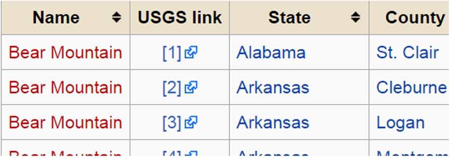
One-sense-per-discourse does not always hold in subject-columns.

The principle of one-sense-per-discourse allows us to treat cells with identical text content as singleton, to build a shared and combined in-table context by including the rows of each cell. As a result, we can create a larger and hence richer feature representation based on the enlarged context. Next, we count the number of features in the feature representation of a cell and use the number as the preference score.

Example 3.

Following Example 2 and assuming that we now need to interpret the non-subject column ‘Director’ (column 3), and the table is complete. By applying the rule of one-sense-per-discourse, we will put the content rows 3, 4 and 7 adjacent to each other, as the target cells (3,3), (4,3) and (7,3) contain identical text ‘Dino Risi’, which we assume to have the same meaning. Then suppose we use the row context of a cell to create a bag-of-words feature representation. The three cells will share the same feature representation, which takes the text content from rows 3, 4 and 7 (excluding the three target cells in question) and applies the bag-of-words transformation. This gives us a bag-of-words representation of 16 features and we use the number 16 as the preference score for the three target cells. We repeat this to other cells in the column, and eventually we re-rank the rows to obtain the table shown in Fig. 6. Another example is shown in Fig. 2 (from data d₂ to d₃).

Fig. 6.

Sample ranking result based on the example table. The three ‘Dino Risi’ cells will have the same feature representation based on the row context highlighted within dashed boxes.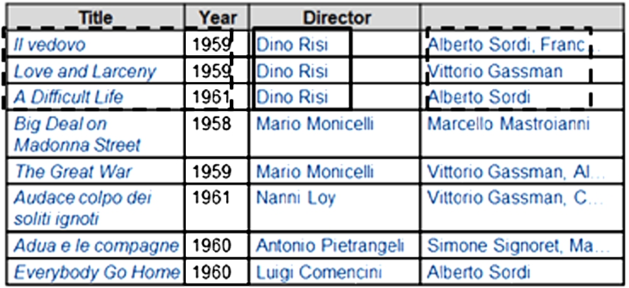

7.2. Preliminary column classification

Next, with the table rows re-arranged by sample ranking, TableMiner⁺ proceeds to classify the column using the I-Inf algorithm. Using Algorithm 1, D contains the ranked list of cells from the column where each element d is an individual cell; for a key-value pair the key (k) is a candidate concept for the column, and the value v is the confidence score. The process operation (line 6) performs cold-start disambiguation of a cell to generate candidate concepts and compute their scores (Section 7.2.1); the update operation (line 7) takes the output of cold-start disambiguation from a cell and updates the set of candidate concepts for the entire column (Section 7.2.2). This repeats until convergence.

7.2.1. Cold-start disambiguation

We first retrieve candidate entities for a cell and then disambiguate the cell based on the similarity between the feature representation of the cell and candidate entities.

Candidate entity generation Given a cell, we search its text content $\mathit{l}\mathrm{(}{\mathit{T}}_{\mathit{i}\mathrm{,}\mathit{j}}\mathrm{)}$ in a knowledge base to retrieve candidate entities ${\mathit{E}}_{\mathit{i}\mathrm{,}\mathit{j}}$ . If a candidate’s name $\mathit{l}\mathrm{(}{\mathit{e}}_{\mathit{i}\mathrm{,}\mathit{j}}\mathrm{)}$ does not have overlap with $\mathit{l}\mathrm{(}{\mathit{T}}_{\mathit{i}\mathrm{,}\mathit{j}}\mathrm{)}$ , the candidate is discarded.

Confidence score of entity Given a candidate entity ${\mathit{e}}_{\mathit{i}\mathrm{,}\mathit{j}}\in {\mathit{E}}_{\mathit{i}\mathrm{,}\mathit{j}}$ , we calculate its confidence score depending on two components: an entity context score ec comparing ${\mathit{e}}_{\mathit{i}\mathrm{,}\mathit{j}}$ and each type of the cell’s context ${\mathit{x}}_{\mathit{i}\mathrm{,}\mathit{j}}\in {\mathit{X}}_{\mathit{i}\mathrm{,}\mathit{j}}$ , and an entity name score en comparing $\mathit{l}\mathrm{(}{\mathit{e}}_{\mathit{i}\mathrm{,}\mathit{j}}\mathrm{)}$ and $\mathit{l}\mathrm{(}{\mathit{T}}_{\mathit{i}\mathrm{,}\mathit{j}}\mathrm{)}$ .

To compare ${\mathit{e}}_{\mathit{i}\mathrm{,}\mathit{j}}$ with the cell’s context ${\mathit{x}}_{\mathit{i}\mathrm{,}\mathit{j}}\in {\mathit{X}}_{\mathit{i}\mathrm{,}\mathit{j}}$ , we compute the overlap between the bag-of-words representation of the candidate entity $\mathit{bow}\mathrm{(}{\mathit{e}}_{\mathit{i}\mathrm{,}\mathit{j}}\mathrm{)}$ and the bag-of-words representation of each context $\mathit{bow}\mathrm{(}{\mathit{x}}_{\mathit{i}\mathrm{,}\mathit{j}}\mathrm{)}$ . To build $\mathit{bow}\mathrm{(}{\mathit{e}}_{\mathit{i}\mathrm{,}\mathit{j}}\mathrm{)}$ , the triples containing ${\mathit{e}}_{\mathit{i}\mathrm{,}\mathit{j}}$ as subject are retrieved from the knowledge base. Then $\mathit{bow}\mathrm{(}{\mathit{e}}_{\mathit{i}\mathrm{,}\mathit{j}}\mathrm{)}$ simply concatenates objects of all triples and transforms them into a bag-of-words.

The context of the cell ${\mathit{X}}_{\mathit{i}\mathrm{,}\mathit{j}}$ contains out-table and in-table context shown in Table 1. Row content concatenates $\mathit{l}\mathrm{(}{\mathit{T}}_{\mathit{i}\mathrm{,}{\mathit{j}}^{\prime }}\mathrm{)}$ where $\mathit{j}\ne {\mathit{j}}^{\prime }$ . These are likely to be attribute data values of entities. Column content concatenates $\mathit{l}\mathrm{(}{\mathit{T}}_{{\mathit{i}}^{\prime }\mathrm{,}\mathit{j}}\mathrm{)}$ where $\mathit{i}\ne {\mathit{i}}^{\prime }$ . These are likely to refer to entities that are semantically similar or related. Column header could contain useful features as entities sometimes use words that indicate its semantic type in its names (e.g., ‘River Sheaf’). Webpage title, table captions/titles and surrounding paragraphs can contain words that are important to entities. Semantic markups may annotate important entities or their attributes on the webpage. They are extracted as RDF triples and the objects of triples that are literals are concatenated.

The overlap between ${\mathit{e}}_{\mathit{i}\mathrm{,}\mathit{j}}$ and any out-table context is computed using a frequency weighted dice function: $$\begin{array}{ll}\hfill \mathit{dice}\mathrm{(}{\mathit{e}}_{\mathit{i}\mathrm{,}\mathit{j}}\mathrm{,}{\mathit{x}}_{\mathit{i}\mathrm{,}\mathit{j}}\mathrm{)}& ={\displaystyle \frac{1}{|\mathit{bow}\mathrm{(}{\mathit{e}}_{\mathit{i}\mathrm{,}\mathit{j}}\mathrm{)}|+|\mathit{bow}\mathrm{(}{\mathit{x}}_{\mathit{i}\mathrm{,}\mathit{j}}\mathrm{)}|}}\\ \hfill & \times [2\times {\displaystyle \sum }_{\mathit{w}\in \mathit{bowset}\mathrm{(}{\mathit{e}}_{\mathit{i}\mathrm{,}\mathit{j}}\mathrm{)}\cap \mathit{bowset}\mathrm{(}{\mathit{x}}_{\mathit{i}\mathrm{,}\mathit{j}}\mathrm{)}}\\ \text{(8)}& \hfill & \times \mathrm{(}\mathit{freq}\mathrm{(}\mathit{w}\mathrm{,}{\mathit{e}}_{\mathit{i}\mathrm{,}\mathit{j}}\mathrm{)}+\mathit{freq}\mathrm{(}\mathit{w}\mathrm{,}{\mathit{x}}_{\mathit{i}\mathrm{,}\mathit{j}}\mathrm{)}\mathrm{)}]\end{array}$$

The overlap between ${\mathit{e}}_{\mathit{i}\mathrm{,}\mathit{j}}$ and any in-table context is measured based on coverage, as intuitively the presence of any in-table features in the bag-of-words representation of a candidate entity is a stronger signal of relevance. $$\begin{array}{ll}\hfill & \mathit{coverage}\mathrm{(}{\mathit{e}}_{\mathit{i}\mathrm{,}\mathit{j}}\mathrm{,}{\mathit{x}}_{\mathit{i}\mathrm{,}\mathit{j}}\mathrm{)}\\ \text{(9)}& \hfill & ={\displaystyle \frac{{\sum }_{\mathit{w}\in \mathit{bowset}\mathrm{(}{\mathit{e}}_{\mathit{i}\mathrm{,}\mathit{j}}\mathrm{)}\cap \mathit{bowset}\mathrm{(}{\mathit{x}}_{\mathit{i}\mathrm{,}\mathit{j}}\mathrm{)}}\mathit{freq}\mathrm{(}\mathit{w}\mathrm{,}{\mathit{x}}_{\mathit{i}\mathrm{,}\mathit{j}}\mathrm{)}}{|\mathit{bow}\mathrm{(}{\mathit{x}}_{\mathit{i}\mathrm{,}\mathit{j}}\mathrm{)}|}}\end{array}$$

Then let $\mathit{overlap}\mathrm{(}{\mathit{e}}_{\mathit{i}\mathrm{,}\mathit{j}}\mathrm{,}{\mathit{x}}_{\mathit{i}\mathrm{,}\mathit{j}}\mathrm{)}$ be the generalized function (either $\mathit{dice}$ or $\mathit{coverage}$ ) that measures overlap between a candidate entity and its source cell’s context ${\mathit{x}}_{\mathit{i}\mathrm{,}\mathit{j}}$ , the entity context score is the weighted sum of the overlap between ${\mathit{e}}_{\mathit{i}\mathrm{,}\mathit{j}}$ and each ${\mathit{x}}_{\mathit{i}\mathrm{,}\mathit{j}}\in {\mathit{X}}_{\mathit{i}\mathrm{,}\mathit{j}}$ : $$\begin{array}{}\text{(10)}& \hfill \mathit{ec}\mathrm{(}{\mathit{e}}_{\mathit{i}\mathrm{,}\mathit{j}}\mathrm{)}={\displaystyle \sum }_{{\mathit{x}}_{\mathit{i}\mathrm{,}\mathit{j}}\in {\mathit{X}}_{\mathit{i}\mathrm{,}\mathit{j}}}\mathit{overlap}\mathrm{(}{\mathit{e}}_{\mathit{i}\mathrm{,}\mathit{j}}\mathrm{,}{\mathit{x}}_{\mathit{i}\mathrm{,}\mathit{j}}\mathrm{)}\times \mathit{wt}\mathrm{(}{\mathit{x}}_{\mathit{i}\mathrm{,}\mathit{j}}\mathrm{)}& \end{array}$$

The entity name score is measured based on the name of ${\mathit{e}}_{\mathit{i}\mathrm{,}\mathit{j}}$ and the text content in ${\mathit{T}}_{\mathit{i}\mathrm{,}\mathit{j}}$ using the standard Dice coefficient as: $$\begin{array}{}\text{(11)}& \mathit{en}\mathrm{(}{\mathit{e}}_{\mathit{i}\mathrm{,}\mathit{j}}\mathrm{)}=\sqrt{{\displaystyle \frac{2\times |\mathit{bowset}\mathrm{(}{\mathit{e}}_{\mathit{i}\mathrm{,}\mathit{j}}\mathrm{)}\cap \mathit{bowset}\mathrm{(}{\mathit{T}}_{\mathit{i}\mathrm{,}\mathit{j}}\mathrm{)}|}{|\mathit{bowset}\mathrm{(}{\mathit{e}}_{\mathit{i}\mathrm{,}\mathit{j}}\mathrm{)}|+|\mathit{bowset}\mathrm{(}{\mathit{T}}_{\mathit{i}\mathrm{,}\mathit{j}}\mathrm{)}|}}}\end{array}$$

Finally, an overall confidence score $\mathit{cf}\mathrm{(}{\mathit{e}}_{\mathit{i}\mathrm{,}\mathit{j}}\mathrm{)}$ is computed using Eq. (12) below. Note that this is different from our previous work [42]. The factor $\sqrt{|\mathit{bow}\mathrm{(}{\mathit{T}}_{\mathit{i}\mathrm{,}\mathit{j}}\mathrm{)}|}$ balances the weight between the candidate entity’s context and name scores by the number of tokens in $\mathit{bow}\mathrm{(}{\mathit{T}}_{\mathit{i}\mathrm{,}\mathit{j}}\mathrm{)}$ . Intuitively, an entity mention that is a long name consisting of multiple tokens (e.g., ‘Harry Potter and the Philosopher’s Stone’) is less likely to be ambiguous than a single-token name (‘Harry’). Therefore the entity name score in the former case should be given higher weight (or conversely, the entity context score is given less weight). When the mention has only a single token, both scores are given the equal weight. $$\begin{array}{}\text{(12)}& \hfill \mathit{cf}\mathrm{(}{\mathit{e}}_{\mathit{i}\mathrm{,}\mathit{j}}\mathrm{)}=\mathit{en}\mathrm{(}{\mathit{e}}_{\mathit{i}\mathrm{,}\mathit{j}}\mathrm{)}+{\displaystyle \frac{\mathit{ec}\mathrm{(}{\mathit{e}}_{\mathit{i}\mathrm{,}\mathit{j}}\mathrm{)}}{\sqrt{|\mathit{bow}\mathrm{(}{\mathit{T}}_{\mathit{i}\mathrm{,}\mathit{j}}\mathrm{)}|}}}& \end{array}$$

Candidate concept generation Then the set of candidate concepts associated with the winning entity are collected and added to the set of candidate concepts for the column ${\mathit{C}}_{\mathit{j}}$ . Mathematically, $$\begin{array}{}\text{(13)}& \hfill {\mathit{C}}_{\mathit{j}}\leftarrow {\displaystyle \bigcup }_{\mathit{i}\in \mathit{I}}\mathit{con}\mathrm{(}{\mathit{e}}_{\mathit{i}\mathrm{,}\mathit{j}}^{+}\mathrm{)}& \end{array}$$ where ${\mathit{e}}_{\mathit{i}\mathrm{,}\mathit{j}}^{+}$ denotes the winning entity for cell ${\mathit{T}}_{\mathit{i}\mathrm{,}\mathit{j}}$ and $\mathit{con}\mathrm{(}{\mathit{e}}_{\mathit{i}\mathrm{,}\mathit{j}}^{+}\mathrm{)}$ returns the set of concepts that the entity belongs to, I is the set of rows to be considered. In case of a sample is used, I includes a subset of rows in the table, otherwise I simply denotes the total number of rows in the table.

Confidence score of concept For each candidate concept, we compute a confidence score based on two components: a concept instance score ce depending on its contributing entities, and a concept context score cc comparing the name of the concept and the context of the header.

The concept instance score of a candidate concept is the sum of the confidence scores of the winning entities on each row where the winning entities elect the candidate concept: $$\begin{array}{}\text{(14)}& \mathit{ce}\mathrm{(}{\mathit{c}}_{\mathit{j}}\mathrm{)}={\displaystyle \frac{{\sum }_{\mathit{i}\in \mathit{I}}\left\{\begin{array}{cc}\mathit{cf}\mathrm{(}{\mathit{e}}_{\mathit{i}\mathrm{,}\mathit{j}}^{+}\mathrm{)}\hfill & \text{if }\mathit{con}\mathrm{(}{\mathit{e}}_{\mathit{i}\mathrm{,}\mathit{j}}^{+}\mathrm{)}\cap \{{\mathit{c}}_{\mathit{j}}\}\ne \varnothing \hfill \\ 0\hfill & \text{else}\hfill \end{array}\right.}{\mathit{I}}}\end{array}$$

Given a candidate concept, if the winning entity on every row $\mathit{i}\in \mathit{I}$ elects the concept, and the confidence score of each of them approaches to 1.0, the concept instance score will approach to the highest of 1.0.

The concept context score is computed in the same principle as entity context score ec using Eq. (10), and the function used to calculate an overlap score between ${\mathit{c}}_{\mathit{j}}$ and each of its context ${\mathit{x}}_{\mathit{j}}\in {\mathit{X}}_{\mathit{j}}$ is the frequency weighted dice function in Eq. (8). This is adapted by replacing ${\mathit{e}}_{\mathit{i}\mathrm{,}\mathit{j}}$ with ${\mathit{c}}_{\mathit{j}}$ and ${\mathit{x}}_{\mathit{i}\mathrm{,}\mathit{j}}$ with ${\mathit{x}}_{\mathit{j}}$ . The out-table context for a column header includes all out-table context shown in Table 1. The in-table context includes all but row content; and column content concatenates all cells ${\mathit{T}}_{\mathit{i}\mathrm{,}\mathit{j}}$ , because entity names can contain indicative words of their semantic types. For $\mathit{bow}\mathrm{(}{\mathit{c}}_{\mathit{j}}\mathrm{)}$ we take the name and URI of the concept and transform them into a bag-of-words.

The final confidence score of a candidate concept $\mathit{cf}\mathrm{(}{\mathit{c}}_{\mathit{j}}\mathrm{)}$ equally combines $\mathit{ce}\mathrm{(}{\mathit{c}}_{\mathit{j}}\mathrm{)}$ and $\mathit{cc}\mathrm{(}{\mathit{c}}_{\mathit{j}}\mathrm{)}$ : $$\begin{array}{}\text{(15)}& \mathit{cf}\mathrm{(}{\mathit{c}}_{\mathit{j}}\mathrm{)}=\mathit{ce}\mathrm{(}{\mathit{c}}_{\mathit{j}}\mathrm{)}+\mathit{cc}\mathrm{(}{\mathit{c}}_{\mathit{j}}\mathrm{)}\end{array}$$

7.2.2. Update candidate concepts for the column

Cold-start disambiguation derives a set of candidate concepts from each cell in a column. If a concept ${\mathit{c}}_{\mathit{j}}$ is new to the column, we create a new key-value pair $⟨{\mathit{c}}_{\mathit{j}}\mathrm{,}\mathit{cf}\mathrm{(}{\mathit{c}}_{\mathit{j}}\mathrm{)}⟩$ and insert it into the set of key-value pairs for the column. If the concept already exists, its concept instance score is re-computed (as it depends on the winning entity from each contributing row) and the overall confidence score is updated accordingly.

7.2.3. Repetition and convergence

The above processes are repeated in the context of I-Inf until convergence is detected by comparing the set of candidate concepts from the current and previous iterations. The end output of this process is ${\mathit{c}}_{\mathit{j}}^{+}$ the winning concept used to annotate the column.

Example 4.

Following Example 3 we continue to classify the ‘Director’ column in the table shown in Fig. 6. Starting from the first cell ‘Dino Risi’, we retrieve candidate entities and compute a confidence score for each. Assuming the winning entity is the Freebase topic ‘fb:/m/0j_nhj’, we then extract its associated concepts and compute confidence score for each concept. Some of the concepts are ‘Film director (fb:/film/director)10 ¹⁰

All examples are superficial and adapted based on real data.

’, ‘Film writer (fb:/film/writer)’, and ‘Award nominee (fb:/award/award_nominee)’. Then as we proceed to the second and third cells, no new concepts are added and the scores of existing concepts are updated. Suppose that the winning entity for the fourth cell is ‘Mario Monicelli (fb:/m/041kw5)’ and the associated concepts are ‘Film writer (fb:/film/writer)’ and ‘TV personality (fb:/tv/tv_personality)’. Here the score of ‘Film writer’ is further updated and ‘TV personality’ is added as candidate concept for the column. Assuming that we reach convergence at this point as the change of scores of candidate concepts compared to the previous iteration is neglectable, and the highest scoring candidate concept is ‘Film writer’. We therefore stop at the fourth cell and annotate the column as ‘Film writer (fb:/film/writer)’.

7.3. Preliminary cell disambiguation

Next, ${\mathit{c}}_{\mathit{j}}^{+}$ is used as constraint to perform preliminary cell disambiguation in the column. The process re-starts from the first cell in the column. For cells that have already passed a cold-start disambiguation process during preliminary column classification, we simply need to re-select the highest scoring candidate entities satisfying the condition: $\mathit{con}\mathrm{(}{\mathit{e}}_{\mathit{i}\mathrm{,}\mathit{j}}\mathrm{)}\cap \{{\mathit{c}}_{\mathit{j}}^{+}\}\ne \varnothing$ . For any new cells, disambiguation follows the same procedure as cold-start disambiguation (Section 7.2.1) with one modification: candidate generation uses ${\mathit{c}}_{\mathit{j}}^{+}$ as a filter to select only entities that are associated with ${\mathit{c}}_{\mathit{j}}^{+}$ as disambiguation candidates. Compared to the exhaustive strategy adopted by state-of-the-art methods, this reduces computation by cutting down the number of candidate entities for consideration.

Disambiguation of each new cell generates a set of concepts, of which some can be new while others may already exists in ${\mathit{C}}_{\mathit{j}}$ . By the end of the process, ${\mathit{C}}_{\mathit{j}}$ is updated by: (1) adding newly derived concepts; (2) for those already exist in ${\mathit{C}}_{\mathit{j}}$ at the beginning, revising their confidence scores. This changes ${\mathit{C}}_{\mathit{j}}$ and in some cases, causes the winning concept for the column to be inconsistent from that at the beginning of the preliminary cell disambiguation stage. This is handled by the UPDATE phase to be discussed in the following section.

Example 5.

Following Example 4, we use ‘Film writer (fb:/film/writer)’ as constraint to disambiguate the cells in the column. For the four cells already processed in Example 4, we simply re-select from their candidate entities the highest scoring one that is also an instance of this concept. To disambiguate the new cell ‘Nanni Loy’, we only consider candidate entities that are instances of the concept for the column:‘Film writer’. Assuming that the winning entity is ‘fb:/m/02qmpfs’. Then its associated concepts ‘Film writer’, ‘Film director (fb:/film/director)’, ‘Film actor (fb:/film/actor)’ are used to further update the candidate concepts on the column. At the end of the process, it is likely that the highest scoring concept for the column has changed to ‘Film director (fb:/film/director)’.

8. NE-column interpretation – The UPDATE phase

Once the LEARNING phase is applied to all NE-columns in the table, the UPDATE phase begins to enforce interdependence between classification and disambiguation within each column as well as across different columns. This is done by an iterative optimization process shown in Algorithm 2. Note that our previous work [42] only captures interdependence between classification and disambiguation within each separate column. Here we improve it by also capturing cross-column interdependence with a notion of ‘domain consensus’.

Algorithm 2

UPDATE

8.1. Domain representation

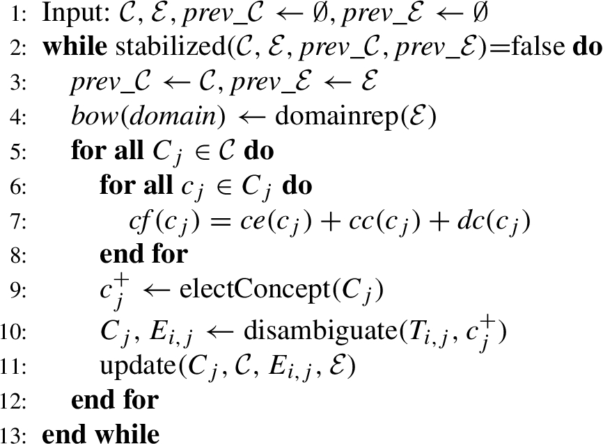
In each iteration, the process starts with creating a bag-of-words representation of the domain using the winning entities from all cells ( $\mathcal{E}$ ) in the table at the current iteration (line 4 in Algorithm 2): $$\begin{array}{}\text{(16)}& \mathit{bow}\mathrm{(}\mathit{domain}\mathrm{)}\leftarrow {\displaystyle \bigcup }_{\mathit{i}\mathrm{,}\mathit{j}}\mathit{defbow}\mathrm{(}{\mathit{e}}_{\mathit{i}\mathrm{,}\mathit{j}}^{+}\mathrm{)}\end{array}$$ where $\mathit{defbow}$ denotes ‘definitional’ bag-of-words, and takes a definitional sentence about an entity and converts it into a bag-of-words representation in the same way as $\mathit{bow}\mathrm{(}·\mathrm{)}$ . A definitional sentence is commonly found in almost any knowledge base. For example, WordNet has a one-sentence definition for every synset; the first sentence in an Wikipedia article usually defines an entity [16]; this also applies to the description of a Freebase topic (e.g., a concept or named entity) or a DBpedia resource. The idea is that the definitional sentence provides a focused description of the entity, likely to contain informative words about the general domain it is related to. In particular, it often contains words forming hypernymy relation with the entity [16,44]. For example, the Freebase definitional sentence about the English city ‘Sheffield’ contains words11

¹¹

http://www.freebase.com/m/0m75g, last retrieved on 13 April 2014.

‘city’, ‘metropolitan’, ‘borough’, ‘Yorkshire’, and ‘England’, which are useful words defining the concept space of the entity.

8.2. Column annotation revision

The bag-of-words representation of the domain is then used to revise the concept annotations on all NE-columns ( $\mathcal{C}$ ). To do so, we compute a domain consensus score dc for each candidate concept from each NE-column, and add this to their overall confidence score (line 7 in Algorithm 2). The domain consensus score is based on the frequency weighted dice overlap between the bag-of-words representations of the concept and the domain. $$\begin{array}{}\text{(17)}& \mathit{dc}\mathrm{(}{\mathit{c}}_{\mathit{j}}\mathrm{)}=\sqrt{\mathit{dice}\mathrm{(}{\mathit{c}}_{\mathit{j}}\mathrm{,}\mathit{domain}\mathrm{)}}\end{array}$$

Since the sizes of $\mathit{bow}\mathrm{(}{\mathit{c}}_{\mathit{j}}\mathrm{)}$ and $\mathit{bow}\mathrm{(}\mathit{domain}\mathrm{)}$ are often different orders of magnitude, square root is used to balance the score. Also domain consensus is computed with respect to entities from all cells from any columns, which serves as a way of ensuring inter-column dependence. After revising the confidence scores of candidate concepts, the winning concepts for each column are re-selected (Line 9).

8.3. Cell annotation revision

For any column, if the new winning concept is different from the that generated in the previous iteration, the disambiguation result on that column is revised (Line 10). This follows the procedure of preliminary cell disambiguation (Section 7.3).

These updating processes are repeated until all annotations are stabilized. Specifically, in each iteration function $\mathit{stabilized}$ checks the winning concepts for all NE-columns and the winning entities for all cells in the previous iteration against those in the current iteration. The UPDATE process is called to be stabilized if no difference is detected.

Note that re-computing disambiguation and classification may require retrieving data of new entity candidates from the knowledge base and subsequently constructing their feature representation for disambiguation due to the possible change of ${\mathit{c}}_{\mathit{j}}^{+}$ at each iteration. However, this design still largely improves the exhaustive strategy because: (1) empirically the UPDATE phase stabilizes fast and in most cases involves merely re-selecting those ‘losing’ candidate entities that were already seen in the LEARNING phase; (2) when new candidates are indeed added it only happens in significantly fewer cells than the entire column that an exhaustive strategy would otherwise have to deal with.

Example 6.

Following Example 5, assuming we have annotated all NE-columns and their cells (also see d₆ in Fig. 2). We begin the UPDATE process by taking the winning entity annotations from columns 1, 3, and 4 in the Table shown in Fig. 6 to create a bag-of-words representation of the domain. Again using the ‘Director’ column, we proceed to compute a domain consensus score for each candidate concept for this column (i.e., ‘Film director’, ‘Film writer’ etc.) and update their confidence scores. The winning concept is re-selected, which we assume is changed to ‘Film director’. This is different from that at the beginning (‘Film writer’). Therefore, we take the new concept and use it to revise cell annotations in the column. We do this for the other two columns and repeat this process until all annotations are no longer changed.

9. Relation enumeration and annotating literal-columns

9.1. Relation enumeration

Relation enumeration firstly begins by interpreting relations between the subject column and any other columns on each row independently. Let ${\mathit{T}}_{\mathit{j}}$ be the subject column in a table and ${\mathit{T}}_{{\mathit{j}}^{\prime }}$ denote any other columns. Given the winning subject entity ${\mathit{e}}_{\mathit{i}\mathrm{,}\mathit{j}}^{+}$ for cell ${\mathit{T}}_{\mathit{i}\mathrm{,}\mathit{j}}$ and ${\mathit{T}}_{\mathit{i}\mathrm{,}{\mathit{j}}^{\prime }}\mathrm{(}\mathit{j}\ne {\mathit{j}}^{\prime }\mathrm{)}$ as another cell on the same row, the candidate set of relations between ${\mathit{T}}_{\mathit{i}\mathrm{,}\mathit{j}}$ and ${\mathit{T}}_{\mathit{i}\mathrm{,}{\mathit{j}}^{\prime }}$ , denoted by ${\mathit{R}}_{\mathit{j}\mathrm{,}{\mathit{j}}^{\prime }}^{\mathit{i}}$ , is derived from the triples containing ${\mathit{e}}_{\mathit{i}\mathrm{,}\mathit{j}}^{+}$ as subject, denoted by ${\mathrm{\Psi }}_{\mathit{i}\mathrm{,}\mathit{j}}=\{⟨{\mathit{e}}_{\mathit{i}\mathrm{,}\mathit{j}}^{+}\mathrm{,}\mathit{predicate}\mathrm{,}\mathit{object}⟩\}$ . Then let ${\mathit{\psi }}_{\mathit{i}\mathrm{,}\mathit{j}}\in {\mathrm{\Psi }}_{\mathit{i}\mathrm{,}\mathit{j}}$ be one of the triples, and functions $\mathit{p}\mathrm{(}{\mathit{\psi }}_{\mathit{i}\mathrm{,}\mathit{j}}\mathrm{)}$ , $\mathit{o}\mathrm{(}{\mathit{\psi }}_{\mathit{i}\mathrm{,}\mathit{j}}\mathrm{)}$ return the predicate and object from the triple respectively, the candidate relations ${\mathit{R}}_{\mathit{j}\mathrm{,}{\mathit{j}}^{\prime }}^{\mathit{i}}$ is the set of unique predicates in ${\mathrm{\Psi }}_{\mathit{i}\mathrm{,}\mathit{j}}$ , i.e., $\{\mathit{p}\mathrm{(}{\mathit{\psi }}_{\mathit{i}\mathrm{,}\mathit{j}}\mathrm{)}|\forall {\mathit{\psi }}_{\mathit{i}\mathrm{,}\mathit{j}}\in {\mathrm{\Psi }}_{\mathit{i}\mathrm{,}\mathit{j}}\}$ .

Then a confidence score is computed for each candidate relation ${\mathit{r}}_{\mathit{j}\mathrm{,}{\mathit{j}}^{\prime }}^{\mathit{i}}\in {\mathit{R}}_{\mathit{j}\mathrm{,}{\mathit{j}}^{\prime }}^{\mathit{i}}$ . To do so, the subset of triples from ${\mathrm{\Psi }}_{\mathit{i}\mathrm{,}\mathit{j}}$ containing ${\mathit{r}}_{\mathit{j}\mathrm{,}{\mathit{j}}^{\prime }}^{\mathit{i}}$ as predicate are selected. Then the object of each triple in this set is matched against the content in ${\mathit{T}}_{\mathit{i}\mathrm{,}{\mathit{j}}^{\prime }}$ using the frequency weighted dice function (Eq. (8)), and the highest score is assigned to be the confidence score for the candidate relation: $$\begin{array}{}\text{(18)}& \hfill \mathit{cf}\mathrm{(}{\mathit{r}}_{\mathit{j}\mathrm{,}{\mathit{j}}^{\prime }}^{\mathit{i}}\mathrm{)}=\underset{{\mathit{\psi }}_{\mathit{i}\mathrm{,}\mathit{j}}\in {\mathrm{\Psi }}_{\mathit{i}\mathrm{,}\mathit{j}}\mathrm{,}\mathit{p}\mathrm{(}{\mathit{\psi }}_{\mathit{i}\mathrm{,}\mathit{j}}\mathrm{)}={\mathit{r}}_{\mathit{j}\mathrm{,}{\mathit{j}}^{\prime }}^{\mathit{i}}}{max}\mathit{dice}\mathrm{(}{\mathit{T}}_{\mathit{i}\mathrm{,}{\mathit{j}}^{\prime }}\mathrm{,}\mathit{o}\mathrm{(}{\mathit{\psi }}_{\mathit{i}\mathrm{,}\mathit{j}}\mathrm{)}\mathrm{)}& \end{array}$$ where function $\mathit{dice}\mathrm{(}{\mathit{T}}_{\mathit{i}\mathrm{,}{\mathit{j}}^{\prime }}\mathrm{,}\mathit{o}\mathrm{(}{\mathit{\psi }}_{\mathit{i}\mathrm{,}\mathit{j}}\mathrm{)}\mathrm{)}$ computes an overlap score between the bag-of-words representations of the cell and the object of a triple that contains ${\mathit{r}}_{\mathit{j}\mathrm{,}{\mathit{j}}^{\prime }}^{\mathit{i}}$ as predicate. The winning relation for the row is denoted by ${\mathit{r}}_{\mathit{j}\mathrm{,}{\mathit{j}}^{\prime }}^{\mathit{i}+}$ .

After the winning relation is computed for each row between ${\mathit{T}}_{\mathit{j}}$ and ${\mathit{T}}_{{\mathit{j}}^{\prime }}$ , the candidate set of relations for the two columns $\mathit{R}\mathrm{(}\mathit{j}\mathrm{,}{\mathit{j}}^{\prime }\mathrm{)}$ is derived by collecting the winning relations on all rows: $$\begin{array}{}\text{(19)}& \mathit{R}\mathrm{(}\mathit{j}\mathrm{,}{\mathit{j}}^{\prime }\mathrm{)}\leftarrow {\displaystyle \bigcup }_{\mathit{i}}{\mathit{r}}_{\mathit{i}\mathrm{,}{\mathit{j}}^{\prime }}^{\mathit{i}+}\end{array}$$

Then a confidence score is computed for each instance ${\mathit{r}}_{\mathit{j}\mathrm{,}{\mathit{j}}^{\prime }}\in \mathit{R}\mathrm{(}\mathit{j}\mathrm{,}{\mathit{j}}^{\prime }\mathrm{)}$ , and it consists of two parts: a relation instance score re and a relation context score. The relation instance score is computed in the same way as concept instance score: $$\begin{array}{}\text{(20)}& \mathit{re}\mathrm{(}{\mathit{r}}_{\mathit{j}\mathrm{,}{\mathit{j}}^{\prime }}\mathrm{)}={\displaystyle \frac{{\sum }_{\mathit{i}}\left\{\begin{array}{cc}\mathit{cf}\mathrm{(}{\mathit{r}}_{\mathit{j}\mathrm{,}{\mathit{j}}^{\prime }}^{\mathit{i}+}\mathrm{)}\hfill & \text{if }{\mathit{r}}_{\mathit{j}\mathrm{,}{\mathit{j}}^{\prime }}^{\mathit{i}+}\equiv {\mathit{r}}_{\mathit{j}\mathrm{,}{\mathit{j}}^{\prime }}\hfill \\ 0\hfill & \text{else}\hfill \end{array}\right.}{|\{{\mathit{T}}_{\mathit{i}}\}|}}\end{array}$$ where i denotes the row index of the table and $|\{{\mathit{T}}_{\mathit{i}}\}|$ returns the number of rows in the table.

The relation context score is computed in the same way as entity context score using Eq. (10), and the function used to calculate an overlap score between ${\mathit{r}}_{\mathit{j}\mathrm{,}{\mathit{j}}^{\prime }}$ and each of its context is the frequency weighted dice function in Eq. (8). This is adapted by replacing ${\mathit{e}}_{\mathit{i}\mathrm{,}\mathit{j}}$ with ${\mathit{r}}_{\mathit{j}\mathrm{,}{\mathit{j}}^{\prime }}$ and ${\mathit{x}}_{\mathit{i}\mathrm{,}\mathit{j}}$ with ${\mathit{x}}_{\mathit{j}\mathrm{,}{\mathit{j}}^{\prime }}$ . The bag-of-words representation $\mathit{bow}\mathrm{(}{\mathit{r}}_{\mathit{j}\mathrm{,}{\mathit{j}}^{\prime }}\mathrm{)}$ is based on $\mathit{l}\mathrm{(}{\mathit{r}}_{\mathit{j}\mathrm{,}{\mathit{j}}^{\prime }}\mathrm{)}$ which returns the name and URI of the relation. The context of a relation includes column header (which sometimes indicates the relation with the subject column), surrounding paragraphs and semantic markups. Other types of context are less likely to contain mentions of relations.

The final confidence score of a candidate relation adds up its instance and context score with equal weights, and the final binary relation that associates subject column ${\mathit{T}}_{\mathit{j}}$ with column ${\mathit{T}}_{\mathit{j}}^{\prime }$ is the candidate with the highest confidence score.

Example 7.

Assuming the entity annotation for cell ${\mathit{T}}_{3\mathrm{,}1}$ in the table of Fig. 6 is ‘A Difficult Life (fb:/m/02qlhz2)’, which has two triples ⟨fb:/m/02qlhz2, fb:/film/film/directed_by, ‘Dino Risi’⟩ and ⟨fb:/m/02qlhz2, fb:/film/film/starring, ‘Dino Sordi’⟩. To predict the relation between columns ${\mathit{T}}_1$ and ${\mathit{T}}_3$ on this row, the object values of the two triples are matched against the text value ‘Dino Risi’ in cell ${\mathit{T}}_{3\mathrm{,}3}$ based on overlap. Then the first triple will receive a score of 1.0 while the second 0.5. Hence the relation between the two columns elected by this row ( ${\mathit{r}}_{1\mathrm{,}3}^{3+}$ ) is the predicate ‘fb:/film/film/directed_by’ and $\mathit{cf}\mathrm{(}{\mathit{r}}_{1\mathrm{,}3}^{3+}\mathrm{)}=1.0$ . Next we repeat this process for the remaining rows to elect a relation for every other row between the two columns, and the set of all these relations become ${\mathit{R}}_{3\mathrm{,}3}$ . Suppose that ${\mathit{r}}_{1\mathrm{,}3}^{4+}$ is also ‘fb:/film/film/directed_by’ and $\mathit{cf}\mathrm{(}{\mathit{r}}_{1\mathrm{,}3}^{4+}\mathrm{)}=0.9$ . Then to compute the overall confidence score of ‘fb:/film/film/directed_by’ across the two columns, the relation instance score adds up the two values and become 1.9. We then calculate the relation context score and add it to the instance score to derive the final score.

9.2. Labeling literal-columns

Literal-columns are expected to contain attribute data of entities in the subject column. They do not denote entities and therefore, cannot be interpreted using the column interpretation method described above. In previous work [7,21,23–25] they are simply ignored. This work also assigns a column annotation that best describes the attribute data in literal-columns.

Given a literal-column ${\mathit{T}}_{\mathit{j}}^{\prime }$ that forms a binary relation ${\mathit{r}}_{\mathit{j}\mathrm{,}{\mathit{j}}^{\prime }}$ with the subject column ${\mathit{T}}_{\mathit{j}}$ , the annotation for this column is simply $\mathit{l}\mathrm{(}{\mathit{r}}_{\mathit{j}\mathrm{,}{\mathit{j}}^{\prime }}\mathrm{)}$ , since ${\mathit{r}}_{\mathit{j}\mathrm{,}{\mathit{j}}^{\prime }}$ typically describes a property of the subject column concept in such cases.

10. Experiment settings

Semantic Table Interpretation can be evaluated by both in-vitro (assessing the annotations directly) and in-vivo (assessing the accuracy of applications built on top of the annotations) experiments. In this work, we use in-vitro experiments because (1) they are the most commonly used evaluation approach and (2) standard datasets are available.

10.1. Knowledge base and datasets

We use Freebase as the knowledge base for Semantic Table Interpretation, as it is currently the largest knowledge base and linked data set in the world. It contains over 3.1 billion facts about over 58 million topics (e.g., entities, concepts), significantly exceeding other popular knowledge bases such as DBpedia and YAGO. Further it has direct mappings to resources from other datasets, making them easier to be used as gold standard. For evaluation, we compiled and annotated four datasets using Freebase: Limaye200, LimayeAll, IMDB and MusicBrainz. To the best of our knowledge, this is the largest dataset for this task and we make them available to encourage comparative studies.12

¹²

Please contact the author on how to obtain, as the dataset is very large. Although Freebase has been closed, this work was however, first submitted in May 2013, at which time the close-down of Freebase was not foreseeable. To enable comparative studies, we also release cached Freebase data for this work. Also the current API on GitHub implements an interface with DBpedia, and a plan is made to migrate relevant software to the Google Knowledge Graph once an appropriate API is available.

10.1.1. LimayeAll and Limaye200

These datasets are the rebuilt versions of the original four datasets used by Limaye et al. [21]. The original datasets consist of over 6,000 tables, 94% collected from Wikipedia and the rest from the general Web. Entities in the tables were annotated with links to Wikipedia articles; columns and binary relations between columns were annotated by concepts and relations in the YAGO knowledge base (2008 version).

These datasets are re-created for a number of reasons. First, Wikipedia has undergone significant changes since the publication of the datasets such that a large proportion of the source webpages – as well as the contained tables – have been changed. Second, we notice that the original ground truth for named entity disambiguation were very sparse and possibly biased. As shown in Appendix C, it is less well-balanced than the re-created dataset and a simple exact name match baseline has achieved significantly higher accuracy than the original reported results in Limaye et al. [21]. Third, this work uses a different knowledge base from YAGO, such that the original ground truth cannot be directly used.

Entity ground truth – LimayeAll We run a process to automatically update the webpages in the original dataset and re-annotate entity cells by mapping the original Wikipedia ground truth to Freebase. Details of this process is described in Appendix B.

Column annotation and relation ground truth – Limaye200 To create the ground truth for evaluating column classification and relation enumeration, a random set of 200 tables are drawn from the LimayeAll dataset. These tables are firstly manually examined to identify subject columns, then annotated following a similar process as Venetis et al. [35]. Specifically, TableMiner⁺ and the baselines (Section 10.3) are run on these tables and the candidate concepts for all table columns and relations between the subject column and other columns in each table are collected and presented to annotators. The annotators mark each label as ‘best’, ‘okay’, or ‘incorrect’. The basic principle is to prefer the most specific concept/relation among all suitable candidates. For example, given a cell ‘Penrith Panthers’, the concept ‘Rugby Club’ is the ‘best’ candidate to label its parent column while ‘Sports Team’ and ‘Organization’ are ‘okay’. The annotators may also insert new labels if none of the candidates are suitable.

10.1.2. IMDB

The IMDB dataset contains over 7,000 tables extracted from a random set of IMDB movie webpages. Each IMDB movie webpage13

¹³

E.g., http://www.imdb.com/title/tt0071562/.

contains a table listing a ‘cast’ column of actors/actresses and a column of corresponding characters played. Cells in the actor/actress column are linked with an IMDB item id, which, when searched in Freebase, returns a unique (if any) mapped Freebase URI. Thus entities in these columns are annotated automatically in such a way. The ‘character’ column is not used since they are not mapped in Freebase. The cast column is also manually labeled with ‘best’ and ‘okay’ concepts in the same way as for Limaye200. No subject column or relations are annotated because only one column is considered in this dataset.

10.1.3. MusicBrainz

The MusicBrainz dataset contains some 1,400 tables extracted from a random set of MusicBrainz record label webpages. Each MusicBrainz record label webpage14

¹⁴

E.g., http://musicbrainz.org/label/9e6b4d7f-4958-4db7-8504-d89e315836af.

contains a table listing the music released by a production company. Each webpage uses pagination to separate very large tables, and only the first page is downloaded. The table typically has 8 columns, of which one lists music release titles (subject column) and one lists music artists. Each release title or artist has a MusicBrainz id, which can be mapped to a Freebase URI in the same way as for the IMDB dataset. Thus entities in these two columns are annotated in such a way. Then the table columns and binary relations between the subject column and others are also annotated manually following the same procedure as for IMDB and Limaye200.

10.1.4. Dataset statistics

Table 3 shows general statistics of the datasets. Figure 7 shows the distribution of rows and columns containing entity annotations in the ground truth, and length of text in cells by number of tokens. Tables in MusicBrainz contain no more than 50 rows because of the pagination on the webpage and only the first page is downloaded. The IMDB entity ground truth has only 1 column in every table; while for MusicBrainz, this is either 1 or 2 columns. Very long cell text is found to be rare in LimayeAll, but slightly more frequent in MusicBrainz due to long names of classic music titles. Cells in IMDB tables are typically person names and usually contains 1 or 2 tokens. Arguably, LimayeAll and Limaye200 are the most diverse datasets, since they cover a significantly larger number of domains and more diverse table structures and schemata, whereas IMDB and MusicBrainz each contains only one table structure and schema.

Table 3

Statistics of the datasets for evaluation. ‘All’ under ‘Labeled columns’ shows the number of both labeled NE- and literal-columns, while ‘NE’ refers to only NE-columns. Likewise ‘All’ under ‘Labeled relations’ shows the number of labeled relations between subject columns and either NE- or literal columns, while ‘NE’ refers to only relations with NE-columns

Dataset	Tables	Subject column	Entities	Labeled columns		Labeled relations
				All	NE	All	NE
Limaye200	200	✓	–	615	415	361	204
LimayeAll	6,310		227,046	–	–	–	–
IMDB	7,416		92,321	7,416	7,416	–	–
MusicBrainz	1,406	✓	93,266	9,842	4,218	7,030	5,624

Fig. 7.

Dataset statistics (min., max. avg. (black diamonds), kth quantile): #r – number of rows; #nec – number of columns containing annotated named entities in ground truth; cl – content cell text length in terms of number of tokens delimited by non-alphanumeric characters.

Table 4 compares against datasets used by other studies. Arguably, TableMiner⁺ is evaluated using the most comprehensive collection of datasets known to date.

Table 4

Comparison against datasets used by state-of-the-art. ‘–’ indicates unknown or not clear

Method	Dataset	Tables	Columns	Entities	Relations
TableMiner+	Limaye200	200	615	–	361
	LimayeAll	6,310	–	227,046	–
	IMDB	7,416	7,416	92,321	–
	MusicBrainz	1,406	9,842	93,266	–
Hignette et al. [14,15]	1 dataset	–	81	–	–
Limaye et al. [21]	4 datasets	6,310	747	142,737	90
Syed et al. [7]	1 dataset	5	21	171	–
Venetis et al. [35]	1 dataset	168	–	–	–
Buche et al. [2]	1 dataset	90	81	–	316
Mulwad et al. [24]	1 dataset	203–490	–	–	–
Zhang [42]	2 datasets	7,446	7,608	94,406	–
Zhang [41]	2 datasets	6,310	615	227,046	–

10.2. Evaluation metrics

Effectiveness – Subject column detection is evaluated by Precision. Then the three annotation tasks of Semantic Table Interpretation are evaluated using the standard Precision, Recall and F1 measures. Since TableMiner⁺ ranks candidates by scores, only the highest ranked prediction by TableMiner⁺ is considered. Each ‘best’ label is awarded a score of 1 while each ‘okay’ label is awarded 0.5. Further, if there are multiple highest-ranked candidates, each candidate considered correct only receives a fraction of its score as $\frac{\mathit{score}}{\mathrm{\#}\mathit{topranked}}$ . For example, if a column containing film titles has two concept candidates with the same highest score: ‘Film’ (best) and ‘Book’ (incorrect), this prediction receives a score of 0.5 instead of 1. This is to penalize the situation where the Semantic Table Interpretation system fails to discriminate false positives from true positives. From a knowledge base population point of view, false positives cause incorrect triples to be populated into knowledge bases and the LOD cloud.

For column classification and relation enumeration, evaluation reports results under both ‘strict’ and ‘tolerant’ mode. To evaluate column classification, the strict mode only considered ‘best’ annotations; while the tolerant mode considers both ‘best’ and ‘okay’ annotations. Evaluating relation enumeration under the strict mode only considers relations between subject column and other columns in a table, and only ‘best’ annotations are included. Under the tolerant mode, in addition to also including ‘okay’ annotations, if TableMiner⁺ predicts correct relations between non-subject columns or the reversed relation between the subject column and other columns, then each prediction is awarded a score of 0.5.

Moreover, since most state-of-the-art methods have focused on only NE-columns, we report results obtained on NE-columns as well as both NE- and literal-columns for column classification and relation enumeration.

The efficiency of TableMiner⁺ is assessed by empirical wall-clock time and savings in terms of candidate entities needed to be considered for disambiguation. As discussed before, retrieving candidate entities and their data, constructing feature space and computing similarities consume the large majority of time. A more reliable way of improving efficiency is thus reducing the size of the candidate space. To reduce network latency we use a caching mechanism in each comparative model and TableMiner⁺ (see Section 10.3). Specifically, when a request to the knowledge base is sent for the first time, we cache the query results locally. Then all subsequent identical requests will only be served by the local cache.

10.3. Comparative models and configurations

TableMiner⁺ is evaluated against four baseline methods and two re-implemented state-of-the-art methods. The implementation of all these methods are released on GitHub.15

¹⁵

https://github.com/ziqizhang/sti.

10.3.1. Baselines

Each baseline starts with the same subject column detection component, but uses different methods for disambiguating entity cells, classifying columns, and annotating relations between subject column and other columns.

Baseline ‘name match’ B _nm firstly disambiguates every cell in an NE-column by retrieving candidate entities from Freebase using the text content in the cell as query, then selecting a single entity: the highest ranked candidate whose name matches exactly the cell text. If no candidates are found to match, the top-ranked candidate is chosen. Freebase adopts a ranking algorithm that reflects both the relevance and popularity of a topic in the knowledge base.

Next, to classify the NE-column with a concept, entities from each cell cast a vote for the concepts they are associated to, and the one receiving the most votes is chosen as the annotation for the column.

Relation enumeration follows a similar procedure. Candidate relations on each row is derived and their scores computed in the same way as TableMiner⁺ (Section 9.1, Eq. (18)). Then each candidate with a score greater than 0 is selected from the row and considered as a candidate relation for the two columns and casts a vote toward the candidate. The best relations for the two columns are those receiving the most votes.

Literal-columns are annotated the same way as TableMiner⁺ (Section 9.2).

Baseline ‘similarity-based’ firstly disambiguates every cell in an NE-column, then derives column annotations based on the winning entity from every cell.

For cell disambiguation, we compute a score for each candidate entity as the sum of a simple context score and the string similarity between the name of the candidate and the cell text. The context score is computed using Eq. (9), where x is the row content only.

For column classification, candidate concepts for an NE-column are firstly gathered based on the winning entities from each cell. The final score of a candidate concept consists of two parts: (1) the number of winning entities associated with the concept normalized by the number of rows in the table, and (2) a string similarity score between the concept’s name and the header text (if exists).

For relation enumeration and the annotation of literal-columns, we use the same procedures from the name match baseline B _nm .

To compute string similarity, we test three metrics and therefore create three similarity baselines: Cosine (B_cos), Dice (B _dice ) coefficient, and Levenshtein (B _lev ).

The key differences between the four baselines and TableMiner⁺ are: (1) TableMiner⁺ uses out-table context while the baselines do not; (2) TableMiner⁺ adopts a bootstrapping, incremental approach with an iterative, recursive optimization process to enforce interdependence between different annotation tasks. The baselines however, use an exhaustive strategy and are based on very simple interdependence (i.e., both relation enumeration and column classification depend on cell disambiguation).

10.3.2. Re-implementation of state-of-the-art

We re-implemented two state-of-the-art methods and adapted them to Freebase as there are no existing software that can be directly used, and also different knowledge bases have been used in the original work. We choose to implement the methods by Limaye et al. [21] and Mulwad et al. [24], as they are able to address all three annotation tasks in Semantic Table Interpretation. Re-implementation of these methods is not a trivial task. First, the use of different knowledge bases implies that certain features used in the original work are unavailable, must be adapted or replaced. Second, each method has used in-house tools for pre-processing or training. Therefore, our re-implementation has focused on the core inference algorithm in the two methods. We advise readers that the re-implementation is not guaranteed to be an identical replication of the original systems. We describe details of re-implementation in Appendix D, and here we summarize key points. Note that both methods can only deal with NE-columns.

Limaye et al. (Limaye2010) model a table as a factor graph and apply joint inference to solve the three annotation tasks simultaneously. A factor encodes the compatibility between a variable (e.g., a cell) and its candidates (e.g., candidate entities), or between variables believed to be interdependent. In the original work, the compatibility is calculated based on a number of features, the weight of which is learned using a supervised model. Our implementation16

¹⁶

We used Mallet GRMM: http://mallet.cs.umass.edu/grmm/.

simply uses equal weights. Further, we discard all relation variables and only build a smaller factor graph of concept and entity variables. This is because empirically, we have noticed that adding relation variables caused drop in the accuracy of column classification (see Appendix D).

Mulwad et al. model a table using a similar factor graph, then apply a light-weight inference algorithm based on semantic message passing. Their method depends on a pre-process that disambiguates entity cells (i.e., the so-called ‘entity ranker’). This process uses a supervised model built on features that are specific to the knowledge bases used in the original work. We create two models each with a different substitute of the ‘entity ranker’. Mulwad2013 uses a simple ranker that linearly combines features equivalent to those used in the original work (but derived from Freebase) to score and rank candidate entities. Mulwad2013 ^tm+ uses TableMiner⁺’s formula of entity confidence score ( $\mathit{cf}\mathrm{(}{\mathit{e}}_{\mathit{i}\mathrm{,}\mathit{j}}\mathrm{)}$ in Section 7.2.1) to score and rank candidate entities.

10.3.3. TableMiner⁺ configuration

The convergence threshold in the I-Inf algorithm is set to 0.0117

¹⁷

This is a rather arbitrary choice that was found to perform reasonably well during development. We did not experiment with different choices extensively.

in both subject column detection and the preliminary column classification phases. The Web search API used for computing the Web search score in subject column detection is the Bing Search API18 ¹⁸

http://datamarket.azure.com/dataset/bing/search.

and default parameters are used. TableMiner⁺ uses various context for Semantic Table Interpretation. The weights of context in different annotation tasks are defined in Table 5.

Table 5

Different context weight used in different components

Component	In-table context			Out-table context
	column header	row content	column content	webpage title	table caption/title	paragraphs	semantic markups
Sub. Col. detection §6.2	–	–	–	1.0	1.0	0.5	–
Entity context score §7.2.1	1.0	1.0	0.5	1.0	1.0	0.5	1.0
Concept context score §7.2.1	1.0	–	1.0	1.0	1.0	1.0	1.0
Relation context score §9.1	1.0	–	–	–	–	1.0	1.0

Context is assigned a weight of 1.0 if it is considered ‘very important’ or 0.5 otherwise (subjectively decided). For example, in subject column detection, if header words are found in the webpage title or table captions, they are stronger indicators (hence ‘very important’) of subject column than if found in paragraphs that are distant from tables. For column classification and relation enumeration, different types of context are equally weighted because the bag-of-words representations for candidate concepts and relations are based on their names – semantically very important features but can be very sparse therefore any matches are considered a strong signal.

In the four datasets, semantic markups are only available in IMDB and MusicBrainz as the Microdata format. Any2319 ¹⁹

https://any23.apache.org/.

is used to extract these annotations as RDF triples and the objects of triples are concatenated to create features. Annotations within the HTML <table> tags are excluded.

10.3.4. Parallelization and hardware

All models except Limaye2010 do not require parallelization as they are reasonably fast. Each model is able to run on a server with 4 GB memory. Limaye2010 requires similarity computation between every pair of candidate entity and concept for each column, the amount of which grows quadratically with respect to the size of a table. Thus the running of Limaye2010 is parallelized on 50 threads, each allocated with 4 GB memory.

11. Results and discussion

11.1. Subject column detection

Table 6 shows the precision of predicting subject columns in the Limaye200 and MusicBrainz datasets. The unsupervised subject column detection method achieves a precision of near 96% and 93% on the Limaye200 and MusicBrainz datasets respectively, compared to the reportedly 94–96% precision by a supervised model in Venetis et al. [35], and therein 83% by a baseline that chooses the leftmost column that does not contain numeric data.

Table 6

Subject column detection results in Precision

Dataset	Tables	Precision
Limaye200	200	95.5
MusicBrainz	1406	92.7

Figure 8 shows the convergence statistics in computing the Web search score (ws) in the I-Inf algorithm. The number of tables in which the ws score is calculated20 ²⁰

In cases that only one NE-column is available in a table, this column is simply selected as the subject column.

is: 145 (73%) in Limaye200, 4,711 (75%) in LimayeAll, and 1,402 (near 100%) in MusicBrainz. Table 7 shows the statistics of the slowest convergence on each dataset.

Fig. 8.

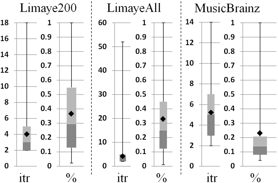
Convergence statistics (max, min, average (black diamond), kth quantiles) for I-Inf in the calculation of the Web search score for subject column detection. itr – number of iterations (rows processed) until convergence; % – fraction of table rows processed.

Table 7

Statistics of the slowest convergence in the calculation of the Web search score for subject column detection

	Limaye200	LimayeAll	MusicBrainz
100% of rows processed in
% of tables	6.9%	5.9%	6.5%
Avg. rows	7.2	6.5	4.6
Rows >20	0	4	0
>50% of rows processed in
% of tables	26.2%	19.8%	12.6%
Avg. rows	6.0	6.0	5.2
Rows >20	0	7	0

Using Limaye200 as an example, Fig. 8 suggests that to compute the ws score, on average, only 4 rows (or less than 35%) are processed, and in 75% of tables no more than 5 rows (or less than 55%) are processed. Table 7 suggests that among all 145 tables that need calculation of ws scores, only 10 tables have all of their rows processed. They have an average of 7.2 rows and none has greater than 20 rows. Then 26.2% of these 145 tables have at least 50% of their rows processed. However, on average they have only 6 rows and none of them have greater than 20 rows. These figures suggest potentially significant improvement in efficiency over an exhaustive approach that computes the ws score using all rows in tables. The figures on the LimayeAll and MusicBrainz datasets suggest even greater savings. Consider that typical Web search APIs are quota-limited and pay-per-use, and it is extremely expensive (if not impossible) to run a local search engine on a reasonable sample of the entire Web. We believe that the I-Inf algorithm delivers substantial benefits in the task of subject column detection.

Manual inspection shows that in most cases the errors fall under several categories. The first is due to duplicate values in subject columns. An extreme example is the disambiguation table discussed before (i.e., ‘List of peaks named Bear Mountain’), in which the subject column contains only a single unique value. The second is caused by long-named entities in subject columns. For example, the subject column in the MusicBrainz tables lists titles of music releases, some of which has a name consisting of more than 10 tokens. This severely penalizes their context match cm and ws scores as it is unlikely to find exact match of their names in table context and search result documents. The third category includes arguable (few) tables that in strict terms, do not necessarily have a subject column. This includes tables listing events, such as lap records of racing car drivers in a particular tournament. In these cases, annotators typically selected the leftmost NE-column.

11.2. Effectiveness

11.2.1. Against baselines

Tables 8, 9 and 10 compare TableMiner⁺ against the four baselines in the cell disambiguation, column classification and relation enumeration tasks respectively. The highest figures are marked in bold. Overall, it is clear that TableMiner⁺ always obtains the best performance in all tasks and on all datasets. It also shows stronger improvement in the classification and relation enumeration tasks.

Table 8

Disambiguation results (F1) on four datasets

	Limaye200	LimayeAll	IMDB	MusicBrainz
${\mathit{B}}_{\mathit{nm}}$	78.3	82.2	92.8	57.0
${\mathit{B}}_{\mathit{lev}}$	78	82.1	93.5	84.83
${\mathit{B}}_{cos}$	79.2	82.7	93.4	84.76
${\mathit{B}}_{\mathit{dice}}$	79.9	82.8	93.5	84.84
TableMiner +	82.3	83.7	97.6	84.87

Table 9

Classification results (F1) on three datasets

			${\mathit{B}}_{\mathit{nm}}$	${\mathit{B}}_{\mathit{lev}}$	${\mathit{B}}_{cos}$	${\mathit{B}}_{\mathit{dice}}$	TableMiner +
Limaye200	NE-columns only	strict	23.9	45.4	43.5	48.9	65.8
		tolerant	48.8	63.8	62.2	66.1	75.0
	All columns	strict	31.4	48.7	46.9	51.3	64.0
		tolerant	51.1	63.3	61.8	65.0	71.5
IMDB	NE-/All columns	strict	22.7	32.3	31.9	32.0	97.0
		tolerant	60.0	64.6	64.4	64.5	97.2
MusicBrainz	NE-columns only	strict	59.1	82.6	83.4	83.9	85.2
		tolerant	61.7	82.6	83.6	83.9	85.9
	All columns	strict	54.6	72.2	72.6	72.9	74.3
		tolerant	55.9	72.2	72.7	72.9	74.7

Table 10

Relation enumeration results (F1) on two datasets

			${\mathit{B}}_{\mathit{nm}}$	${\mathit{B}}_{\mathit{lev}}$	${\mathit{B}}_{cos}$	${\mathit{B}}_{\mathit{dice}}$	TableMiner +
Limaye200	NE-columns only	strict	61.3	61.7	61.8	61.8	72.5
		tolerant	65.8	66.3	66.5	66.4	76.0
	All columns	strict	59.7	61.0	60.6	61.1	66.2
		tolerant	63.0	64.4	64.1	64.4	68.7
MusicBrainz	NE-columns only	strict	63.8	67.2	67.1	67.1	67.9
		tolerant	65.0	68.3	68.2	68.2	69.1
	All columns	strict	78.7	82.0	81.9	81.9	82.6
		tolerant	79.2	82.5	82.4	82.4	83.1

For disambiguation, even the simplistic baseline B _nm obtains surprisingly competitive results on the LimayeAll and IMDB datasets. In fact, on the original datasets by Limaye et al. [21] B _nm obtains a surprisingly high F1 of 92.6, significantly higher than the weighted average21 ²¹

Macro-average over all datasets taking into account the size of each dataset.

of 84.1 based on figures reported in Limaye et al. [21]. As discussed earlier, our analysis – shown in Appendix C – suggests that the original datasets are sparse and less balanced.

Its highly competitive performance on the IMDB dataset could be explained by the domain and the method for ranking search results by Freebase. Movie is a highly popular domain representing a fair large proportion of Freebase. Since Freebase Search API promotes popular topics, when a person name is searched it is more likely to obtain movie-related topics as top results than any other domains. Hence by selecting the top result B _nm is very likely to succeed.

While although music is also a highly popular domain, B _nm could not replicate similar performance. Manual inspection shows that a fair proportion of music titles and artists uses very ambiguous names (e.g., ‘Trouble’, a musical release, ‘Pine’, an artist). In contrast, other baselines perform significantly better by considering row content in tables.

Compared to the baselines, TableMiner⁺ consistently obtains the best performance. On the most diverse dataset LimayeAll, it improves F1 by between 0.9 and 1.5 points. On the MusicBrainz dataset, it makes little difference from B _lev , B_cos, and B _dice . By examining the data it is found that the out-table context on MusicBrainz webpages are very sparse. In most cases, the webpage contains only the table. Microdata annotations are also predominantly found inside table structures, which are not used by TableMiner⁺. On the contrary, the IMDB dataset is completely the opposite: the webpages contain much richer out-table context (including pre-defined Microdata annotations), but little in-table context as the tables have only two columns and neither has column headers. TableMiner⁺ achieves significant improvement (between 3.9 and 4.6) over baselines on IMDB. This strongly suggests that out-table context serves as useful clues for disambiguating entities in table cells, particularly when in-table context is absent. Further, the Microdata-annotations extracted from these webpages could have been a strong contributor considering that the only difference in out-table context used on LimayeAll and IMDB is that the latter also uses them as features.

For classification, TableMiner⁺ in most cases outperforms baselines by a very large margin. Experiments on the most diverse dataset Limaye200 see an improvement of between 16.9 and 41.9 under strict mode and 8.9–26.2 under tolerant mode when only NE-columns are considered. When all columns are included, the figures are 12.7–32.6 strict and 6.5–20.4 tolerant. MusicBrainz sees the smallest improvement of the minimum of 1.3 strict and 2.0 (both v.s. B _dice ) when only NE-columns are considered, or 1.4 strict and 1.8 tolerant when all columns are included. This is due to the same reason behind TableMiner⁺’s moderate performance in the disambiguation task on this dataset: the out-table context is very sparse, thus TableMiner⁺ in most cases only uses in-table context. Again the most significant improvement is obtained on the IMDB dataset. With the lack of in-table context, particularly column headers that are considered a crucial feature in annotating table columns, all baselines perform poorly compared against TableMiner⁺. TableMiner⁺ more than tripled their performance under the strict mode and significantly outperforms under the tolerant mode, achieving near-perfect accuracy in both cases.

Also note that the performance by B _nm is generally inferior on any dataset. This is due to its inability to promote a single top ranked candidate concept in most cases, or in other words, multiple winning candidates are penalized by the scoring method. Other baselines improve this by also considering the string similarity between candidate concept’s label and table column headers.

Table 11

Comparison (F1) against the two re-implemented state-of-the-art (NE-columns only). Note that the re-implementation is not guaranteed to be identical to the original works due to reasons such as the use of specific tools, change of knowledge bases and datasets

			Limaye2010	Mulwad2013	Mulwad2013 tm+	TableMiner +
Disambig.	Limaye200	–	64.3	68.3	80.2	82.3
	LimayeAll	–	66.0	70.1	81.9	83.7
	IMDB	–	80.6	76.0	96.0	97.6
	MusicBrainz	–	66.4	73.4	83.0	84.87
Classification	Limaye200	strict	28.4	30.5	37.4	65.8
		tolerant	51.9	52.3	58.9	75.0
	IMDB	strict	1.7	15.1	59.8	97.0
		tolerant	49.3	55.2	78.2	97.2
	MusicBrainz	strict	72.4	65.6	71.0	85.2
		tolerant	72.4	74.2	79.3	85.9
Relation	Limaye200	strict	–	55.9	55.1	72.5
		tolerant	–	60.5	58.5	76.0
	MusicBrainz	strict	–	60.5	49.5	67.9
		tolerant	–	67.6	62.7	69.1

For relation enumeration, on the multi-domain Limaye200 dataset, an improvement of between 10.7–11.2 strict and 9.5–10.2 tolerant is obtained when only relations between NE-columns are considered. Regardless of column types, the figures are 5.1–6.5 strict and 4.3–5.7 tolerant. Improvement on MusicBrainz is smaller: the minimum of 2.8 strict and 0.8 tolerant with NE-columns only, and the minimum of 0.6 strict and 0.7 tolerant if all columns are included. Again this could be attributed to the lack of out-table context in this dataset.

11.2.2. Against state-of-the-art

Table 11 shows that TableMiner⁺ outperforms the re-implemented state-of-the-art models by a large margin in most cases. Surprisingly, models Limaye2010 and Mulwad2013 have underperformed many baselines in most occasions, particularly in the disambiguation task. This may be attributed to two reasons. First, as discussed before, the original work has used knowledge base specific features that are unavailable in Freebase, or supervised processes to optimize features. This has made the adaptation work difficult and although we have made careful attempt to implement alternatives, we cannot guarantee an identical replication of the original methods. Second, we observe that in the cell disambiguation task, both Limaye2010 and Mulwad2013 have only used features that are based on string similarity metrics. Our similarity baselines (B _lev , B_cos, B _dice ) also use string similarity features but add an important type of feature that proves to be very effective: a context score that compares the bag-of-words representation of candidate entities of a cell against the row context of the cell.

By using the disambiguation component of Table-Miner⁺, Mulwad2013^tm+ made significant improvement over Mulwad2013 on the cell disambiguation and column classification tasks. It also outperforms baselines in several occasions, but still obtained lower accuracy than TableMiner⁺.

The poor performance of all three models on the column classification task under strict mode is mainly due to the fact that the algorithms empirically favored general concepts (‘Person’) over more specific ones (‘Movie Directors’). Again this could be caused by the lack of a clean, strict concept hierarchy that could be more reliable reference of concept specificity than the alternative features we have to use in Freebase. However, concept hierarchies are not necessarily available in all knowledge bases. Nevertheless, TableMiner⁺ is able to predict a single best concept candidate in most cases without such knowledge. Additionally, the extremely poor accuracy on the IMDB dataset under the strict mode is largely because all tables in the dataset share the same schema.

We must re-iterate that despite our best effort, the re-implementation is not identical to the original works due to many reasons stated above. Hence following the practice adopted by Mulwad et al. [24], we also compare against state-of-the-art using reported figures in Table 12. As it is shown, TableMiner⁺ has obtained very competitive results.

Table 12

TableMiner⁺ on Limaye200 (classification and relation enumeration) and LimayeAll (disambiguation) and state-of-the-art reported figures. All results are based on NE-columns only. [24] and [35] report results under tolerant mode only, weighted average are used where necessary

	Disamb.	Class.	Relation
TableMiner strict	83.7	65.8	72.5
TableMiner tolerant		75.0	76.0
Limaye et al. [21]	84.1	44.5	58.3
Mulwad et al. [24]	75.9	54.9	83.5
Venetis et al. [35]	–	68.6	54.8

11.2.3. Remark

Overall, we believe these results are very positive. The rich context model adopted by TableMiner⁺ – especially the usage of out-table context – enables TableMiner⁺ to achieve the best performance in all tasks, and significantly outperform both baseline and state-of-the-art methods that ignore out-table contextual features in most cases. In particular, column classification appears to benefit most, suggesting that out-table context provides very useful clues for annotating table columns. The superior performance observed on the IMDB dataset further confirms this, and also shows that existing semantic markups within webpages can be very useful features in this task. Intuitively, when describing table content we tend to focus on the general information rather than specific data in individual table components, which possibly explains the particular contribution by out-table context to the column classification task. Moreover, results on the IMDB dataset also suggest that TableMiner⁺ can be easily adapted to solve tasks in list structures, which are essentially single column tables without headers.

11.3. Efficiency

Firstly, the efficiency of TableMiner⁺ is compared against the baselines B _lev , B_cos and B _dice that represent the exhaustive strategy. The three baselines are almost identical in terms of efficiency since they only differ in the string similarity metric used. Therefore, only B _lev is compared as an example.

Table 13 compares the wall-clock hours of Table-Miner⁺ against B _lev on the four datasets, and shows the proportion of time spent by TableMiner⁺ on data retrieval – including searching for candidate entities and retrieving their data from Freebase or cache. TableMiner⁺ is shown to be faster than B _lev , despite its complicated feature modeling and algorithmic computation.

Table 13

Wall-clock hours observed for TableMiner⁺ as savings against the baseline ${\mathit{B}}_{\mathit{lev}}$

	Savings (hours)	Savings (% of  ${\mathit{B}}_{\mathit{lev}}$ )	% of time on data retrieval
Limaye200	3.7	21.7%	99%
LimayeAll	45.7	15.2%	97%
IMDB	3.9	4.1%	96%
MusicBrainz	34.3	28.6%	97%

Table 14

Candidate entity reduction in disambiguation operations by TableMiner⁺ compared against exhaustive baseline ${\mathit{B}}_{\mathit{lev}}$ and a would-be exhaustive TableMiner (exh-TableMiner)

	${\mathit{B}}_{\mathit{lev}}$	exh-TableMiner
	Overall	Overall	Constrained Disambiguation phase
Limaye200	48.4%	30.4%	39.2%
LimayeAll	52.2%	32.7%	41.4%
IMDB	10.6%	10.6%	59.4%
MusicBrainz	66.4%	44.3%	50.4%

TableMiner⁺ achieves efficiency improvement by using sample-driven column classification and reducing the number of candidates for cell disambiguation, therefore cutting down both the number of data retrieval and feature construction operations. Specifically, it benefits from two design features. First, the one-sense-per-discourse hypothesis ensures that values repeating on multiple cells in non-NE columns are disambiguated collectively costing only one operation. This avoids both repeated data retrieval and feature construction operations for the same set of entity candidates. Whereas classic methods disambiguate these cells individually, costing extra computation. Second, the bootstrapping approach in TableMiner⁺ reduces the total number of candidate entities by firstly creating preliminary column annotations using a sample instead of the entire column content, then using this outcome to constrain candidate space in entity disambiguation. Table 14 compares the total number of candidate entities processed during disambiguation operations in TableMiner⁺ against (1) the exhaustive baseline B _lev , and (2) a ‘would-be exhaustive TableMiner⁺’ (exh-TableMiner ⁺ ) which exploits one-sense-per-discourse but is forced to disambiguate every unique cell in the column before running column classification (i.e., without using I-Inf to create preliminary column annotations to constrain disambiguation). TableMiner⁺’s improvement is shown as reduction in % against the two reference methods.

Compared against the exhaustive baseline B _lev , TableMiner⁺ reduces the total number of candidate entities to be disambiguated by 10–67%. Note that the smallest improvement on the IMDB dataset is due to (1) the dataset being dominated by very small tables (see Fig. 7 on average less than 15 rows), and as a result, I-Inf in the LEARNING phase does not converge or converges relatively slowly (to be discussed in Appendix E); and (2) one-sense-per-discourse being void since only one column (hence the subject column) is available. Empirically, this translates to the very small improvement in wall-clock time shown in Table 13.

The reduction narrows when compared against exh-TableMiner ⁺ , however it still represents a substantial improvement. If we only consider the new cells to be disambiguated after the preliminary column classification phase, in which case the disambiguation candidate space is constrained by the preliminary column annotations (i.e., ‘constrained disambiguation phase’ in Table 14), TableMiner⁺ improves over exh-TableMiner ⁺ by a significant 39–60%.

Table 15

Number of entity candidates need to be retrieved from Freebase at the UPDATE phase

	Number	‰ of total
Limaye200	177	3.9‰
LimayeAll	7,762	5.1‰
IMDB	418	0.8‰
MusicBrainz	867	1.6‰

Furthermore, as mentioned before, one potential issue that may damage TableMiner⁺’s efficiency is that during the UPDATE phase, new entity candidates can be retrieved and processed, due to the change of winning concepts on a column in each update iteration. In the worst case, the total number of candidates to be retrieved from Freebase equals that in an exhaustive method. However, empirically it is found that this rarely happens. The number of entity candidates to be retrieved from Freebase in the UPDATE phase are shown in Table 15, compared to the total number of new entity candidates retrieved from Freebase by TableMiner⁺ in all phases. Further, Table 16 shows the number of iterations until stabilization is reached in the UPDATE phase. It suggests that the UPDATE phase stabilizes very fast. Compared to the semantic message passing algorithm in Mulwad et al. [24], at high-level, the iterative UPDATE phase is similar to running semantic message passing on a graph containing two types of variable nodes – column headers and content cells – and one type of factor nodes that model compatibility between the variable nodes. This is a much simpler graph than that used by Mulwad et al., which can fail to converge and empirically a threshold must be used to exit the loop.

Table 16

Number of iterations until stabilization at the UPDATE phase. 1 itr – fraction of tables on which the UPDATE phase stabilizes after 1 iteration

	Max.	Avg.	1 itr.
Limaye200	4	1.3	72.8%
LimayeAll	5	1.3	75.8%
IMDB	4	1.2	79.7%
MusicBrainz	4	1.3	73.1%

Secondly, we compare TableMiner⁺ against Limaye2010 and Mulwad2013. To factor out network latency we re-run the three systems using cached Freebase data and compare the wall-clock time. Note that TableMiner⁺ and Mulwad2013 are both run in a single thread while Limaye2010 is run with parallelization using 50 threads. Both Mulwad2013 and Limaye2010 exhaustively process the entire table before running inference algorithms. Table 17 shows that TableMiner⁺ is the most efficient, completing the annotation tasks faster than the other two systems. It is significantly faster than Limaye2010, which spent an enormous amount of time on computing similarity between pairs of entity and concept candidates in each column. The improvement by TableMiner⁺ is rather compelling: had we implemented parallelization for TableMiner⁺, the savings in wall-clock time would be in the orders of magnitude. We believe this is convincing evidence that Semantic Table Interpretation can significantly benefit from efficient algorithms, while parallelization can only be partial solution.

Table 17

Wall-clock hours observed for TableMiner⁺ (1 thread), Mulwad2013 (1 thread), and Limaye2010 (50 threads) when only local cache is used

	Table Miner+	Mulwad 2013	Limaye 2010
LimayeAll	4.6	5.4	76.0
IMDB	2.3	2.5	28.5
MusicBrainz	1.0	1.9	9.0

11.4. The effect of using partial content for interpretation

TableMiner⁺ uses partial content from a table column to perform preliminary column classification, the outcome of which is used to guide preliminary cell disambiguation. The annotations are then revised by the UPDATE process, which allows evidence from the remaining content from the table to feed back into the annotation process. Hence one question that remains to be answered is whether a Semantic Table Interpretation system that is purely based on partial data can be as good as systems that use the entire table content.

To answer this question we carry out additional experiments that are detailed in Appendix E. First, we drop the UPDATE phase from TableMiner⁺ to create a model ${\mathit{TM}}_{\mathit{iinf}}^{\mathit{nu}}$ ( $\mathit{nu}$ means ‘no update’). Effectively, this means that preliminary column classification in ${\mathit{TM}}_{\mathit{iinf}}^{\mathit{nu}}$ will create the final column annotations using a sample from each column, and preliminary cell disambiguation will create the final cell annotations based on the column classification results. Next, we create alternative models by replacing the stopping criteria automatically calculated by I-Inf in ${\mathit{TM}}_{\mathit{iinf}}^{\mathit{nu}}$ with arbitrarily set sample size. For example, we may configure the system to use a maximum of 10 rows from a column in preliminary column classification.

Results have shown that ${\mathit{TM}}_{\mathit{iinf}}^{\mathit{nu}}$ still consistently outperforms the best performing baseline in almost all occasions. Compared against the alternative models using arbitrarily set sample size, it is able to obtain either the best or very close (with a difference of merely 0.1–0.6 point) performance in accuracy. We believe that these further confirm that: (1) Semantic Table Interpretation can benefit from using various in-table and out-table features; (2) it is possible to achieve higher accuracy using only partial data in the task, improving both effectiveness and efficiency; (3) the I-Inf algorithm is very robust as it is able to automatically determine an optimal sample size for column classification.

12. Conclusion

This work introduced TableMiner⁺, a Semantic Table Interpretation method that annotates tabular data for semantic indexing, search and knowledge base population. We have made several contributions to state-of-the-art. First, TableMiner⁺ uses various context both inside and outside tables as features in Semantic Table Interpretation. This is shown to be particularly useful for improving annotation accuracy. Second, TableMiner⁺ is able to make inference based on partial content sampled from a table. This is shown to deliver significant efficiency improvement against state-of-the-art methods that exhaustively process the entire table. Third, TableMiner⁺ offers a comprehensive solution, solving all annotation tasks of Semantic Table Interpretation and deals with both entity and literal columns. And finally, we release the largest collection of datasets as well as the first publicly available software for the task.

Extensive experiments show that TableMiner⁺ outperforms all baselines and re-implemented (near identical) state-of-the-art methods on any datasets under any settings. On the two most diverse datasets covering multiple domains and different table schemata, it significantly improves over all the other models by up to 42 percentage points. Compared against classic, exhaustive baselines, TableMiner⁺ reduces empirical wall-clock time by up to 29% and in the column classification task alone, but uses only 55% of table content (as opposed to 100% by exhaustive methods) to classify columns in the two most diverse datasets. It is also significantly faster than the re-implemented methods even when network latency is eliminated by using a local copy of the knowledge base.

TableMiner⁺ is however, still limited in a number of ways. First, relation enumeration is yet incomplete, as TableMiner⁺ only handles binary relations between the subject column and other columns. Second, several threshold setting (e.g., I-Inf convergence threshold) and weighting in formulas (e.g., subject column score formula) could be improved by using machine learning techniques to learn optimal configurations from data. Third, TableMiner⁺ is evaluated using Freebase, and in the general domain. Plans are made to evaluate it with other knowledge bases such as DBpedia and WikiData, as well as adapting to domain specific contexts. We will explore these directions in the future work.