A hierarchical aggregation framework for efficient multilevel visual exploration and analysis

Abstract

Data exploration and visualization systems are of great importance in the Big Data era, in which the volume and heterogeneity of available information make it difficult for humans to manually explore and analyse data. Most traditional systems operate in an offline way, limited to accessing preprocessed (static) sets of data. They also restrict themselves to dealing with small dataset sizes, which can be easily handled with conventional techniques. However, the Big Data era has realized the availability of a great amount and variety of big datasets that are dynamic in nature; most of them offer API or query endpoints for online access, or the data is received in a stream fashion. Therefore, modern systems must address the challenge of on-the-fly scalable visualizations over large dynamic sets of data, offering efficient exploration techniques, as well as mechanisms for information abstraction and summarization. Further, they must take into account different user-defined exploration scenarios and user preferences. In this work, we present a generic model for personalized multilevel exploration and analysis over large dynamic sets of numeric and temporal data. Our model is built on top of a lightweight tree-based structure which can be efficiently constructed on-the-fly for a given set of data. This tree structure aggregates input objects into a hierarchical multiscale model. We define two versions of this structure, that adopt different data organization approaches, well-suited to exploration and analysis context. In the proposed structure, statistical computations can be efficiently performed on-the-fly. Considering different exploration scenarios over large datasets, the proposed model enables efficient multilevel exploration, offering incremental construction and prefetching via user interaction, and dynamic adaptation of the hierarchies based on user preferences. A thorough theoretical analysis is presented, illustrating the efficiency of the proposed methods. The presented model is realized in a web-based prototype tool, called SynopsViz that offers multilevel visual exploration and analysis over Linked Data datasets. Finally, we provide a performance evaluation and a empirical user study employing real datasets.

1. Introduction

Exploring, visualizing and analysing data is a core task for data scientists and analysts in numerous applications. Data exploration and visualization enable users to identify interesting patterns, infer correlations and causalities, and support sense-making activities over data that are not always possible with traditional data mining techniques [29,54]. This is of great importance in the Big Data era, where the volume and heterogeneity of available information make it difficult for humans to manually explore and analyse large datasets.

One of the major challenges in visual exploration is related to the large size that characterizes many datasets nowadays. Considering the visual information seeking mantra: “overview first, zoom and filter, then details on demand” [94], gaining overview is a crucial task in the visual exploration scenario. However, offering an overview of a large dataset is an extremely challenging task. Information overloading is a common issue in large dataset visualization; a basic requirement for the proposed approaches is to offer mechanisms for information abstraction and summarization.

The above challenges can be overcome by adopting hierarchical aggregation approaches (for simplicity we also refer to them as hierarchical) [36]. Hierarchical approaches allow the visual exploration of very large datasets in a multilevel fashion, offering overview of a dataset, as well as an intuitive and usable way for finding specific parts within a dataset. Particularly, in hierarchical approaches, the user first obtains an overview of the dataset (both structure and a summary of its content) before proceeding to data exploration operations, such as roll-up and drill-down, filtering out a specific part of it and finally retrieving details about the data. Therefore, hierarchical approaches directly support the visual information seeking mantra. Also, hierarchical approaches can effectively address the problem of information overloading as it provides information abstraction and summarization.

A second challenge is related to the availability of API and query endpoints (e.g., SPARQL) for online data access, as well as the cases where that data is received in a stream fashion. The latter pose the challenge of handling large sets of data in a dynamic setting, and as a result, a preprocessing phase, such as traditional indexing, is prevented. In this respect, modern techniques must offer scalability and efficient processing for on-the-fly analysis and visualization of dynamic datasets.

Finally, the requirement for on-the-fly visualization must be coupled with the diversity of preferences and requirements posed by different users and tasks. Therefore, the proposed approaches should provide the user with the ability to customize the exploration experience, allowing users to organize data into different ways according to the type of information or the level of details she wishes to explore.

Considering the general problem of exploring big data [18,43,49,54,80,95], most approaches aim at providing appropriate summaries and abstractions over the enormous number of available data objects. In this respect, a large number of systems adopt approximation techniques (a.k.a. data reduction techniques) in which partial results are computed. Existing approaches are mostly based on: (1) sampling and filtering [2,13,39,55,66,82] and/or (2) aggregation (e.g., binning, clustering) [1,12,36,44,57,58,76,77,89,113]. Similarly, some modern database-oriented systems adopt approximation techniques using query-based approaches (e.g., query translation, query rewriting) [13,57,58,108,114]. Recently, incremental approximation techniques are adopted; in these approaches approximate answers are computed over progressively larger samples of the data [2,39,55]. In a different context, an adaptive indexing approach is used in [118], where the indexes are created incrementally and adaptively throughout exploration. Further, in order to improve performance many systems exploit caching and prefetching techniques [12,25,32,56,60,65,101]. Finally, in other approaches, parallel architectures are adopted [35,55,61,62].

Addressing the aforementioned challenges, in this work, we introduce a generic model that combines personalized multilevel exploration with online analysis of numeric and temporal data. At the core lies a lightweight hierarchical aggregation model, constructed on-the-fly for a given set of data. The proposed model is a tree-based structure that aggregates data objects into multiple levels of hierarchically related groups based on numerical or temporal values of the objects. Our model also enriches groups (i.e., aggregations/summaries) with statistical information regarding their content, offering richer overviews and insights into the detailed data. An additional feature is that it allows users to organize data exploration in different ways, by parameterizing the number of groups, the range and cardinality of their contents, the number of hierarchy levels, and so on. On top of this model, we propose three user exploration scenarios and present two methods for efficient exploration over large datasets: the first one achieves the incremental construction of the model based on user interaction, whereas the second one enables dynamic and efficient adaptation of the model to the user’s preferences. The efficiency of the proposed model is illustrated through a thorough theoretical analysis, as well as an experimental evaluation. Finally, the proposed model is realized in a web-based tool, called SynopsViz that offers a variety of visualization techniques (e.g., charts, timelines) for multilevel visual exploration and analysis over Linked Data (LD) datasets.

Contributions. The main contributions of this work are summarized as follows.

We introduce a generic model for organizing, exploring, and analysing numeric and temporal data in a multilevel fashion.

We implement our model as a lightweight, main memory tree-based structure, which can be efficiently constructed on-the-fly.

We propose two tree structure versions, which adopt different approaches for the data organization.

We describe a simple method to estimate the tree construction parameters, when no user preferences are available.

We define different exploration scenarios assuming various user exploration preferences.

We introduce a method that incrementally constructs and prefetches the hierarchy tree via user interaction.

We propose an efficient method that dynamically adapts an existing hierarchy to a new, considering user’s preferences.

We present a thorough theoretical analysis, illustrating the efficiency of the proposed model.

We develop a prototype system which implements the presented model, offering multilevel visual exploration and analysis over LD.

We conduct a thorough performance evaluation and an empirical user study, using the DBpedia 2014 dataset.

Outline. The remainder of this paper is organized as follows. Section 2 presents the proposed hierarchical model, and Section 3 provides the exploration scenarios and methods for efficient hierarchical exploration. Then, Section 4 presents the SynopsViz tool and demonstrate the basic functionality. The evaluation of our system is presented in Section 5. Section 6 reviews related work, while Section 7 concludes this paper.

2. The HETree model

In this section we present HETree (Hierarchical Exploration Tree), a generic model for organizing, exploring, and analysing numeric and temporal data in a multilevel fashion. Particularly, HETree is defined in the context of multilevel (visual) exploration and analysis. The proposed model hierarchically organize arbitrary numeric and temporal data, without requiring it to be described by an hierarchical scheme. We should note that, our model is not bound to any specific type of visualization; rather it can be adopted by several “flat” visualization techniques (e.g., charts, timeline), offering scalable and multilevel exploration over non-hierarchical data.

In what follows, we present some basic aspects of our working scenario (i.e., visual exploration and analysis scenario) and highlight the main assumptions and requirements employed in the construction of our model. First, the input data in our scenario can be retrieved directly from a database, but also produced dynamically; e.g., from a query or from data filtering (e.g., faceted browsing). Thus, we consider that data visualization is performed online; i.e., we do not assume an offline preprocessing phase in the construction of the visualization model. Second, users can specify different requirements or preferences with respect to the data organization. For example, a user prefers to organize the data as a deep hierarchy for a specific task, while for another task a flat hierarchical organization is more appropriate. Therefore, even if the data is not dynamically produced, the data organization is dynamically adapted to the user preferences. The same also holds for any additional information (e.g., statistical information) that is computed for each group of objects. This information must be recomputed when the groups of objects (i.e., data organization) are modified.

From the above, a basic requirement is that the model must be constructed on-the-fly for any given data and users preferences. Therefore, we implement our model as a lightweight, main memory tree structure, which can be efficiently constructed on-the-fly. We define two versions of this tree structure, following data organization approaches well-suited to visual exploration and analysis context: the first version considers fixed-range groups of data objects, whereas the second considers fixed-size groups. Finally, our structure allows efficient on-the-fly statistical computations, which are extremely valuable for the hierarchical exploration and analysis scenario.

The basic idea of our model is to hierarchically group data objects based on values of one of their properties. Input data objects are stored at the leaves, while internal nodes aggregate their child nodes. The root of the tree represents (i.e., aggregates) the whole dataset. The basic concepts of our model can be considered similar to a simplified version of a static 1D R-Tree [45].

Regarding the visual representation of the model and data exploration, we consider that both data objects sets (leaf nodes contents) and entities representing groups of objects (leaf or internal nodes) are visually represented enabling the user to explore the data in a hierarchical manner. Note that our tree structure organizes data in a hierarchical model, without setting any constraints on the way the user interacts with these hierarchies. As such, it is possible that different strategies can be adopted, regarding the traversal policy, as well as the nodes of the tree that are rendered in each visualization stage.

In the rest of this section, preliminaries are presented in Section 2.1. In Section 2.2, we introduce the proposed tree structure. Sections 2.3 and 2.4 present the two versions of the structure. Finally, Section 2.5 discusses the specification of the parameters required for the tree construction, and Section 2.6 presents how statistics computations can be performed over the tree.

2.1. Preliminaries

In this work we formalize data objects as RDF triples. However, the presented methods are generic and can be applied to any data objects with numeric or temporal attributes. Hence, in the following, the terms triple and (data) object will be used interchangeably.

We consider an RDF dataset R consisting of a set of RDF triples. As input data, we assume a set of RDF triples D, where $\mathit{D}\subseteq \mathit{R}$ and triples in D have as objects either numeric (e.g., integer, decimal) or temporal values (e.g., date, time). Let $\mathit{tr}$ be an RDF triple, $\mathit{tr}.\mathit{s}$ , $\mathit{tr}.\mathit{p}$ and $\mathit{tr}.\mathit{o}$ represent, respectively, the subject, predicate and object of the RDF triple $\mathit{tr}$ .

Given input data D, S is an ordered set of RDF triples, produced from D, where triples are sorted based on objects’ values, in ascending order. Assume that $\mathit{S}[\mathit{i}]$ denotes the i-th triple, with $\mathit{S}[1]$ the first triple. Then, for each $\mathit{i}\mathrm{<}\mathit{j}$ , we have that $\mathit{S}[\mathit{i}].\mathit{o}⩽\mathit{S}[\mathit{j}].\mathit{o}$ . Also, $\mathit{D}=\mathit{S}$ , i.e., for each $\mathit{tr}$ , $\mathit{tr}\in \mathit{D}$ iff $\mathit{tr}\in \mathit{S}$ .

Figure 1 presents a set of 10 RDF triples, representing persons and their ages. In Fig. 1, we assume that the subjects $\mathit{p}0$ – $\mathit{p}9$ are instances of a class Person and the predicate age is a datatype property with integer range.

Fig. 1.

Running example input data (data objects).

Example 1.

In Fig. 1, given the RDF triple $\mathit{tr}=\mathit{p}0\mathit{\text{age }}35$ , we have that $\mathit{tr}.\mathit{s}=\mathit{p}0$ , $\mathit{tr}.\mathit{p}=\mathit{age}$ and $\mathit{tr}.\mathit{o}=35$ . Also, given that all triples comprise the input data D and S is the ordered set of D based on the object values, in ascending order; we have that $\mathit{S}[1]=\mathit{p}8\mathit{age}20$ and $\mathit{S}[10]=\mathit{p}1\mathit{age}100$ .

Assume an interval $\mathit{I}=[\mathit{a}\mathrm{,}\mathit{b}]$ , where $\mathit{a}\mathrm{,}\mathit{b}\in \mathbb{R}$ ; then, $\mathit{I}=\{\mathit{k}\in \mathbb{R}\mid \mathit{a}⩽\mathit{k}⩽\mathit{b}\}$ . Similarly, for $\mathit{I}=[\mathit{a}\mathrm{,}\mathit{b}\mathrm{)}$ , we have that $\mathit{I}=\{\mathit{k}\in \mathbb{R}\mid \mathit{a}⩽\mathit{k}\mathrm{<}\mathit{b}\}$ . Let ${\mathit{I}}^{-}$ and ${\mathit{I}}^{+}$ denote the lower and upper bound of the interval I, respectively. That is, given $\mathit{I}=[\mathit{a}\mathrm{,}\mathit{b}]$ , then ${\mathit{I}}^{-}=\mathit{a}$ and ${\mathit{I}}^{+}=\mathit{b}$ . The length of an interval I is defined as $|{\mathit{I}}^{+}-{\mathit{I}}^{-}|$ .

In this work we assume rooted trees. The number of the children of a node is its degree. Nodes with degree 0 are called leaf nodes. Moreover, any non-leaf node is called internal node. Sibling nodes are the nodes that have the same parent. The level of a node is defined by letting the root node be at level zero. Additionally, the height of a node is the length of the longest path from the node to a leaf. A leaf node has a height of 0.

The height of a tree is the maximum level of any node in the tree. The degree of a tree is the maximum degree of a node in the tree. An ordered tree is a tree where the children of each node are ordered. A tree is called an m-ary tree if every internal node has no more than m children. A full m-ary tree is a tree where every internal node has exactly m children. A perfect m-ary tree is a full m-ary tree in which all leaves are at the same level.

2.2. The HETree structure

In this section, we present in more detail the HETree structure. HETree hierarchically organizes numeric and temporal data into groups; intervals are used to represents these groups.1

¹

Note that our structure handles numeric and temporal data in a similar manner. Also, other types of one-dimensional data may be supported, with the requirement that a total order can be defined over the data.

HETree is defined by the tree degree and the number of leaf nodes.2

²

Note that following a similar approach, the HETree can also be defined by specifying the tree height instead of degree or number of leaves.

Essentially, the number of leaf nodes corresponds to the number of groups where input data objects are organized. The tree degree corresponds to the (maximum) number of groups where a group is split in the lower level.

Given a set of data objects (RDF triples) D, a positive integer ℓ denoting the number of leaf nodes; and a positive integer d denoting the tree degree; an HETree $\mathrm{(}\mathit{D}\mathrm{,}\mathrm{\ell }\mathrm{,}\mathit{d}\mathrm{)}$ is an ordered d-ary tree, with the following basic properties.

• The tree has exactly ℓ number of leaf nodes.

• All leaf nodes appear in the same level.

• Each leaf node contains a set of data objects, sorted in ascending order based on their values. Given a leaf node n, $\mathit{n}.\mathit{data}$ denote the data objects contained in n.

• Each internal node has at most d children nodes. Let n be an internal node, $\mathit{n}.{\mathit{c}}_{\mathit{i}}$ denotes the i-th child for the node n, with $\mathit{n}.{\mathit{c}}_1$ be the leftmost child.

• Each node corresponds to an interval. Given a node n, $\mathit{n}.\mathit{I}$ denotes the interval for the node n.

• At each level, all nodes are sorted based on the lower bounds of their intervals. That is, let n be an internal node, for any $\mathit{i}\mathrm{<}\mathit{j}$ , we have that $\mathit{n}.{\mathit{c}}_{\mathit{i}}.{\mathit{I}}^{-}⩽\mathit{n}.{\mathit{c}}_{\mathit{j}}.{\mathit{I}}^{-}$ .

• For a leaf node, its interval is bounded by the values of the objects included in this leaf node. Let n be the leftmost leaf node; assume that n contains x objects from D. Then, we have that $\mathit{n}.{\mathit{I}}^{-}=\mathit{S}[1].\mathit{o}$ and $\mathit{n}.{\mathit{I}}^{+}=\mathit{S}[\mathit{x}].\mathit{o}$ , where S is the ordered object set resulting from D.

• For an internal node, its interval is bounded by the union of the intervals of its children. That is, let n be an internal node, having k child nodes; then, we have $\mathit{n}.{\mathit{I}}^{-}=\mathit{n}.{\mathit{c}}_1.{\mathit{I}}^{-}$ and $\mathit{n}.{\mathit{I}}^{+}=\mathit{n}.{\mathit{c}}_{\mathit{k}}.{\mathit{I}}^{+}$ .

Furthermore, we present two different approaches for organizing the data in the HETree. Assume the scenario in which a user wishes to (visually) explore and analyse the historic events from DBpedia [8], per decade. In this case, user orders historic events by their date and organizes them into groups of equal ranges (i.e., decade). In a second scenario, assume that a user wishes to analyse in the Eurostat dataset the gross domestic product (GDP) organized into fixed groups of countries. In this case, the user is interested in finding information like: the range and the variance of the GDP values over the top-10 countries with the highest GDP factor. In this scenario, the user orders countries by their GDP and organizes them into groups of equal sizes (i.e., 10 countries per group).

In the first approach, we organize data objects into groups, where the object values of each group covers equal range of values. In the second approach, we organize objects into groups, where each group contains the same number of objects. In the following sections, we present in detail the two approaches for organizing the data in the HETree.

2.3. A content-based HETree (HETree-C)

In this section we introduce a version of the HETree, named HETree-C (Content-based HETree). This HETree version organizes data into equally sized groups. The basic property of the HETree-C is that each leaf node contains approximately the same number of objects and the content (i.e., objects) of a leaf node specifies its interval. For the tree construction, the objects are first assigned to the leaves and then the intervals are defined.

An HETree-C $\mathrm{(}\mathit{D}\mathrm{,}\mathrm{\ell }\mathrm{,}\mathit{d}\mathrm{)}$ is an HETree, with the following extra property. Each leaf node contains λ or $\mathit{\lambda }-1$ objects, where $\mathit{\lambda }=\lceil \frac{|\mathit{D}|}{\mathrm{\ell }}\rceil$ .3

³

We assume that, the number of objects is at least as the number of leaves; i.e., $|\mathit{D}|\ge \mathrm{\ell }$ .

Particularly, the $\mathrm{\ell }-\mathrm{(}\mathit{\lambda }·\mathrm{\ell }-|\mathit{D}|\mathrm{)}$ leftmost leaves contain λ objects, while the rest leaves contain $\mathit{\lambda }-1$ .4

⁴

As an alternative we can construct the HETree-C, so each leaf contains λ objects, except the rightmost leaf which will contain between 1 and λ objects.

We can equivalently define the HETree-C by providing the number of objects per leaf λ, instead of the number of leaves ℓ.

Fig. 2.

A Content-based HETree (HETree-C).

Example 2.

Figure 2 presents an HETree-C constructed by considering the set of objects D from Fig. 1, $\mathrm{\ell }=5$ and $\mathit{d}=3$ . As we can observe, all the leaf nodes contain equal number of objects. Particularly, we have that $\mathit{\lambda }=\lceil \frac{10}{5}\rceil =2$ . Regarding the leftmost interval, we have $\mathit{d}.{\mathit{I}}^{-}=20$ and $\mathit{d}.{\mathit{I}}^{+}=30$ .

2.3.1. The HETree-C construction

We construct the HETree-C in a bottom-up way. Algorithm 1 describes the HETree-C construction. Initially, the algorithm sort the object set D in ascending order, based on objects values (line 1). Then, the algorithm uses two procedures to construct the tree nodes. Finally, the root node of the constructed tree is returned (line 4).

Algorithm 1.

createHETree-C/R (D, ℓ, d)

The constrLeaves-C procedure (Procedure 1) construct ℓ leaf nodes (lines 4–16). For the first k leaves, λ objects are inserted, while for the rest leaves, $\mathit{\lambda }-1$ objects are inserted (lines 6–9). Finally, the set of created leaf nodes is returned (line 17).

Procedure 1.

constrLeaves-C(S, ℓ)

The constrtInterNodes procedure (Procedure 2) builds the internal nodes in a recursive manner. For the nodes H, their parents nodes P are created (lines 4–16); then, the procedure calls itself using as input the parent nodes P (line 21). The recursion terminates when the number of created parent nodes is equal to one (line 17); i.e., the root of the tree is created.

Computational Analysis. The computational cost for the HETree-C construction (Algorithm 1) is the sum of three parts. The first is sorting the input data, which can be done in the worst case in $\mathit{O}\mathrm{(}|\mathit{D}|log|\mathit{D}|\mathrm{)}$ , employing a linearithmic sorting algorithm (e.g., merge-sort). The second part is the constrLeaves-C procedure, which requires $\mathit{O}\mathrm{(}|\mathit{D}|\mathrm{)}$ for scanning all data objects. The third part is the constrtInterNodes procedure, which requires $\mathit{d}·\mathrm{(}\lceil \frac{\mathrm{\ell }}{\mathit{d}}\rceil +\lceil \frac{\mathrm{\ell }}{{\mathit{d}}^2}\rceil +\lceil \frac{\mathrm{\ell }}{{\mathit{d}}^3}\rceil +\cdots +1\mathrm{)}$ , with the sum being the number of internal nodes in the tree. Note that the maximum number of internal nodes in a d-ary tree corresponds to the number of internal nodes in a perfect d-ary tree of the same height. Also, note the number of internal nodes of a perfect d-ary tree of height h is $\frac{{\mathit{d}}^{\mathit{h}}-1}{\mathit{d}-1}$ . In our case, the height of our tree is $\mathit{h}=\lceil {log}_{\mathit{d}}\mathrm{\ell }\rceil$ . Hence, the maximum number of internal nodes is $\frac{{\mathit{d}}^{\lceil {log}_{\mathit{d}}\mathrm{\ell }\rceil }-1}{\mathit{d}-1}⩽\frac{\mathit{d}·\mathrm{\ell }-1}{\mathit{d}-1}$ . Therefore, the constrtInterNodes procedure, in worst case requires $\mathit{O}\mathrm{(}\frac{{\mathit{d}}^2·\mathrm{\ell }-\mathit{d}}{\mathit{d}-1}\mathrm{)}$ . Therefore, the overall computational cost for the HETree-C construction in the worst case is $\mathit{O}\mathrm{(}\mathit{\kappa }log\mathit{\kappa }\mathrm{)}+\mathit{O}\mathrm{(}\mathit{\kappa }\mathrm{)}+\mathit{O}\mathrm{(}\mathit{\kappa }\mathrm{)}=\mathit{O}\mathrm{(}\mathit{\kappa }log\mathit{\kappa }+\mathit{\kappa }+\mathit{\kappa }\mathrm{)}=\mathit{O}\mathrm{(}\mathit{\kappa }log\mathit{\kappa }\mathrm{)}=\mathit{O}\mathrm{(}|\mathit{D}|log|\mathit{D}|\mathrm{)}$ . $\mathit{O}\mathrm{(}|\mathit{D}|log|\mathit{D}|+|\mathit{D}|+\frac{{\mathit{d}}^2·\mathrm{\ell }-\mathit{d}}{\mathit{d}-1}\mathrm{)}=\mathit{O}\mathrm{(}|\mathit{D}|log|\mathit{D}|+\frac{{\mathit{d}}^2·\mathrm{\ell }-\mathit{d}}{\mathit{d}-1}\mathrm{)}$ .5

⁵

In the complexity computations presented through the paper, terms that are dominated by others (i.e., having lower growth rate) are omitted.

Procedure 2.

constrtInterNodes(H, d)

2.4. A range-based HETree (HETree-R)

The second version of the HETree is called HETree-R (Range-based HETree). HETree-R organizes data into equally ranged groups. The basic property of the HETree-R is that each leaf node covers an equal range of values. Therefore, in HETree-R, the data space defined by the objects values is equally divided over the leaves. As opposed to HETree-C, in HETree-R the interval of a leaf specifies its content. Therefore, for the HETree-R construction, the intervals of all leaves are first defined and then objects are inserted.

An HETree-R $\mathrm{(}\mathit{D}\mathrm{,}\mathrm{\ell }\mathrm{,}\mathit{d}\mathrm{)}$ is an HETree, with the following extra property. The interval of each leaf node has the same length; i.e., covers equal range of values. Formally, let S be the sorted RDF set resulting from D, for each leaf node its interval has length ρ, where $\mathit{\rho }=\frac{|\mathit{S}[1].\mathit{o}-\mathit{S}[|\mathit{S}|].\mathit{o}|}{\mathrm{\ell }}$ .6

⁶

We assume here that, there is at least one object in D with different value than the rest objects.

Therefore, for a leaf node n, we have that $|\mathit{n}.{\mathit{I}}^{-}-\mathit{n}.{\mathit{I}}^{+}|=\mathit{\rho }$ . For example, for the leftmost leaf, its interval is $[\mathit{S}[1].\mathit{o}\mathrm{,}\mathit{S}[1].\mathit{o}+\mathit{\rho }\mathrm{)}$ . The HETree-R is equivalently defined by providing the interval length ρ, instead of the number of leaves ℓ.

Example 3.

Figure 3 presents an HETree-R tree constructed by considering the set of objects D (Fig. 1), $\mathrm{\ell }=5$ and $\mathit{d}=3$ . As we can observe from Fig. 3, each leaf node covers equal range of values. Particularly, we have that the interval of each leaf must have length $\mathit{\rho }=\frac{|20-100|}{5}=16$ .

Fig. 3.

A Range-based HETree (HETree-R).

2.4.1. The HETree-R construction

This section studies the construction of the HETree-R structure. The HETree-R is also constructed in a bottom-up fashion.

Similarly with the HETree-C version, Algorithm 1 is used for the HETree-R construction. The only difference is the constrLeaves-R procedure (line 2), which creates the leaf nodes of the HETree-R and is presented in Procedure 3.

The procedure The procedure constructs ℓ leaf nodes (lines 2–9) and assigns same intervals to all of them (lines 4–8), it traverses all objects in S (lines 10–12) and places them to the appropriate leaf node (line 12). Finally, returns the set of created leaves (line 13).

Computational Analysis. The computational cost for the HETree-R construction (Algorithm 1) for sorting the input data (line 1) and creating the internal nodes (line 3) is the same as in the HETree-C case. The constrLeaves-R procedure (line 2) requires $\mathit{O}\mathrm{(}\mathrm{\ell }+|\mathit{D}|\mathrm{)}=\mathit{O}\mathrm{(}|\mathit{D}|\mathrm{)}$ (since $|\mathit{D}|\ge \mathrm{\ell }$ ). Using the computational costs for the first and the third part from Section 2.3.1, we have that in worst case, the overall computational cost for the HETree-R construction is $\mathit{O}\mathrm{(}|\mathit{D}|log|\mathit{D}|+|\mathit{D}|+\frac{{\mathit{d}}^2·\mathrm{\ell }-\mathit{d}}{\mathit{d}-1}\mathrm{)}=\mathit{O}\mathrm{(}|\mathit{D}|log|\mathit{D}|+\frac{{\mathit{d}}^2·\mathrm{\ell }-\mathit{d}}{\mathit{d}-1}\mathrm{)}$ .

Procedure 3.

constrLeaves-R(S, ℓ)

2.5. Estimating the HETree parameters

In our working scenario, the user specifies the parameters required for the HETree construction (e.g., number of leaves ℓ). In this section, we describe our approach for automatically calculating the HETree parameters based on the input data, when no user preferences are provided. Our goal is to derive the parameters by the input data, such that the resulting HETree can address some basic guidelines set by the visualization environment. In what follows, we discuss in detail the proposed approach.

An important parameter in hierarchical visualizations is the minimum and maximum number of objects that can be effectively rendered in the most detailed level.7

⁷

Similar bounds can also be defined for other tree levels.

In our case, the above numbers correspond to the number of objects contained in the leaf nodes. The proper calculation of these numbers is crucial such that the resulting tree avoids overloaded visualizations.

Therefore, in HETree construction, our approach considers the minimum and the maximum number of objects per leaf node, denoted as ${\mathit{\lambda }}_{\mathit{min}}$ and ${\mathit{\lambda }}_{\mathit{max}}$ , respectively. Besides the number of objects rendered in the lowest level, our approach considers perfect m-ary trees, such that a more “uniform” structure (i.e., all the internal nodes have exactly m child nodes) results. The following example illustrates our approach of calculating the HETree parameters.

Example 4.

Assume that based on an adopted visualization technique, the ideal number of data objects to be rendered on a specific screen is between 25 and 50. Hence, we have that ${\mathit{\lambda }}_{\mathit{min}}=25$ and ${\mathit{\lambda }}_{\mathit{max}}=50$ .

Now, let’s assume that we want to visualize the object set ${\mathit{D}}_1$ , using an HETree-C, where $|{\mathit{D}}_1|=500$ . Based on the number of objects and the λ bounds, we can estimate the bounds for the number of leaves. Let ${\mathrm{\ell }}_{\mathit{min}}$ and ${\mathrm{\ell }}_{\mathit{max}}$ denote the lower and the upper bound for the number of leaves. Therefore, we have that $\lceil \frac{|{\mathit{D}}_1|}{{\mathit{\lambda }}_{\mathit{max}}}\rceil ⩽\mathrm{\ell }⩽\lceil \frac{|{\mathit{D}}_1|}{{\mathit{\lambda }}_{\mathit{min}}}\rceil \iff \lceil \frac{500}{50}\rceil ⩽\mathrm{\ell }⩽\lceil \frac{500}{25}\rceil \iff 10⩽\mathrm{\ell }⩽20$ .

Hence, our HETree-C should have between ${\mathrm{\ell }}_{\mathit{min}}=10$ and ${\mathrm{\ell }}_{\mathit{max}}=20$ leaf nodes. Since, we consider perfect m-ary trees, from Table 1 we can identify the tree characteristics that conform to the number of leaves guideline. The candidate setting (i.e., leaf number and degree) is indicated in Table 1, using dark-grey colour. Note that, the settings with $\mathit{d}=2$ are not examined since visualizing two groups of objects in each level is considered a small number under most visualization settings. Hence, in any case we only assume settings with $\mathit{d}⩾3$ and $\mathit{height}⩾2$ . Therefore, an HETree-C with $\mathrm{\ell }=16$ and $\mathit{d}=4$ is a suitable structure for our case.

Now, let’s assume that we want to visualize the object set ${\mathit{D}}_2$ , where $|{\mathit{D}}_2|=1000$ . Following a similar approach, we have that $20⩽\mathrm{\ell }⩽40$ . The candidate settings are indicated in Table 1 using light-grey colour. Hence, we have the following settings that satisfy the considered guideline: S1: $\mathrm{\ell }=27$ , $\mathit{d}=3$ ; S2: $\mathrm{\ell }=25$ , $\mathit{d}=5$ ; and S3: $\mathrm{\ell }=36$ , $\mathit{d}=6$ .

In the case where more than one setting satisfies the considered guideline, we select the preferable one according to following set of rules. From the candidate settings, we prefer the setting which results in the highest tree (1st Criterion).8

⁸

Depending on user preferences and the examined task, the shortest tree may be preferable. For example, starting from the root, the user wishes to access the data objects (i.e., lowest level) by performing the smallest amount of drill-down operations possible.

In case that the highest tree is constructed by more than one settings, we consider the distance c, between ℓ and the centre of ${\mathrm{\ell }}_{\mathit{min}}$ and ${\mathrm{\ell }}_{\mathit{max}}$ (2nd Criterion); i.e., $\mathit{c}=|\mathrm{\ell }-\frac{{\mathrm{\ell }}_{\mathit{min}}+{\mathrm{\ell }}_{\mathit{max}}}{2}|$ . The setting with the lowest c value is selected. Note that, based on the visualization context, different criteria and preferences may be followed.

In our example, from the candidate settings, setting S1 is selected, since it will construct the highest tree (i.e., $\mathit{height}=3$ ). On the other hand, settings S2 and S3 will construct trees with lower heights (i.e., $\mathit{height}=2$ ).

Now, assume a scenario where only S2 and S3 are candidates. In this case, since both settings result to trees with equal heights, the 2nd Criterion is considered. Hence, for the S2 we have ${\mathit{c}}_2=|25-\frac{20+40}{2}|=5$ . Similarly, for the S3 ${\mathit{c}}_3=|36-\frac{20+40}{2}|=6$ . Therefore, between the S2 and S3, the setting S2 is preferable, since ${\mathit{c}}_2\mathrm{<}{\mathit{c}}_3$ .

In case of HETree-R, a similar approach is followed, assuming normal distribution over the values of the objects.

Table 1

Number of leaf nodes for perfect m-ary trees

2.6. Statistics computations over HETree

Data statistics is a crucial aspect in the context of hierarchical visual exploration and analysis. Statistical informations over groups of objects (i.e., aggregations) offer rich insights into the underlying (i.e., aggregated) data. In this way, useful information regarding different set of objects with common characteristics is provided. Additionally, this information may also guide the users through their navigation over the hierarchy.

In this section, we present how statistics computation is performed over the nodes of the HETree. Statistics computations exploit two main aspects of the HETree structure: (1) the internal nodes aggregate their child nodes; and (2) the tree is constructed in bottom-up fashion. Statistics computation is performed during the tree construction; for the leaf nodes, we gather statistics from the objects they contain, whereas for the internal nodes we aggregate the statistics of their children.

For simplicity, here, we assume that each node contains the following extra fields, used for simple statistics computations, although more complex or RDF-related (e.g., most common subject, subject with the minimum value, etc.) statistics can be computed. Assume a node n, as $\mathit{n}.\mathit{N}$ we denote the number of objects covered by n; as $\mathit{n}.\mathit{\mu }$ and $\mathit{n}.{\mathit{\sigma }}^2$ we denote the mean and the variance of the objects’ values covered by n, respectively. Additionally, we assume the minimum and the maximum values, denoted as $\mathit{n}.\mathit{min}$ and $\mathit{n}.\mathit{max}$ , respectively.

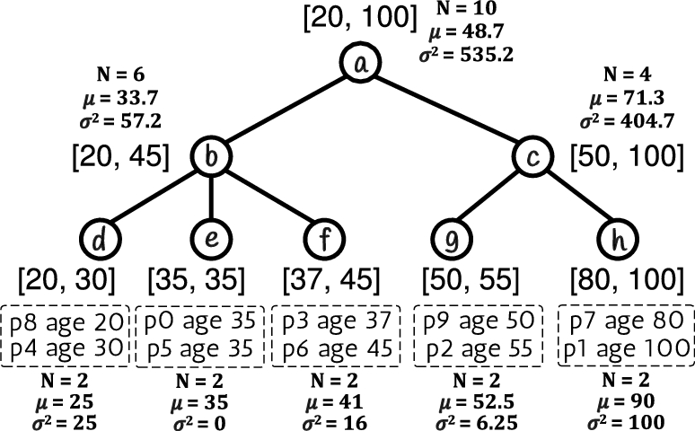
Statistics computations can be easily performed in the construction algorithms (Algorithm 1) without any modifications. The follow example illustrates these computations.

Example 5.

In this example we assume the HETree-C presented in Fig. 2. Figure 4 shows the HETree-C with the computed statistics in each node. When all the leaf nodes have been constructed, the statistics for each leaf is computed. For instance, we can see from Fig. 4, that for the rightmost leaf h we have: $\mathit{h}.\mathit{N}=2$ , $\mathit{h}.\mathit{\mu }=\frac{80+100}{2}=90$ and $\mathit{h}.{\mathit{\sigma }}^2=\frac{1}{2}·\mathrm{(}{\mathrm{(}80-90\mathrm{)}}^2+{\mathrm{(}100-90\mathrm{)}}^2\mathrm{)}=100$ . Also, we have $\mathit{h}.\mathit{min}=80$ and $\mathit{h}.\mathit{max}=100$ . Following the above process, we compute the statistics for all leaf nodes.

Fig. 4.

Statistics computation over HETree.

Then, for each parent node we construct, we compute its statistics using the computed statistics of its child nodes. Considering the c internal node, with the child nodes g and h, we have that $\mathit{c}.\mathit{min}=50$ and $\mathit{c}.\mathit{max}=100$ . Also, we have that $\mathit{c}.\mathit{N}=\mathit{g}.\mathit{N}+\mathit{h}.\mathit{N}=2+2=4$ . Now we will compute the mean value by combining the children mean values: $\mathit{c}.\mathit{\mu }=\frac{\mathit{g}.\mathit{N}·\mathit{g}.\mathit{\mu }+\mathit{h}.\mathit{N}·\mathit{h}.\mathit{\mu }}{\mathit{g}.\mathit{N}+\mathit{h}.\mathit{N}}=\frac{2·52.5+2·90}{2+2}=71.3$ . Similarly, for variance we have $\mathit{c}.{\mathit{\sigma }}^2=\frac{\mathit{g}.\mathit{N}·\mathit{g}.{\mathit{\sigma }}^2+\mathit{h}.\mathit{N}·\mathit{h}.{\mathit{\sigma }}^2+\mathit{g}.\mathit{N}·{\mathrm{(}\mathit{g}.\mathit{\mu }-\mathit{c}.\mathit{\mu }\mathrm{)}}^2+\mathit{h}.\mathit{N}·{\mathrm{(}\mathit{h}.\mathit{\mu }-\mathit{c}.\mathit{\mu }\mathrm{)}}^2}{\mathit{g}.\mathit{N}+\mathit{h}.\mathit{N}}=\frac{2·6.25+2·100+2·{\mathrm{(}52.5-71.3\mathrm{)}}^2+2·{\mathrm{(}90-71.3\mathrm{)}}^2}{2+2}=404.7$ .

The similar approach is also followed for the case of HETree-R.

Computational Analysis. Most of the well known statistics (e.g., mean, variance, skewness, etc.) can be computed linearly w.r.t. the number of elements. Therefore, the computation cost over a set of numeric values S is considered as $\mathit{O}\mathrm{(}|\mathit{S}|\mathrm{)}$ . Assume a leaf node n containing k objects, then the cost for statistics computations for n is $\mathit{O}\mathrm{(}\mathit{k}\mathrm{)}$ . Also, the cost for all leaf nodes is $\mathit{O}\mathrm{(}|\mathit{D}|\mathrm{)}$ . Let an internal node n, then the cost for n is $\mathit{O}\mathrm{(}\mathit{d}\mathrm{)}$ ; since the statistics in n are computed by aggregating the statistics of the d child nodes. Considering that $\frac{\mathit{d}·\mathrm{\ell }-1}{\mathit{d}-1}$ is the maximum number of internal nodes (Section 2.3.1), we have that in the worst case the cost for the internal nodes is $\mathit{O}\mathrm{(}\frac{{\mathit{d}}^2·\mathrm{\ell }-\mathit{d}}{\mathit{d}-1}\mathrm{)}$ . Therefore, the overall cost for statistics computations over an HETree is $\mathit{O}\mathrm{(}|\mathit{D}|+\frac{{\mathit{d}}^2·\mathrm{\ell }-\mathit{d}}{\mathit{d}-1}\mathrm{)}$ .

3. Efficient multilevel exploration

In this section, we exploit the HETree structure in order to efficiently handle different multilevel exploration scenarios. Essentially, we propose two methods for efficient hierarchical exploration over large datasets. The first method incrementally constructs the hierarchy via user interaction; the second one achieves dynamic adaptation of the data organization based on user’s preferences.

3.1. Exploration scenarios

In a typical multilevel exploration scenario, referred here as Basic exploration scenario (BSC), the user explores a dataset in a top-down fashion. The user first obtains an overview of the data through the root level, and then drills down to more fine-grained contents for accessing the actual data objects at the leaves. In BSC, the root of the hierarchy is the starting point of the exploration and, thus, the first element to be presented (i.e., rendered).

The described scenario offers basic exploration capabilities; however it does not assume use cases with user-specified starting points, other than the root, such as starting the exploration from a specific resource, or from a specific range of values.

Consider the following example, in which the user wishes to explore the DBpedia infoboxes dataset to find places with very large population. Initially, she selects the populationTotal property and starts her exploration from the root node, moves down the right part of the tree and ends up at the rightmost leaf that contains the highly populated places. Then, she is interested in viewing the area size (i.e., areaTotal property) for one of the highly populated places and, also, in exploring places with similar area size. Finally, she decides to explore places based on the water area size (i.e., areaWater) they contain. In this case, she prefers to start her exploration by considering places that their water area size is within a given range of values.

In this example, besides BSC one we consider two additional exploration scenarios. In the Resource-based exploration scenario (RES), the user specifies a resource of interest (e.g., an IRI) and a specific property; the exploration starts from the leaf containing the specific resource and proceeds in a bottom-up fashion. Thus, in RES the data objects contained in the same leaf with the resource of interest are presented first. We refer to that leaf as leaf of interest.

The third scenario, named Range-based exploration scenario (RAN) enables the user to start her exploration from an arbitrary point in the hierarchy providing a range of values; the user starts from a set of internal nodes and she can then move up or down the hierarchy. The RAN scenario begins by rendering all sibling nodes that are children of the node covering the specified range of interest; we refer to these nodes as nodes of interest.

Note that, regarding the adopted rendering policy for all scenarios, we only consider nodes belonging to the same level. That is, sibling nodes or data objects contained in the same leaf, are rendered.

Regarding the “navigation-related” operations, the user can move down or up the hierarchy by performing a drill-down or a roll-up operation, respectively. A drill-down operation over a node n enables the user to focus on n and render its child nodes. If n is a leaf node, the set of data objects contained in n are rendered. On the other hand, the user can perform a roll-up operation on a set of sibling nodes S. The parent node of S along with the parent’s sibling nodes are rendered. Finally, the roll-up operation when applied to a set of data objects O will render the leaf node that contains O along its sibling leaves, whereas a drill-down operation is not applied to a data object.

3.2. Incremental HETree construction

In the Web of Data, the dataset might be dynamically retrieved by a remote site (e.g., via a SPARQL endpoint), as a result, in all exploration scenarios, we have assumed that the HETree is constructed on-the-fly at the time the user starts her exploration. In the previous DBpedia example, the user explores three different properties; although only a small part of their hierarchy is accessed, the whole hierarchies are constructed and the statistics of all nodes are computed. Considering the recommended HETree parameters for the employed properties, this scenario requires that 29.5K nodes will be constructed for populationTotal property, 9.8K nodes for the areaTotal and 3.3K nodes for the areaWater, amounting to a total number of 42.6K nodes. However, the construction of the hierarchies for large datasets poses a time overhead (as shown in the experimental section) and, consequently, increased response time in user exploration.

In this section, we introduce ICO (Incremental HETree Construction) method, which incrementally constructs the HETree, based on user interaction. The proposed method goes beyond the incremental tree construction, aiming at further reducing the response time during the exploration process by “pre-constructing” (i.e., prefetching) the parts of the tree that will be visited by the user in her next roll-up or drill-down operation. Hence, a node n is not constructed when the user visits it for the first time; instead, it has been constructed in a previous exploration step, where the user was on a node in which n can be reached by a roll-up or a drill-down operation. This way, our method offers incremental construction of the tree, tailored to each user’s exploration. Finally, we show that, during an exploration scenario, ICO constructs the minimum number of HETree elements.

Fig. 5.

Incremental HETree construction example. Resource-based (RES) exploration scenario; Range-based (RAN) exploration scenario.

Employing ICO method in the DBpedia example, the populationTotal hierarchy will only construct 76 nodes (the root along its child nodes and 9 nodes in each of the lower tree levels) and the areaTotal will construct 3 nodes corresponding to the leaf node containing the requested resource and its siblings. Finally, the areaWater hierarchy initially will contain either 6 or 15 nodes, depending on whether the user’s input range corresponds to a set of sibling leaf nodes, or to a set of sibling internal nodes, respectively.

Example 6.

We demonstrate the functionality of ICO through the following example. Assume the dataset used in our running examples, describing persons and their ages. Figure 5 presents the incremental construction of the HETree presented in Fig. 3 for the RES and RAN exploration scenarios. Blue color is used to indicate the HETree elements that are presented (rendered) to the user, in each exploration stage.

In the RES scenario (upper flow in Fig. 5), the user specifies “http://persons.com/p6” as her resource of interest; all data objects contained in the same leaf (i.e., e) with the resource of interest are initially presented to the user. The ICO initially constructs the leaf e, along with its siblings, i.e., leaves d and f. These leaves correspond to the nodes that the user can reach in a next (roll-up) step. Next, the user rolls up and the leaves d, e and f are presented to her. At the same time, parent node b and its sibling c are constructed. Note that all elements which are accessible to the user by moving either down (i.e., d, e, f data objects), or up (i.e., b, c nodes) are already constructed. Finally, when the user rolls up b and c nodes are rendered and parent node a, along with the children of c, i.e., g and h, are constructed.

In the RAN scenario (lower flow in Fig. 5), the user specifies $[30\mathrm{,}50]$ as her range of interest. The nodes covering this range (i.e., d, e) are initially presented along with their sibling f. Also, ICO constructs the parent node b and its sibling c because they are accessible by one exploration step. Then, the user performs a roll-up and ICO constructs the a, g, h nodes (as described in the RES scenario above).

In the beginning of each exploration scenario, ICO constructs a set of initial nodes, which are the nodes initially presented, as well as the nodes potentially reached by the user’s first operation (i.e., required HETree elements). The required HETree elements of an exploration step are nodes that can be reached by the user by performing one exploration operation. Hence, in the RES scenario, the initial nodes are the leaf of interest and its sibling leaves. In the RAN, the initial nodes are the nodes of interest, their children, and their parent node along with its siblings. Finally, in the BSC scenario the initial nodes are the root node and its children.

In what follows we describe the construction rules adopted by ICO through the user exploration process. These rules provide the correspondences between the types of elements presented in each exploration step and the elements that ICO constructs. Note that these rules are applied after the construction of the initial nodes, in all three exploration scenarios. The correctness of these rules is verified later in Proposition 1.

Rule 1.

If a set of internal sibling nodes C is presented, ICO constructs: (i) the parent node of C along with the parent’s siblings, and (ii) the children of each node in C.

Rule 2.

If a set of leaf sibling nodes L is presented, ICO does not construct anything (the required nodes have been previously constructed).

Rule 3.

If a set of data objects O is presented, ICO does not construct anything (the required nodes have been previously constructed).

The following proposition shows that, in all case, the required HETree elements have been constructed earlier by ICO.9

⁹

Proofs are included in Appendix A.

Proposition 1.

In any exploration scenario, the HETree elements a user can reach by performing one operation (i.e., required elements), have been previously constructed by ICO.

Also, the following theorem shows that over any exploration scenario ICO constructs only the required HETree elements.

Theorem 1.

ICO constructs the minimum number of HETree elements in any exploration scenario.

3.2.1. ICO algorithm

In this section, we present the incremental HETree construction algorithm. Note that, here we include the pseudocode only for the HETree-R version, since the only difference with the HETree-C version is in the way that the nodes’ intervals are computed and that the dataset is initially sorted. In the analysis of the algorithms, both versions are studied.

Here, we assume that each node n contains the following extra fields. Let a node n, $\mathit{n}.\mathit{p}$ denotes the parent node of n, and $\mathit{n}.\mathit{h}$ denotes the height of n in the hierarchy. Additionally, given a dataset D, $\mathit{D}.\mathit{minv}$ and $\mathit{D}.\mathit{maxv}$ denote the minimum and the maximum value for all objects in D, respectively. The user preferences regarding the exploration’s starting point are represented as an interval U. In the RES scenario, given that the value of the explored property for the resource of interest is o, we have ${\mathit{U}}^{-}={\mathit{U}}^{+}=\mathit{o}$ . In the RAN scenario, given that the range of interest is R, we have that ${\mathit{U}}^{-}=max\mathrm{(}\mathit{D}.\mathit{minv}\mathrm{,}{\mathit{R}}^{-}\mathrm{)}$ and ${\mathit{U}}^{+}=min\mathrm{(}\mathit{D}.\mathit{maxv}\mathrm{,}{\mathit{R}}^{+}\mathrm{)}$ . In the BSC scenario, the user does not provide any preferences regarding the starting point, so we have ${\mathit{U}}^{-}=\mathit{D}.\mathit{minv}$ and ${\mathit{U}}^{+}=\mathit{D}.\mathit{maxv}$ . Finally, according to the definition of HETree, a node n encloses a data object (i.e., triple) $\mathit{tr}$ if $\mathit{n}.{\mathit{I}}^{-}⩾\mathit{tr}.\mathit{o}$ and $\mathit{n}.{\mathit{I}}^{+}⩽\mathit{tr}.\mathit{o}$ .

The algorithm ICO-R (Algorithm 2) implements the incremental method for HETree-R. The algorithm uses two procedures to construct all required nodes (available in Appendix B). The first procedure constrRollUp-R (Procedure 4) constructs the nodes which can be reached by a roll-up operation, whereas constrDrillDown-R (Procedure 5) constructs the nodes which can be reached by a drill-down operation. Additionally, the aforementioned procedures exploit two secondary procedures (Appendix B): computeSiblingInterv-R (Procedure 6) and constrSiblingNodes-R (Procedure 7), which are used for nodes’ intervals computations and nodes construction.

Algorithm 2.

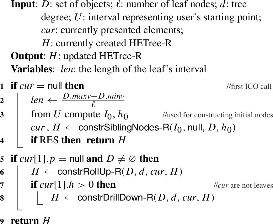
ICO-R(D, ℓ, d, U, $\mathit{cur}$ , H)

The ICO-R algorithm is invoked at the beginning of the exploration scenario, in order to construct the initial nodes, as well as every time the user performs an operation. The algorithm takes as input the dataset D, the tree parameters d and ℓ, the starting point U, the currently presented (i.e., rendered) elements $\mathit{cur}$ , and the constructed HETree H. ICO-R begins with the currently presented elements $\mathit{cur}$ equal to $\mathit{null}$ (lines 1–5). Based on the starting point U, the algorithm computes the interval ${\mathit{I}}_0$ corresponding to the sibling nodes that are first presented to the user, as well as its hierarchy height ${\mathit{h}}_0$ (line 3). For sake of simplicity, the details for computing ${\mathit{I}}_0$ and ${\mathit{h}}_0$ are omitted. For example, the interval I for the leaf that contains the resource of interest with object value o, is computed as ${\mathit{I}}^{-}=\mathit{D}.\mathit{minv}+\mathit{len}·\lfloor \frac{\mathit{o}-\mathit{D}.\mathit{minv}}{\mathit{len}}\rfloor$ and ${\mathit{I}}^{+}=min\mathrm{(}\mathit{D}.\mathit{maxv}\mathrm{,}{\mathit{I}}^{-}+\mathit{len}\mathrm{)}$ . Following a similar approach, we can easily compute ${\mathit{I}}_0$ and ${\mathit{h}}_0$ .

Based on ${\mathit{I}}_0$ , the algorithm constructs the sibling nodes that are first presented to the user (line 4). Then, the algorithm constructs the rest initial nodes (lines 6–9). In the RES case, as ${\mathit{I}}_0$ we consider the interval that includes the leaf that contains the resource of interest along with its sibling leaves. Hence, all the initial nodes are constructed in line 4 and the algorithm terminates (line 5) until the next user’s operation.

After the first call, in each ICO execution, the algorithm initially checks if the parent node of the currently presented elements is already constructed, or if all the nodes that enclose data objects10

¹⁰

Note that in the HETree-R version, we may have nodes that do not enclose any data objects.

have been constructed (line 6). Then, procedure constrRollUp-R (line 7) is used to construct the $\mathit{cur}$ parent node, as well as the parent’s siblings. In the case that $\mathit{cur}$ are not leaf nodes or data objects (line 8), procedure constrDrillDown-R (line 9) is used to construct all $\mathit{cur}$ children. Finally, the algorithm returns the updated HETree (line 10).

3.2.2. Computational analysis

Here we analyse the incremental construction for both HETree versions.

Number of Constructed Nodes. Regarding the number of initial nodes constructed in each scenario: in RES scenario, at most d leaf nodes are constructed; in RAN scenario, at most $2\mathit{d}+{\mathit{d}}^2$ nodes are constructed; finally in BSC scenario, $\mathit{d}+1$ are constructed.

Regarding the maximum number of nodes constructed in each operation in RES and RAN scenarios: (1) A roll-up operation constructs at most $\mathit{d}+\mathit{d}·\mathrm{(}\mathit{d}-1\mathrm{)}={\mathit{d}}^2$ nodes. The d nodes are constructed in constrRollUp, whereas the $\mathit{d}·\mathrm{(}\mathit{d}-1\mathrm{)}$ in constrDrillDown. (2) A drill-down operation constructs at most ${\mathit{d}}^2$ nodes in constrDrillDown. As for the BSC scenario: (1) A roll-up operation does not construct any nodes. (2) A drill-down operation constructs at most ${\mathit{d}}^2$ nodes in constrDrillDown.

Discussion. The worst case for the computational cost is higher in HETree-R than in HETree-C, for all exploration scenarios. Particularly, in HETree-R worst case, ICO must build leaves that contain the whole dataset and the computational cost is $\mathit{O}\mathrm{(}|\mathit{D}|log|\mathit{D}|\mathrm{)}$ for all scenarios. In HETree-C, for the RES and RAN scenarios, the cost is $\mathit{O}\mathrm{(}{\mathit{d}}^2+\frac{\mathit{d}-1}{\mathit{d}}|\mathit{D}|\mathrm{)}$ , and for the BSC scenario the cost is $\mathit{O}\mathrm{(}{\mathit{d}}^2+|\mathit{D}|\mathrm{)}$ . A detailed computational analysis for both HETree-R and HETree-C is included in Appendix C.

Table 2

Summary of Adaptive HETree Construction^⋆

3.3. Adaptive HETree construction

In a (visual) exploration scenario, users wish to modify the organization of the data by providing user-specific preferences for the whole hierarchy or part of it. The user can select a specific subtree and alter the number of groups presented in each level (i.e., the tree degree) or the size of the groups (i.e., number of leaves). In this case, a new tree (or a part of it) pertaining to the new parameters provided by the user should be constructed on-the-fly.

For example, consider the HETree-C of Fig. 6 representing ages of persons.11

¹¹

For simplicity, Fig. 6 presents only the values of the objects.

A user may navigate to node b, where she prefers to increase the number of groups presented in each level. Thus, she modifies the degree of b from 2 to 4 and the subtree is adapted to the new parameter as depicted on the bottom tree of Fig. 6. On the other hand, the user prefers exploring the right subtree (starting from node c) with less details. She chooses to increase the size of the groups by reducing (from 4 to 2) the number of leaves for the subtree of c. In both cases, constructing the subtree from scratch based on the user-provided parameters and recomputing statistics entails a significant time overhead, especially, when user preferences are applied to a large part of or the whole hierarchy.

Fig. 6.

Adaptive HETree example.

In this section, we introduce ADA (Adaptive HETree Construction) method, which dynamically adapts an existing HETree to a new, considering a set of user-defined parameters. Instead of both constructing the tree and computing the nodes’ statistics from scratch, our method reconstructs the new part(s) of the hierarchy by exploiting the existing elements (i.e., nodes, statistics) of the tree. In this way, ADA achieves to reduce the overall construction cost and enables the on-the-fly reorganization of the visualized data. In the example of Fig. 6, the new subtree of b can be derived from the old one, just by removing the internal nodes d and e, while the new subtree of c results from merging leaves together and aggregating their statistics.

Let $\mathcal{T}\mathrm{(}\mathit{D}\mathrm{,}\mathrm{\ell }\mathrm{,}\mathit{d}\mathrm{)}$ denote the existing HETree and ${\mathcal{T}}^{\prime }\mathrm{(}\mathit{D}\mathrm{,}{\mathrm{\ell }}^{\prime }\mathrm{,}{\mathit{d}}^{\prime }\mathrm{)}$ is the new HETree corresponding to the new user preferences for the tree degree ${\mathit{d}}^{\prime }$ and the number of leaves ${\mathrm{\ell }}^{\prime }$ . Note that $\mathcal{T}$ could also denote a subtree of an existing HETree (in the scenario where the user modifies only a part of it). In this case, the user indicates the reconstruction root of $\mathcal{T}$ .

Then, ADA identifies the following elements of $\mathcal{T}$ : (1) The elements of $\mathcal{T}$ that also exist in ${\mathcal{T}}^{\prime }$ . For example, consider the following two cases: the leaf nodes of ${\mathcal{T}}^{\prime }$ are internal nodes of $\mathcal{T}$ in level x; the statistics of ${\mathcal{T}}^{\prime }$ nodes in level x are equal to the statistics of $\mathcal{T}$ nodes in level y. (2) The elements of $\mathcal{T}$ that can be reused (as “building blocks”) for constructing elements in ${\mathcal{T}}^{\prime }$ . For example, consider the following two cases: each leaf node of ${\mathcal{T}}^{\prime }$ is constructed by merging x leaf nodes of $\mathcal{T}$ ; the statistics for the node n of ${\mathcal{T}}^{\prime }$ can be computed by aggregating the statistics from the nodes q and w of $\mathcal{T}$ .

Consequently, we consider that an element (i.e., node or node’s statistics) in ${\mathcal{T}}^{\prime }$ can be: (1) constructed/computed from scratch,12

¹²

Note that it is possible for a from scratch constructed node in ${\mathcal{T}}^{\prime }$ to aggregate statistics from nodes in $\mathcal{T}$ .

(2) reused as is from $\mathcal{T}$ or (3) derived by aggregating elements from  $\mathcal{T}$ .

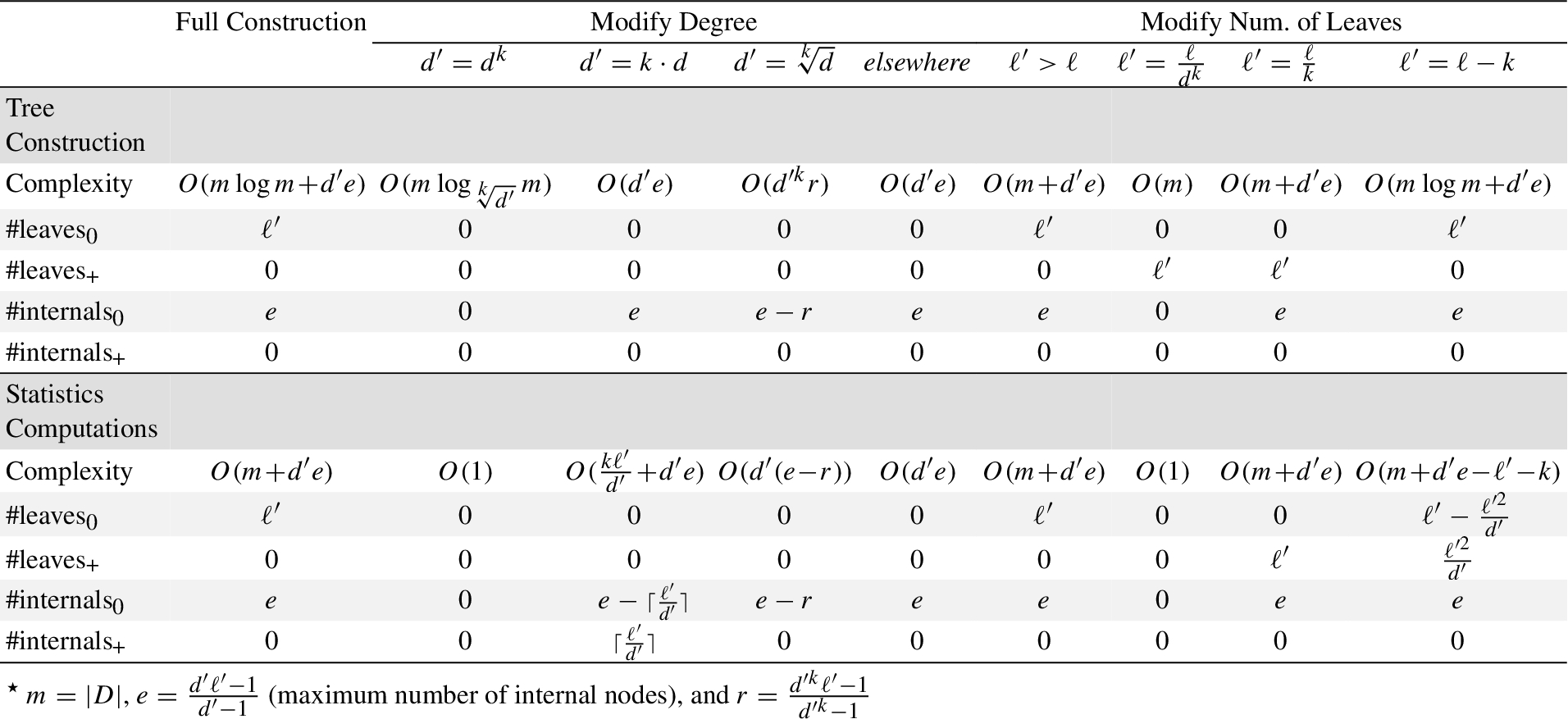
Table 2 summarizes the ADA reconstruction process. Particularly, the table includes: (1) the computational complexity for constructing ${\mathcal{T}}^{\prime }$ , denoted as Complexity; (2) the number of leaves and internal nodes of ${\mathcal{T}}^{\prime }$ constructed from scratch, denoted as $\mathrm{\#}{\mathit{leaves}}_0$ and $\mathrm{\#}{\mathit{internals}}_0$ , respectively; and (3) the number of leaves and internal nodes of ${\mathcal{T}}^{\prime }$ derived from nodes of $\mathcal{T}$ , denoted as $\mathrm{\#}{\mathit{leaves}}_{+}$ and $\mathrm{\#}{\mathit{internals}}_{+}$ , respectively. The lower part of the table presents the results for the computation of node statistics in ${\mathcal{T}}^{\prime }$ . Finally, the second table column, denoted as Full Construction, presents the results of constructing ${\mathcal{T}}^{\prime }$ from scratch.

The following example demonstrates the ADA results, considering a DBpedia exploration scenario.

Example 7.

The user explores the populationTotal property of the DBpedia dataset. The default system organization for this property is a hierarchy with degree 3. The user modifies the tree parameters in order to fit better visualization results as following. First, she decides to render more groups in each hierarchy level and increases the degree from 3 to 9 (1st Modification). Then, she observes that the results overflow the visualization area and that a smaller degree fits better; thus she re-adjusts the tree degree to a value of 6 (2nd Modification). Finally, she navigates through the data values and decides to increase the groups’ size by a factor of three (i.e., dividing by three the number of leaves) (3rd Modification). Again, she corrects her decision and readjusts the final group size to twice the default size (4th Modification).

Table 3 summarizes the number of nodes, constructed by a Full Construction and ADA in each modification, along with the required statistics computations. Considering the whole set of modifications, ADA constructs only the 22% (15.4K vs. 70.2K) of the nodes that are created in the case of the full construction. Also, ADA computes the statistics for only 8% (5.6K vs. 70.2K) of the nodes.

Table 3

Full Construction vs. ADA over DBpedia Exploration Scenario (cells values: Full / ADA)

In the next sections, we present in detail the reconstruction process through the example trees of Fig. 7. Figure 7(a) presents the initial tree $\mathcal{T}$ that is an HETree-C, with $\mathrm{\ell }=8$ and $\mathit{d}=2$ . Figures 7(b)–7(e) present several reconstructed trees ${\mathcal{T}}^{\prime }$ . Blue dashed lines are used to indicate the elements (i.e., nodes, edges) of ${\mathcal{T}}^{\prime }$ which do not exist in $\mathcal{T}$ . Regarding statistics, we assume that in each node we compute the mean value. In each ${\mathcal{T}}^{\prime }$ , we present only the mean values that are not known from $\mathcal{T}$ . Also, in mean values computations, the values that are reused from $\mathcal{T}$ are highlighted in yellow. All reconstruction details and computational analysis for each case are included in Appendix D.

Fig. 7.

Adaptive HETree construction examples.

3.3.1. The user modifies the tree degree

Regarding the modification of the degree parameter, we distinguish the following cases:

The user increases the tree degree. We have that ${\mathit{d}}^{\prime }\mathrm{>}\mathit{d}$ ; based on the ${\mathit{d}}^{\prime }$ value we have the following cases:

${\mathit{d}}^{\prime }={\mathit{d}}^{\mathit{k}}$ , with $\mathit{k}\in {\mathbb{N}}^{+}$ and $\mathit{k}\mathrm{>}1$ : Fig. 7(a) presents $\mathcal{T}$ with $\mathit{d}=2$ and Fig. 7(d) presents the reconstructed ${\mathcal{T}}^{\prime }$ with ${\mathit{d}}^{\prime }=4$ (i.e., $\mathit{k}=2$ ). ${\mathcal{T}}^{\prime }$ results by simply removing the nodes with height 1 (i.e., d, e, f, g) and connecting the nodes with height 2 (i.e., b, c) with the leaves.

In general, ${\mathcal{T}}^{\prime }$ results from $\mathcal{T}$ by simply removing tree levels from $\mathcal{T}$ . Additionally, there is no need for computing any new statistics, since the statistics for all nodes of ${\mathcal{T}}^{\prime }$ remain the same as in $\mathcal{T}$ .

${\mathit{d}}^{\prime }=\mathit{k}·\mathit{d}$ , with $\mathit{k}\in {\mathbb{N}}^{+}$ , $\mathit{k}\mathrm{>}1$ and $\mathit{k}\ne {\mathit{d}}^{\mathit{\nu }}$ where $\mathit{\nu }\in {\mathbb{N}}^{+}$ : An example with $\mathit{k}=3$ is presented in Fig. 7(c), where we have ${\mathit{d}}^{\prime }=6$ . In this case, the leaves of $\mathcal{T}$ (Fig. 7(a)) remain leaves in ${\mathcal{T}}^{\prime }$ and all internal nodes up to the reconstruction root of $\mathcal{T}$ are constructed from scratch. As for the node statistics, we can compute the mean values for ${\mathcal{T}}^{\prime }$ nodes with height 1 (i.e., ${\mathit{\mu }}_{\mathit{b}}$ , ${\mathit{\mu }}_{\mathit{c}}$ ) by aggregating already computed mean values (e.g., ${\mathit{\mu }}_{\mathit{d}}$ , ${\mathit{\mu }}_{\mathit{e}}$ , etc.) from $\mathcal{T}$ .

In general, except for the leaves, we construct all internal nodes from scratch. For the internal nodes of height 1, we compute their statistics by aggregating the statistics of $\mathcal{T}$ leaves, whereas for internal nodes of height greater than 1, we compute from scratch their statistics.

elsewhere: In any other case where the user increases the tree degree, all internal nodes in ${\mathcal{T}}^{\prime }$ except for the leaves are constructed from scratch. In contrast with the previous case, the leaves’ statistics from $\mathcal{T}$ can not be reused and, thus, for all internal nodes in ${\mathcal{T}}^{\prime }$ the statistics are recomputed.

The user decreases the tree degree. Here we have that ${\mathit{d}}^{\prime }\mathrm{<}\mathit{d}$ ; based on the ${\mathit{d}}^{\prime }$ value we have the following two cases:

${\mathit{d}}^{\prime }=\sqrt[\mathit{k}]{\mathit{d}}$ , with $\mathit{k}\in {\mathbb{N}}^{+}$ and $\mathit{k}\mathrm{>}1$ : Assume that now Fig. 7(d) depicts $\mathcal{T}$ , with $\mathit{d}=4$ , while Fig. 7(a) presents ${\mathcal{T}}^{\prime }$ with ${\mathit{d}}^{\prime }=2$ . We can observe that ${\mathcal{T}}^{\prime }$ contains all nodes of $\mathcal{T}$ , as well as a set of extra internal nodes (i.e., d, e, f, g). Hence, ${\mathcal{T}}^{\prime }$ results from $\mathcal{T}$ by constructing some new internal nodes.

elsewhere: This case is the same as the previous case (3) where the user increases the tree degree.

3.3.2. The user modifies the number of leaves

Regarding the modification of the number of leaves parameter, we distinguish the following cases:

The user increases the number of leaves. In this case we have that ${\mathrm{\ell }}^{\prime }\mathrm{>}\mathrm{\ell }$ ; hence, each leaf of $\mathcal{T}$ is split into several leaves in ${\mathcal{T}}^{\prime }$ and the data objects contained in a $\mathcal{T}$ leaf must be reallocated to the new leaves in ${\mathcal{T}}^{\prime }$ . As a result, all nodes (both leaves and internal nodes) in ${\mathcal{T}}^{\prime }$ have different contents compared to nodes in $\mathcal{T}$ and must be constructed from scratch along with their statistics.

In this case, constructing ${\mathcal{T}}^{\prime }$ requires $\mathit{O}\mathrm{(}|\mathit{D}|+\frac{{\mathit{d}}^2·{\mathrm{\ell }}^{\prime }-\mathit{d}}{\mathit{d}-1}\mathrm{)}$ (by avoiding the sorting phase).

The user decreases the number of leaves. In this case we have that ${\mathrm{\ell }}^{\prime }\mathrm{<}\mathrm{\ell }$ ; based on the ${\mathrm{\ell }}^{\prime }$ value we have the following three cases:

1. ${\mathrm{\ell }}^{\prime }=\frac{\mathrm{\ell }}{{\mathit{d}}^{\mathit{k}}}$ , with $\mathit{k}\in {\mathbb{N}}^{+}$ : Considering that Fig. 7(a) presents $\mathcal{T}$ with $\mathrm{\ell }=8$ and $\mathit{d}=2$ . A reconstruction example of this case with $\mathit{k}=1$ , is presented in Fig. 7(b), where we have ${\mathcal{T}}^{\prime }$ with ${\mathrm{\ell }}^{\prime }=4$ . In Fig. 7(b), we observe that the leaves in ${\mathcal{T}}^{\prime }$ result from merging ${\mathit{d}}^{\mathit{k}}$ leaves of $\mathcal{T}$ . For example, the leaf d of ${\mathcal{T}}^{\prime }$ results from merging the leaves h and i of $\mathcal{T}$ . Then, ${\mathcal{T}}^{\prime }$ results from $\mathcal{T}$ , by replacing the $\mathcal{T}$ nodes with height k (i.e., b, e, f, g), with the ${\mathcal{T}}^{\prime }$ leaves. Finally, the nodes of $\mathcal{T}$ with height less than k are not included in ${\mathcal{T}}^{\prime }$ .

   Therefore, in this case, ${\mathcal{T}}^{\prime }$ is constructed by merging the leaves of ${\mathcal{T}}^{\prime }$ and removing the internal nodes of ${\mathcal{T}}^{\prime }$ having height less or equal to k. Also, we do not recompute the statistics of the new leaves of ${\mathcal{T}}^{\prime }$ as these are derived from the statistics of the removed nodes with height k.

2. ${\mathrm{\ell }}^{\prime }=\frac{\mathrm{\ell }}{\mathit{k}}$ , with $\mathit{k}\in {\mathbb{N}}^{+}$ , $\mathit{k}\mathrm{>}1$ and $\mathit{k}\ne {\mathit{d}}^{\mathit{\nu }}$ , where $\mathit{\nu }\in {\mathbb{N}}^{+}$ : As in the previous case, the leaves in ${\mathcal{T}}^{\prime }$ are constructed by merging leaves from $\mathcal{T}$ and their statistics are computed based on the statistics of the merged leaves. In this case, however, all internal nodes in ${\mathcal{T}}^{\prime }$ have to be constructed from scratch.

3. ${\mathrm{\ell }}^{\prime }=\mathrm{\ell }-\mathit{k}$ , with $\mathit{k}\in {\mathbb{N}}^{+}$ , $\mathit{k}\mathrm{>}1$ and ${\mathrm{\ell }}^{\prime }\ne \frac{\mathrm{\ell }}{\mathit{\nu }}$ , where $\mathit{\nu }\in {\mathbb{N}}^{+}$ : The two previous cases describe that each leaf in ${\mathcal{T}}^{\prime }$ fully contains k leaves from $\mathcal{T}$ . In this case, a leaf in ${\mathcal{T}}^{\prime }$ may partially contains leaves from $\mathcal{T}$ . A leaf in ${\mathcal{T}}^{\prime }$ fully contains a leaf from $\mathcal{T}$ when the ${\mathcal{T}}^{\prime }$ leaf contains all data objects belonging to the $\mathcal{T}$ leaf. Otherwise, a leaf in ${\mathcal{T}}^{\prime }$ partially contain a leaf from $\mathcal{T}$ when the ${\mathcal{T}}^{\prime }$ leaf contains a subset of the data objects from the $\mathcal{T}$ leaf.

An example of this case is shown in Fig. 7(e) that depicts a reconstructed ${\mathcal{T}}^{\prime }$ resulting from the $\mathcal{T}$ presented in Fig. 7(a). The d leaf of ${\mathcal{T}}^{\prime }$ fully contains leaves h, i of $\mathcal{T}$ and partially leaf k for which value 35 belongs to a different leaf (i.e., e).

Due to this partial containment, we have to construct all leaves and internal nodes from scratch and recalculate their statistics. Still, the statistics of the fully contained leaves of $\mathcal{T}$ can be reused, by aggregating them with the individual values of the data objects included in the leaves. For example, as we can see in Fig. 7(e), the mean value ${\mathit{\mu }}_{\mathit{d}}$ of the leaf d is computed by aggregating the mean values ${\mathit{\mu }}_{\mathit{h}}$ and ${\mathit{\mu }}_{\mathit{i}}$ corresponding to the fully contained leaves h and i, with the individual values 30, 32 of the partially contained leaf k.

Fig. 8.

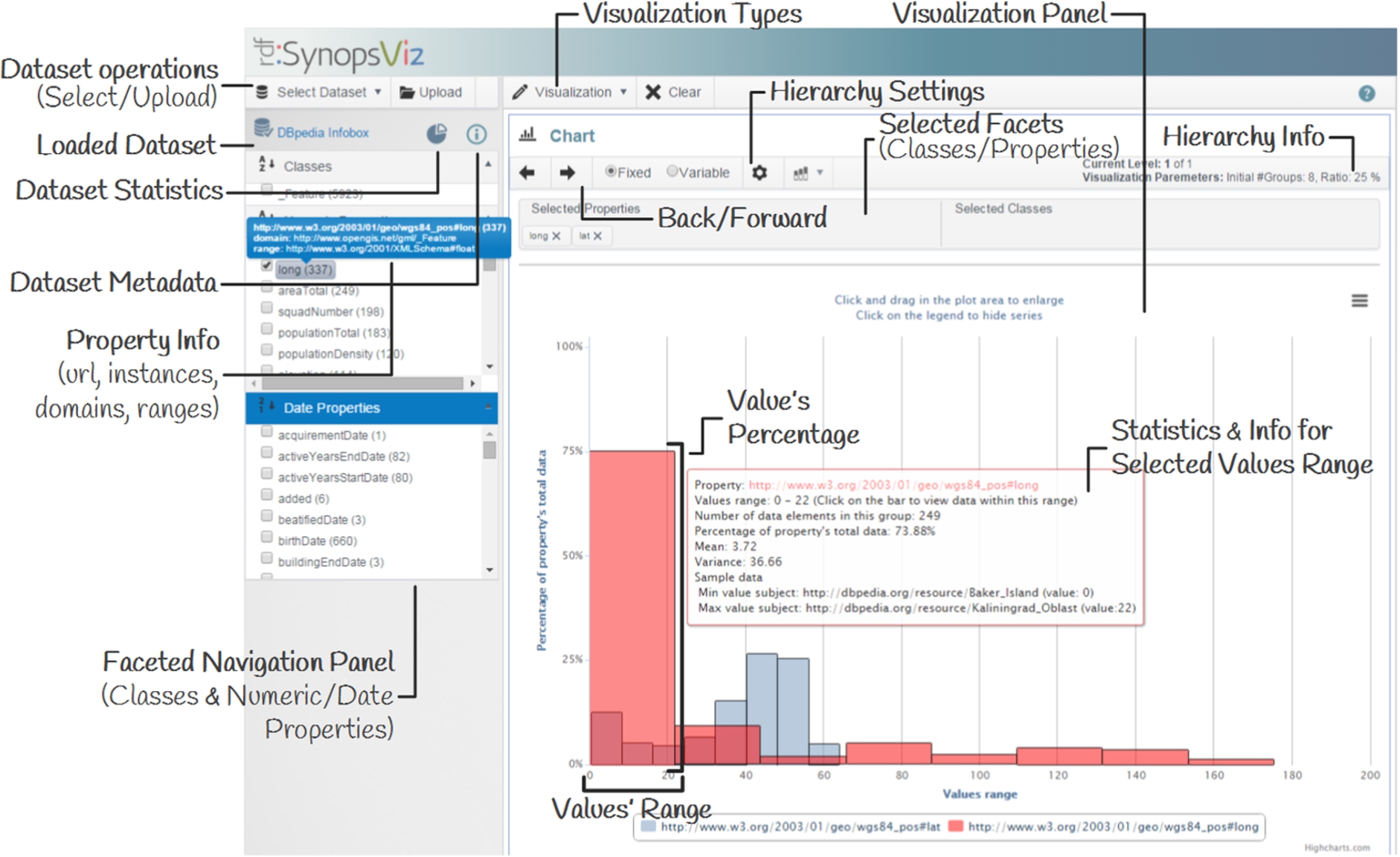
System architecture.

4. The SynopsViz tool

Based on the proposed hierarchical model, we have developed a web-based prototype called SynopsViz.13

¹³

synopsviz.imis.athena-innovation.gr.

The key features of SynopsViz are summarized as follows: (1) It supports the aforementioned hierarchical model for RDF data visualization, browsing and analysis. (2) It offers automatic on-the-fly hierarchy construction, as well as user-defined hierarchy construction based on users’ preferences. (3) Provides faceted browsing and filtering over classes and properties. (4) Integrates statistics with visualization; visualizations have been enriched with useful statistics and data information. (5) Offers several visualization techniques (e.g., timeline, chart, treemap). (6) Provides a large number of dataset’s statistics regarding the: data-level (e.g., number of sameAs triples), schema-level (e.g., most common classes/properties), and structure level (e.g., entities with the larger in-degree). (7) Provides numerous metadata related to the dataset: licensing, provenance, linking, availability, undesirability, etc. The latter can be considered useful for assessing data quality [115].

In the rest of this section, Section 4.1 describes the system architecture, Section 4.2 demonstrates the basic functionality of the SynopsViz. Finally, Section 4.3 provides technical information about the implementation.

4.1. System architecture

The architecture of SynopsViz is presented in Fig. 8. Our scenario involves three main parts: the Client UI, the SynopsViz, and the Input data. The Client part, corresponds to the system’s front-end offering several functionalities to the end-users. For example, hierarchical visual exploration, facet search, etc. (see Section 4.2 for more details). SynopsViz consumes RDF data as Input data; optionally, OWL-RDF/S vocabularies/ontologies describing the input data can be loaded. Next, we describe the basic components of the SynopsViz.

In the preprocessing phase, the Data and Schema Handler parses the input data and inferes schema information (e.g., properties domain(s)/range(s), class/ property hierarchy, type of instances, type of properties, etc.). Facet Generator generates class and property facets over input data. Statistics Generator computes several statistics regarding the schema, instances and graph structure of the input dataset. Metadata Extractor collects dataset metadata. Note that the model construction does not require any preprocessing, it is performed online, according to user interaction.

During runtime the following components are involved. Hierarchy Specifier is responsible for managing the configuration parameters of our hierarchy model, e.g., the number of hierarchy levels, the number of nodes per level, and providing this information to the Hierarchy Constructor. Hierarchy Constructor implements our tree structure. Based on the selected facets, and the hierarchy configuration, it determines the hierarchy of groups and the contained triples. Statistics Processor computes statistics about the groups included in the hierarchy. Visualization Module allows the interaction between the user and the back-end, allowing several operations (e.g., navigation, filtering, hierarchy specification) over the visualized data. Finally, the Hierarchical Model Module maintains the in-memory tree structure for our model and communicates with the Hierarchy Constructor for the model construction, the Hierarchy Specifier for the model customization, the Statistics Processor for the statistics computations, and the Visualization Module for the visual representation of the model.

Fig. 9.

Web user interface.

4.2. SynopsViz in-use

In this section we outline the basic functionality of SynopsViz prototype. Figure 9 presents the web user interface of the main window. SynopsViz UI consists of the following main panels: Facets panel: presents and manages facets on classes and properties; Input data control panel: enables the user to import and manage input datasets; Visualization panel: is the main area where interactive charts and statistics are presented; Configuration panel: handles visualization settings.

Initially, users are able to select a dataset from a number of offered real-word LD datasets (e.g., DBpedia, Eurostat) or upload their own. Then, for the selected dataset, the users are able to examine several of the dataset’s metadata, and explore several datasets’s statistics.

Using the facets panel, users are able to navigate and filter data based on classes, numeric and date properties. In addition, through facets panel several information about the classes and properties (e.g., number of instances, domain(s), range(s), IRI, etc.) are provided to the users through the UI.

Users are able to visually explore data by considering properties’ values. Particularly, area charts and timeline-based area charts are used to visualize the resources considering the user’s selected properties. Classes’ facets can also be used to filter the visualized data. Initially, the top level of the hierarchy is presented providing an overview of the data, organized into top-level groups; the user can interactively drill-down (i.e., zoom-in) and roll-up (i.e., zoom-out) over the group of interest, up to the actual values of the input data (i.e., LD resources). At the same time, statistical information concerning the hierarchy groups as well as their contents (e.g., mean value, variance, sample data, range) is presented through the UI (Fig. 10). Regarding the most detailed level (i.e., LD resources), several visualization types are offered; i.e., area, column, line, spline and areaspline (Fig. 10).

In addition, users are able to visually explore data, through class hierarchy. Selecting one or more classes, users can interactively navigate over the class hierarchy using treemaps (Fig. 10) or pie charts (Fig. 10). Properties’ facets can also be used to filter the visualized data. In SynopsViz the treemap visualization has been enriched with schema and statistical information. For each class, schema metadata (e.g., number of instances, subclasses, datatype/object properties) and statistical information (e.g., the cardinality of each property, min, max value for datatype properties) are provided.

Finally, users can interactively modify the hierarchy specifications. Particularly, they are able to increase or decrease the level of abstraction/detail presented, by modifying both the number of hierarchy levels, and number of nodes per level.

A video presenting the basic functionality of our prototype is available at youtu.be/n2ctdH5PKA0. Also, a demonstration of SynopsViz tool is presented in [19].

4.3. Implementation

SynopsViz is implemented on top of several open source tools and libraries. The back-end of our system is developed in Java, Jena framework is used for RDF data handing and Jena TDB is used for disk-based RDF storing. The front-end prototype, is developed using HTML and Javascript. Regarding visualization libraries, we use Highcharts, for the area, column, line, spline, areaspline and timeline-based charts and Google Charts for treemap and pie charts.

Fig. 10.

Numeric data & class hierarchy visualization examples.

5. Experimental analysis

In this section we present the evaluation of our approach. In Section 5.1, we present the dataset and the experimental setting. Then, in Section 5.2 we present the performance results and in Section 5.3 the user evaluation we performed.

5.1. Experimental setting

In our evaluation, we use the well known DBpedia 2014 LD dataset. Particularly, we use the Mapping-based Properties (cleaned) dataset14

¹⁴

downloads.dbpedia.org/2014/en/mappingbased_properties_cleaned_en.nt.bz2.

which contains high-quality data, extracted from Wikipedia Infoboxes. This dataset contains 33.1M triples and includes a large number of numeric and temporal properties of varying sizes. The largest numeric property in this dataset has 534K triples, whereas the largest temporal property has 762K.

Regarding the methods used in our evaluation, we consider our HETree hierarchical approaches, as well as a simple non-hierarchical visualization approach, referred as FLAT. FLAT is considered as a competitive method against our hierarchical approaches. It provides single-level visualizations, rendering only the actual data objects; i.e., it is the same as the visualization provided by SynopsViz at the most detailed level. In more detail, the FLAT approach corresponds to a column chart in which the resources are sorted in ascending order based on their object values, the horizontal axis contains the resources’ names (i.e., triples’ subjects), and the vertical axis corresponds to objects’ values. By hovering over a resource, a tooltip appears including the resource’s name and object value.

Regarding the HETree approaches, the tree parameters (i.e., number of leaves, degree and height) are automatically computed following the approach described in Section 2.5. In our experiments, the lower and the upper bound for the objects rendered at the most detailed level have been set to ${\mathit{\lambda }}_{\mathit{min}}=10$ and ${\mathit{\lambda }}_{\mathit{max}}=50$ , respectively. Considering the visualizations provided by the default Highcharts settings, these numbers are reasonable for our screen size and resolution.

Finally, our backend system is hosted on a server with a quad-core CPU at 2 GHz and 8 GB of RAM running Windows Server 2008. As client, we used a laptop with i5 CPU at 2.5 GHz with 4 G RAM, running Windows 7, Firefox 38.0.1 and ADSL2+ internet connection. Additionally, in the user evaluation, the client is employed with a 24” ( $1920\times 1200$ ) screen.

5.2. Performance evaluation

In this section, we study the performance of the proposed model, as well as the behaviour of our tool, in terms of construction and response time, respectively. Section 5.2.1 describes the setting of our performance evaluation, and Section 5.2.2 presents the evaluation results.

5.2.1. Setup

In order to study the performance, a number of numeric and temporal properties from the employed dataset are visualized using the two hierarchical approaches (i.e., HETree-C/R), as well as the FLAT approach. We select one set from each type of properties; each set contains 15 properties with varying sizes, starting from small properties having 50–100 triples up to the largest properties.

In our experiment, for each of the three approaches, we measure the tool response time. Additionally, for the two hierarchical approaches we also measure the time required for the HETree construction.

Note that in hierarchical approaches through user interaction, the server sends to the browser only the data required for rendering the current visualization level (although the whole tree is constructed at the backend). Hence, when a user requests to generate a visualization we have the following workflow. Initially, our system constructs the tree. Then, the data regarding the top-level groups (i.e., root node children) are sent to the browser which renders the result. Afterwards, based on user interactions (i.e., drill-down, roll-up), the server retrieves the required data from the tree and sends it to the browser. Thus, the tree is constructed the first time a visualization is requested for the given input dataset; for any further user navigation over the hierarchy, the response time does not include the construction time. Therefore, in our experiments, in the hierarchical approaches, as response time we measure the time required by our tool to provide the first response (i.e., render the top-level groups), which corresponds to the slower response in our visual exploration scenario. Thus, we consider the following measures in our experiments:

Construction Time: the time required to build the HETree structure. This time includes (1) the time for sorting the triples; (2) the time for building the tree; and (3) the time for the statistics computations.

Response Time: the time required to render the charts, starting from the time the client sends the request. This time includes (1) the time required by the server to compute and build the response. In the hierarchical approaches, this time corresponds to the Construction Time, plus the time required by the server to build the JSON object sent to the client. In the FLAT approach, it corresponds to the time spent in sorting the triples plus the time for the JSON construction; (2) the time spent in the client-sever communication; and (3) the time required by the visualization library to render the charts on the browser.

Table 4

Performance Results for Numeric & Temporal Properties

5.2.2. Results

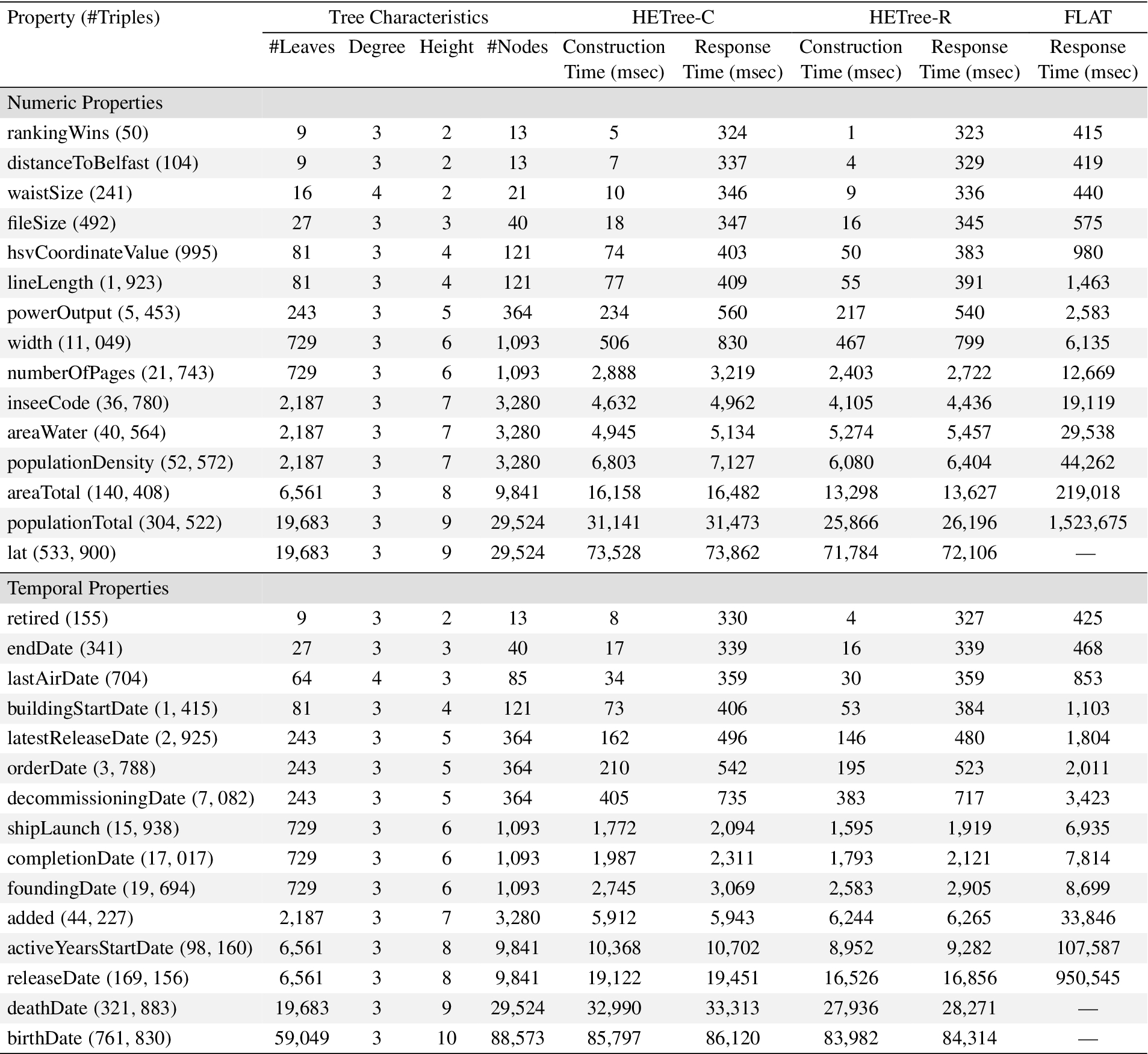
Table 4 presents the evaluation results regarding the numeric (upper half) and the temporal properties (lower half). The properties are sorted in ascending order of the number of triples. For each property, the table contains the number of triples, the characteristics of the constructed HETree structures (i.e., number of leaves, degree, height, and number of nodes), as well as the construction and the response time for each approach. The presented time measurements are the average values from 50 executions.

Regarding the comparison between the HETree and FLAT, the FLAT approach can not provide results for properties having more than 305K triples, indicated in the last rows for both numeric and temporal properties with “—” in the FLAT response time. For the rest properties, we can observe that the HETree approaches clearly outperform FLAT in all cases, even in the smallest property (i.e., rankingWin, 50 triples). As the size of properties increases, the difference between the HETree approaches and FLAT increases, as well. In more detail, for large properties having more than 53K triples (i.e., the numeric properties larger than the populationDensity -12th row-, and the temporal properties larger than the added -11th row-), the HETree approaches outperform the FLAT by one order of magnitude.

Regarding the time required for the construction of the HETree structure, from Table 4 we can observe the following: The performance of both HETtree structures is very close for most of the examined properties, with the HETree-R performing slightly better than the HETree-C (especially in the relatively small numeric properties). Furthermore, we can observe that the response time follows a similar trend as the construction time. This is expected since the communication cost, as well as the times required for constructing and rendering the JSON object are almost the same for all cases.

Regarding the comparison between the construction and the response time in the HETree approaches, from Table 4 we can observe the following. For properties having up to 5.5K triples (i.e., the numeric properties smaller than the width -8th row-, and the temporal properties smaller than the decommissioningDate -7th row-), the response time is dominated by the communication cost, and the time required for the JSON construction and rendering. For properties with only a small number of triples (i.e., waistSize, 241 triples), only 1.5% of the response time is spent on constructing the HETree. Moreover, for a property with a larger number of triples (i.e., buildingStartData, 1.415 triples), 18% of the time is spent on constructing the HETree. Finally, for the largest property for which the time spent in communication cost, JSON construction and rendering is larger than the construction time (i.e., powerOutput, 5.453 triples), 42% of the time is spent on constructing the HETree.

Fig. 11.

Response Time w.r.t. the number of triples.

Figure 11 summarizes the results from Table 4, presenting the response time for all approaches w.r.t. the number of triples. Particularly, Fig. 11(a) includes all properties sizes (i.e., 50 to 762K). Further, in order to have a precise observation over small property sizes (Small properties) in which the difference between the FLAT and the HETree approaches is smaller, we report properties with less than 20K triples separately in Fig. 11(b). Once again, we observe that HETree-R performs slightly better than the HETree-C. Additionally, from Fig. 11(b) we can indicate that for up to 10K triples the performance of the HETree approaches is almost the same. We can also observe the significant difference between the FLAT and the HETree approaches.

However our method clearly outperforms the non-hierarchical method, as we can observe from the above results, the construction of the whole hierarchy can not provide an efficient solution for datasets containing more than 10K objects. As discussed in Section 3.2, for efficient exploration over large datasets an incremental hierarchy construction is required. In the incremental exploration scenario, the number of hierarchy nodes that have to be processed and constructed is significantly fewer compared to the non-incremental.

For example, adopting an non-incremental construction in populationTotal (305K triples), 29.6K nodes are to be initially constructed (along with their statistics). On the other hand, with the incremental approach (as analysed in Section 3.2) at the beginning of each exploration scenario, only the initial nodes are constructed. Initial nodes are the nodes initially presented, as well as the nodes potentially reached by the user’s first operation.

In the RES scenario, the initial nodes are the leaf of interest (1 node) and its sibling leaves (at most $\mathit{d}-1$ nodes). In the RAN, the initial nodes are the nodes of interest (at most d nodes), their children (at most ${\mathit{d}}^2$ nodes), and their parent node along with its siblings (at most d nodes). Finally, in the BSC scenario the initial nodes are the root node (1 node) and its children (at most d nodes). Overall, at most d, $2\mathit{d}+{\mathit{d}}^2$ , and $\mathit{d}+1$ nodes are initially constructed in the RES, RAN, and BSC scenarios respectively. Therefore, in populationTotal case where $\mathit{d}=3$ at most 3, 15 and 4 nodes are initially constructed in the RES, RAN, and BSC scenarios respectively.

5.3. User study

In this section we present the user evaluation of our tool, where we have employed three approaches: the two hierarchical and the FLAT. Section 5.3.1 describes the user tasks, Section 5.3.2 outlines the evaluation procedure and setup, Section 5.3.3 summarizes the evaluation results, and Section 5.3.4 discusses issues related to the evaluation process.

5.3.1. Tasks

In this section we describe the different types of tasks that are used in the user evaluation process.

Type 1 [Find resources with specific value]: This type of tasks requests the resources having value v (as object). For this task type, we define task T1 by selecting a value v that corresponds to 5 resources. Given this task, the participants are asked to provide the number of resources that pertain to this value. In order to solve this task, the participants first have to find a resource with value v and then check which of the nearby resources also have the same value.

Type 2 [Find resources in a range of values]: This type of tasks requests the resources having value greater than ${\mathit{v}}_{\mathit{min}}$ and less than ${\mathit{v}}_{\mathit{max}}$ . We define two tasks of this type, by selecting different combinations of ${\mathit{v}}_{\mathit{min}}$ and ${\mathit{v}}_{\mathit{max}}$ values, such that tasks which consider different numbers of resources are defined. We define two tasks, the first task considers a relative small number of resources while the second a larger. In our experiments we select 10 as a small number of resources, while as a large number we select 50. Particularly, in the first task, named T2.1, we specify the values ${\mathit{v}}_{\mathit{min}}$ and ${\mathit{v}}_{\mathit{max}}$ such that a relatively small set of (approximately 10) resources are included, whereas the second task, T2.2, considers a relatively larger set of (approximately 50) resources. Given these tasks, the participants are asked to provide the number of resources included in the given range. This task can be solved by first finding a resource with a value included in the given range, and then explore the nearby resources in order to identify the resources in the given range.

Type 3 [Compare distributions]: This type of tasks requests from the participant to identify whether more resources appear above or below a given value v. For this type, we define task T3, by selecting the value v near to the median. Given this task, the participants are asked to provide the number of resources appearing either above or below the value v. The answer for this tasks requires from the participants to indicate the value v and determine the number or resources appearing either before or after this value.

Table 5

Average Task Completion Time (sec)

	Small Property				Large Property
	FLAT	HETree-C	HETree-R	p	FLAT	HETree-C	HETree-R	p
T1	54	29	28		85	52	47
T2.1	63	57	64		74	60	69
T2.2	120	69	74		128	72	77
T3	262	41	40		—	64	62	—

  $\mathrm{(}\mathit{p}\mathrm{<}0.01\mathrm{)}$    $\mathrm{(}\mathit{p}\mathrm{<}0.05\mathrm{)}$    $\mathrm{(}\mathit{p}\mathrm{>}0.05\mathrm{)}$

Table 6

Error Rate (%)

	Small Property				Large Property
	FLAT	HETree-C	HETree-R	p	FLAT	HETree-C	HETree-R	p
T1	0	0	0		0	0	0
T2.1	0	0	0		0	0	0
T2.2	20	0	0		20	0	10
T3	70	0	0		—	0	0	—

  $\mathrm{(}\mathit{p}\mathrm{<}0.01\mathrm{)}$    $\mathrm{(}\mathit{p}\mathrm{<}0.05\mathrm{)}$    $\mathrm{(}\mathit{p}\mathrm{>}0.05\mathrm{)}$

5.3.2. Setup

In order to study the effect of the property size in the selected tasks, we have selected two properties of different sizes from the employed dataset (Section 5.1). The hsvCoordinateHue numeric property containing 970 triples, is referred to as Small, and the maximumElevation numeric property, containing 37.936 triples, is referred to as Large. The first one corresponds to a hierarchy of height 4 and degree 3, and the latter corresponds to a hierarchy of height 7 and degree 3. We should note here that through the user evaluation, the hierarchy parameters were fixed for all the tasks, and the participants were not allowed to modify them, such that the setting has been the same for everyone.

In our evaluation, 10 participants took part. The participants were computer science graduate students and researchers. At the beginning of the evaluation, each participant has introduced to the system by an instructor who provided a brief tutorial over the features required for the tasks. After the instructions, the participants familiarized themselves with the system. Note that we have integrated in the SynopsViz the FLAT approach along with the HETree approaches.

During the evaluation, each participant performed the previously described four tasks, using all approaches (i.e., HETree-C/R and FLAT), over both the small and large properties. In order to reduce the learning effects and fatigue we defined three groups. In the first group, the participants start their tasks with the HETree-C approach, in the second with HETree-R, and in the third with FLAT. Finally, the property (i.e., small, large) first used in each task was counterbalanced among the participants and the tasks. The entire evaluation did not exceed 75 minutes.

Furthermore, for each task (e.g., T2.1, T.3), three task instances were specified by slightly modifying the task parameters. As a result, given a task, a participant has to solve a different instance of this task, in each approach.

For example, in task T2.1, for the HETree-R, the selected v corresponds to a solution of 11 resources, in HETree-C, to 9 resources, whereas for FLAT v corresponded to a solution of 8 resources. The task instance assigned to each approach varied among the participants.

During the evaluation the instructor measured the time required for each participant to complete a task, as well as the number of incorrect answers. Table 5 presents the average time required for the participants to complete each task. The table contains the measurements for all approaches, and for both properties. Although we acknowledge that the number of participants in our evaluation is small, we have computed the statistical significance of the results. Essentially, for each property, the p-value of each task is presented in the last column. The p-value is computed using one-way repeated measures ANOVA.

In addition, the results regarding the number of tasks that were not correctly answered are presented in Table 6. Particularly, the table presents the percentage of incorrect answers for each task and property, referred to as error rate. Additionally, for each task and property, the table includes the p-value. Here, the p-value has been computed using Fisher’s exact test.

5.3.3. Results

Task T1. Regarding the first task, as we can observe from Table 5, the HETree approaches outperform FLAT, in both property sizes. Note that the time results on T1 are statistically significant ( $\mathit{p}\mathrm{<}0.01$ ).

As expected, all approaches require more time for the Large property compared to the Small one. This overhead in FLAT is caused by the larger number of resources that the participants have to scroll over and examine, until they indicate the requested resource’s value. On the other hand, in HETree, the overhead is caused by the larger number of levels that the Large property hierarchy has. Hence, the participants have to perform more drill-down operations and examine more groups of objects, until they reach the LD resources.

We can also observe that in this task, the HETree-R performs slightly better than the HETree-C in both property sizes. This is due to the fact that, in HETree-R structure, resources having the same value are always contained in the same leaf. As a result, the participants had to inspect only one leaf. On the other hand, in HETree-C this does not always hold, hence the participants could have explored more than one leaf.

Finally, as we can observe from Table 6, in all cases only correct answers have been provided. However, none of those results are statistically significant ( $\mathit{p}\mathrm{>}0.05$ ).

Task T2.1. In the next task, where the participants had to indicate a small set of resources in a range of values, the FLAT performance is very close to the HETree, especially in the Small property (Table 5). In addition, we can observe that the HETree-C approach performs slightly better than the HETree-R. Finally, regarding the statistical significance of the results, in Small property we have $\mathit{p}\mathrm{>}0.05$ , while in Large we have $\mathit{p}\mathrm{<}0.005$ .

The poor performance of the HETree approaches in this task can be explained by the small set of resources requested and the HETree parameters adopted in the user evaluation. In this setting, the resources contained in the task solution are distributed over more than one leaves. Hence, the participants had to perform several roll-up and drill-down operations in order to find all the resources. On the other hand, in FLAT, once the participants had indicated one of the requested resources, it was very easy for them to find out the rest of the solution’s resources. To sum up, in FLAT, most of the time is spent on identifying the first of the resources, while in HETree the first resource is identified very quickly. Regarding the difference in performance between the HETree approaches we have the following. In HETree-C due to the fixed number of objects in each leaf, the participants had to visit at most one or two leaves in order to solve this task. On the other hand, in HETree-R, the number of objects in each leaf is varied, so most times the participants had to inspect more than two leaves in order to solve the task. Finally, also in this case only correct answers were given (Table 6).

Task T2.2. In this task the participants had to indicate a larger set (compared to the previous task) of resources given a range of values. HETree approaches noticeably outperform the FLAT approach with statistical significance ( $\mathit{p}\mathrm{<}0.01$ ), while similar results are observed in both properties.

In the FLAT approach a considerable time was spent to identify and navigate over a large number of resources. On the other hand, due to the large number of resources involved in the task’s solution, there are groups in the hierarchy that explicitly contain resources of solutions (i.e., they do not contain resources not included in the solution). As a result, the participants in HETree could easily indicate and compute the whole solution by combining the information related to the groups (i.e., number of enclosed resources) and individual resources. Due to the same reasons stated in the previous task (i.e., T2.1), similarly in T2.2 the HETree-C performs slightly better than the HETree-R. Finally, we can observe from Table 6 (but without statistical significance), that it was more difficult for participants to solve correctly this task with FLAT than with HETree.

Task T3. In the last task, participants were requested to find which of the two ranges contained more resources. As expected, Table 5 shows that the HETree approaches clearly outperform the FLAT approach with statistical significance in the Small property. This is due to the fact that the participants in FLAT had to overview and navigate over almost half of the dataset. As a result, apart from the long time required for this process, it was also very difficult to find the correct solution. This is also verified by Table 6 on a statistically significant level. On the other hand, in the HETree approaches, the participants could easily find out the answer by considering the resources enclosed by several groups.

Regarding the Large property, as it is expected, it was impossible for participants to solve this task with FLAT, since this required to parse over and count about 19K resources. As a result, none of the participants completed this task using FLAT (indicated with “—” in Table 5), considering the 5 minute time limit used in this task.

5.3.4. Discussion

The user evaluation showed that the hierarchical approaches can be efficient (i.e., require short time in solving tasks) and effective (i.e., have lower error rate) in several cases. In more detail, the HETree approaches performed very well on indicating specific values over a dataset, and given the appropriate parameter setting are marginally affected by the dataset size. Also note that due to the “vertical-based” exploration, the position (e.g., towards the end) of the requested value in the dataset does not affect the efficiency of the approach. Furthermore, it is shown that the hierarchical approaches can efficiently and effectively handle visual exploration tasks that involve large numbers of objects.

At the end of the evaluation, the participants gave us valuable feedbacks on possible improvements of our tool. Most of the participants criticized several aspects in the interface, since our tool is an early prototype. Also, several participants mentioned difficulties in obtaining their “position” (e.g., which is the currently visualized range of values, or the previously visualized range of values) during the exploration. Finally, some participants mentioned that some hierarchies contained more levels than needed. As previously mentioned, the adopted parameters are not well suited for the evaluation, since hierarchies with a degree larger than 3 (and as result less levels) are required.

Finally, additional tasks for demonstrating the capabilities of our model can be considered. However, most of these tasks were not selected in this evaluation, because it was not possible for the participants to perform them with the FLAT approach. An indicative set includes: (1) Find the number of resources (and/or statistics) in the 1st and 3rd quartile; (2) Find statistics (e.g., mean value, variance) for the top-10 or 50 resources; (3) Find the decade (i.e., temporal data) in which most events take place.

Table 7

Visualization Systems Overview

6. Related work

This section reviews works related to our approach on visualization and exploration in the Web of Data (WoD). Section 6.1 presents systems and techniques for WoD visualization and exploration, Section 6.2 discusses techniques on WoD statistical analysis, Section 6.3 present hierarchical data visualization techniques, and finally, Section 6.4 discusses works on data structures & processing related to our HETree data structure.

In Table 7 we provide an overview and compare several visualization systems that offer similar features to our SynopsViz. The WoD column indicates systems that target the Semantic Web and Linked Data area (i.e., RDF, RDF/S, OWL). The Hierarchical column indicates systems that provide hierarchical visualization of non-hierarchical data. The Statistics column captures the provision of statistics about the visualized data. The Recomm. column indicates systems, which offer recommendation mechanisms for visualization settings (e.g., appropriate visualization type, visualization parameters, etc.). The Incr. column indicate systems that provide incremental visualizations. Finally, the Preferences column captures the ability of the users to apply data (e.g., aggregate) or visual (e.g., increase abstraction) operations.

6.1. Exploration & visualization in the Web of Data

A large number of works studying issues related to WoD visual exploration and analysis have been proposed in the literature [3,18,30,79]. In what follows, we classify these works into the following categories: (1) Generic visualization systems, (2) Domain, vocabulary & device-specific visualization systems, and (3) Graph-based visualization systems.

6.1.1. Generic visualization systems

In the context of WoD visual exploration, there is a large number of generic visualization frameworks, that offer a wide range of visualization types and operations. Next, we outline the best known systems in this category.

Rhizomer [21] provides WoD exploration based on a overview, zoom and filter workflow. Rhizomer offers various types of visualizations such as maps, timelines, treemaps and charts. VizBoard [109,110] is an information visualization workbench for WoD build on top of a mashup platform. VizBoard presents datasets in a dashboard-like, composite, and interactive visualization. Additionally, the system provides visualization recommendations. Payola [67] is a generic framework for WoD visualization and analysis. The framework offers a variety of domain-specific (e.g., public procurement) analysis plugins (i.e., analyzers), as well as several visualization techniques (e.g., graphs, tables, etc.). In addition, Payola offers collaborative features for users to create and share analyzers. In Payola the visualizations can be customized according to ontologies used in the resulting data.

The Linked Data Visualization Model (LDVM) [20] provides an abstract visualization process for WoD datasets. LDVM enables the connection of different datasets with various kinds of visualizations in a dynamic way. The visualization process follows a four stage workflow: Source data, Analytical abstraction, Visualization abstraction, and View. A prototype based on LDVM considers several visualization techniques, e.g., circle, sunburst, treemap, etc. Finally, the LDVM has been adopted in several use cases [68]. Vis Wizard [105] is a Web-based visualization system, which exploits data semantics to simplify the process of setting up visualizations. Vis Wizard is able to analyse multiple datasets using brushing and linking methods. Similarly, Linked Data Visualization Wizard (LDVizWiz) [6] provides a semi-automatic way for the production of possible visualization for WoD datasets. In a same context, LinkDaViz [103] finds the suitable visualizations for a give part of a dataset. The framework uses heuristic data analysis and a visualization model in order to facilitate automatic binding between data and visualization options.

Balloon Synopsis [91] provides a WoD visualizer based on HTML and JavaScript. It adopts a node-centric visualization approach in a tile design. Additionally, it supports automatic information enhancement of the local RDF data by accessing either remote SPARQL endpoints or performing federated queries over endpoints using the Balloon Fusion service. Balloon Synopsis offers customizable filters, namely ontology templates, for the users to handle and transform (e.g., filter, merge) input data. SemLens [51] is a visual system that combines scatter plots and semantic lenses, offering visual discovery of correlations and patterns in data. Objects are arranged in a scatter plot and are analysed using user-defined semantic lenses. LODeX [15] is a system that generates a representative summary of a WoD source. The system takes as input a SPARQL endpoint and generates a visual (graph-based) summary of the WoD source, accompanied by statistical and structural information of the source. LODWheel [99] is a Web-based visualizing system which combines JavaScript libraries (e.g., MooWheel, JQPlot) in order to visualize RDF data in charts and graphs. Hide the stack [31] proposes an approach for visualizing WoD for mainstream end-users. Underlying Semantic Web technologies (e.g., RDF, SPARQL) are utilized, but are “hidden” from the end-users. Particularly, a template-based visualization approach is adopted, where the information for each resource is presented based on its rdf:type.

6.1.2. Domain, vocabulary & device-specific visualization systems

In this section, we present systems that target visualization needs for specific types of data and domains, RDF vocabularies or devices.

Several systems focus on visualizing and exploring geo-spatial data. Map4rdf [73] is a faceted browsing tool that enables RDF datasets to be visualized on an OSM or Google Map. Facete [97] is an exploration and visualization system for SPARQL accessible data, offering faceted filtering functionalities. SexTant [81] and Spacetime [107] focus on visualizing and exploring time-evolving geo-spatial data. The LinkedGeoData Browser [96] is a faceted browser and editor which is developed in the context of LinkedGeoData project. Finally, in the same context DBpedia Atlas [106] offers exploration over the DBpedia dataset by exploiting the dataset’s spatial data. Furthermore, in the context of linked university data, VISUalization Playground (VISU) [4] is an interactive tool for specifying and creating visualizations using the contents of linked university data cloud. Particularly, VISU offers a novel SPARQL interface for creating data visualizations. Query results from selected SPARQL endpoints are visualized with Google Charts.

A variety of systems target multidimensional WoD modelled with the Data Cube vocabulary. CubeViz [37,90] is a faceted browser for exploring statistical data. The system provides data visualizations using different types of charts (i.e., line, bar, column, area and pie). The Payola Data Cube Vocabulary [52] adopts the LDVM stages [20] in order to visualize RDF data described by the Data Cube vocabulary. The same types of charts as in CubeViz are provided in this system. The OpenCube Toolkit [59] offers several systems related to statistical WoD. For example, OpenCube Browser explores RDF data cubes by presenting a two-dimensional table. Additionally, the OpenCube Map View offers interactive map-based visualizations of RDF data cubes based on their geo-spatial dimension. The Linked Data Cubes Explorer (LDCE) [63] allows users to explore and analyse statistical datasets. Finally, [84] offers several map and chart visualizations of demographic, social and statistical linked cube data.15

¹⁵

www.linked-statistics.gr.

Regarding device-specific systems, DBpedia Mobile [14] is a location-aware mobile application for exploring and visualizing DBpedia resources. Who’s Who [23] is an application for exploring and visualizing information focusing on several issues that appear in the mobile environment. For example, the application considers the usability and data processing challenges related to the small display size and limited resources of the mobile devices.

6.1.3. Graph-based visualization systems

A large number of systems visualize WoD datasets adopting a graph-based (a.k.a., node-link) approach. RelFinder [50] is a Web-based tool that offers interactive discovery and visualization of relationships (i.e., connections) between selected WoD resources. Fenfire [48] and Lodlive [22] are exploratory systems that allow users to browse WoD using interactive graphs. Starting from a given URI, the user can explore WoD by following the links. IsaViz [86] allows users to zoom and navigate over the RDF graph, and also it offers several “edit” operations (e.g., delete/add/rename nodes and edges). In the same context, graphVizdb [16,17] is built on top of spatial and database techniques offering interactive visualization over very large (RDF) graphs. A different approach has been adopted in [100], where sampling techniques have been exploited. Finally, ZoomRDF [116] employs a space-optimized visualization algorithm in order to increase the number of resources which are displayed.

6.1.4. Discussion

In contrast to the aforementioned approaches, our work does not focus solely on proposing techniques for WoD visualization. Instead, we introduce a generic model for organizing, exploring and analysing numeric and temporal data in a multilevel fashion. The underlying model is not bound to any specific type of visualization (e.g., chart); rather it can be adopted by several “flat” techniques and offer multilevel visualizations over non-hierarchical data. Also, we present a prototype system that employs the introduced hierarchical model and offers efficient multilevel visual exploration over WoD datasets, using charts and timelines.

6.2. Statistical analysis in the Web of Data

A second area related to the analysis features of the proposed model deals with WoD statistical analysis. RDFStats [71] calculates statistical information about RDF datasets. LODstats [9] is an extensible framework, offering scalable statistical analysis of WoD datasets. RapidMiner LOD Extension [83,87] is an extension of the data mining platform RapidMiner,16

¹⁶

rapidminer.com.

offering sophisticated data analysis operations over WoD. SparqlR17

¹⁷

cran.r-project.org/web/packages/SPARQL/index.html.

is a package of the R18

¹⁸

www.r-project.org.

statistical analysis platform. SparqlR executes SPARQL queries over SPARQL endpoints and provides statistical analysis and visualization over SPARQL results. Finally, ViCoMap [88] combines WoD statistical analysis and visualization, in a Web-based tool, which offers correlation analysis and data visualization on maps.

6.2.1. Discussion

In comparison with these systems, our work does not focus on new techniques for WoD statistics computation and analysis. We are primarily interested on enhancing the visualization and user exploration functionality by providing statistical properties of the visualized datasets and objects, making use of existing computation techniques. Also, we demonstrate how in the proposed structure, computations can be efficiently performed on-the-fly and enrich our hierarchical model. The presence of statistics provides quantifiable overviews of the underlying WoD resources at each exploration step. This is particularly important in several tasks when you have to explore a large number of either numeric or temporal data objects. Users can examine next levels’ characteristics at a glance, this way are not enforced to drill down in lower hierarchy levels. Finally, the statistics over the different hierarchy levels enables analysis over different granularity levels.

6.3. Hierarchical visual exploration

The wider area of data and information visualization has provided a variety of approaches for hierarchical analysis and presentation.

Treemaps [93] visualize tree structures using a space-filling layout algorithm based on recursive subdivision of space. Rectangles are used to represent tree nodes, the size of each node is proportional to the cumulative size of its descendant nodes. Finally, a large number of treemaps variations have been proposed (e.g., Cushion Treemaps, Squarified Treemaps, Ordered Treemaps, etc.).

Moreover, hierarchical visualization techniques have been extensively employed to visualize very large graphs using the node-link paradigm. In these techniques the graph is recursively decomposed into smaller sub-graphs that form a hierarchy of abstraction layers. In most cases, the hierarchy is constructed by exploiting clustering and partitioning methods [1,7,11,74,89,104]. In other works, the hierarchy is defined with hub-based [75] and density-based [117] techniques. GrouseFlocks [5] supports ad-hoc hierarchies which are manually defined by the users. Finally, there also some edge bundling techniques which join graph edges to bundles. The edges are often aggregated based on clustering techniques [38,41,85], a mesh [28,70] or explicitly by a hierarchy [53].

In the context of data warehousing and online analytical processing (OLAP), several approaches provide hierarchical visual exploration, by exploiting the predefined hierarchies in the dimension space. [78] proposes a class of OLAP-aware hierarchical visual layouts; similarly, [102] uses OLAP-based hierarchical stacked bars. Polaris [98] offers visual exploratory analysis of data warehouses with rich hierarchical structure.

Several hierarchical techniques have been proposed in the context of ontology visualization and exploration [34,40,46,72]. CropCircles [111] adopts a hierarchical geometric containment approach, representing the class hierarchy as a set of concentric circles. Knoocks [69] combines containment-based and node-link approaches. In this work, ontologies are visualized as nested blocks where each block is depicted as a rectangle containing a sub-branch shown as tree map. A different approach is followed by OntoTrix [10] which combine graphs with adjacency matrices.

Finally, in the context of hierarchical navigation, [64] organizes query results using the MeSH concept hierarchy. In [24] a hierarchical structure is dynamically constructed to categorize numeric and categorical query results. Similarly, [26] constructs personalized hierarchies by considering diverse users preferences.

6.3.1. Discussion

In contrast to above approaches that target graph-based or hierarchically-organized data, our work focuses on handling arbitrary numeric and temporal data, with out requiring it to be described by an hierarchical schema. As an example of hierarchically-organized data, consider class hierarchies or multidimensional data organized in multilevel hierarchical dimensions (e.g., in OLAP context, temporal data is hierarchically organized based on years, months, etc.). In contrast to aforementioned approaches, our work dynamically constructs the hierarchies from raw numeric and temporal data. Thus the proposed model can be combined with “flat” visualization techniques (e.g., chart, timeline), in order to provide multilevel visualizations over non-hierarchical data. In that sense, our approach can be considered more flexible compared to the techniques that rely on predefined hierarchies, as it can enable exploratory functionality on dynamically retrieved datasets, by (incrementally) constructing hierarchies on-the-fly, and allowing users to modify these hierarchies.

6.4. Data structures & data processing

In this section we present the data structures and the data (pre-)processing techniques which are the most relevant to our approach.

R-Tree [45] is disk-based multi-dimensional indexing structure, which has been widely used in order to efficiently handle spatial queries. R-Tree adopts the notion of minimum bounding rectangles (MBRs) in order to hierarchical organize multi-dimensional objects.

Data discretization [33,42] is a process where continuous attributes are transformed into discrete. A large number of methods (e.g., supervised, unsupervised, univariate, multivariate) for data discretization have been proposed. Binning is a simple unsupervised discretization method in which a predefined number of bins is created. Widely known binning methods are the equal-width and equal-frequency. In equal-width approach, the range of an attribute is divided into intervals that have equal width and each interval represents a bin. In equal-frequency approach, an equal number of values are placed in each bin.

By recursively applying discretization techniques, a hierarchical discretization of attribute’s values can be produced (a.k.a. concept/generalization hierarchies). In [92] a dynamic programming algorithm for generating numeric concept hierarchies is proposed. The algorithm attempts to maximize both the similarity between the objects stored in the same hierarchy’s node, as well as the dissimilarity between the objects stored in different nodes. The generated hierarchy is a balanced tree where different nodes may have different number of children. Similarly, [47] constructs hierarchies based on data distribution. Essentially, both the leaf and the interval nodes are created in such a way that an even distribution is achieved. The hierarchy construction considers also a threshold specifying the maximum number of distinct values enclosed by nodes in each hierarchy level. Finally, binary concept hierarchies (with degree equal to two) are generated in [27]. Starting from the whole dataset, it performs a recursive binary partitioning over the dataset’s values; the recursion is terminated when the number of distinct values in the resultant partitions is less than a pre-specified threshold.

Using the data objects from our running example (Fig. 1), Fig. 12 shows the hierarchies generated from the aforementioned approaches. Figure 12(a) presents the hierarchy resulting from [27] and Fig. 12(b) depicts the result using the method from [47]. The parameters in each method are set, so that the resulting hierarchies are as much as possible similar to our hierarchies (Figs 2 and 3). Hence, the threshold in (a) is set to 3, and in (b) is set to 2.

6.4.1. Discussion

The basic concepts of HETree structure can be considered similar to a simplified version of a static 1D R-Tree. However, in order to provide efficient query processing in disk-based environment, R-Tree considers a large number of I/O-related issues (e.g., space coverage, nodes overlaps, fill guarantees, etc.). On the other hand, we introduce a lightweight, main memory structure that efficiently constructed on-the-fly. Also, the proposed structure aims at organizing the data in a practical manner for a (visual) exploration scenario, rather than for disk-based indexing and querying efficiency.

Compared to discretization techniques, our tree model exhibits several similarities, namely, the HETree-C version can be considered as a hierarchical version of the equal-frequency binning, and the HETree-R of the equal-width binning. However, the goal of data organization in HETree is to enable visualization and hierarchical exploration capabilities over dynamically retrieved non-hierarchical data. Hence, compared to the binning methods we can consider the following basic differences. First, in contrast with binning methods that require from the user to specify some parameters (e.g., the number/size of the bins, the number of distinct values in each bin, etc); our approach is able to automatically estimate the hierarchy parameters and adjust the visualization results by considering the visualization environment characteristics. Second, in hierarchical approaches the user is not always allowed to specify the hierarchy characteristics (e.g., degree). For example, the hierarchies in [27] have always degree equal to two (Fig. 12(a)), while in [47] the nodes have varying degrees (Fig. 12(b)). On the other hand, in our approach the hierarchy characteristics can be specified precisely. In addition, when not specific hierarchy characteristics are requested, our approach generates perfect trees (Section 2.5), offering a “uniform” hierarchy structure. Third, the computational complexity in some of the hierarchical approaches (e.g., [92]) is prohibitive (i.e., at least cubic) for using them in practise; especially in settings where the hierarchies have to constructed on-the-fly. Fourth, the proposed tree structure is exploited in order to allow efficient statistics computations over different groups of data; then, the statistics are used in order to enhance the overall exploration functionality. Finally, the construction of the model is tailored to the user interaction and preferences; our model offers incremental construction considering the user interaction, as well as efficiently adaptation to the users preferences.

Fig. 12.

Hierarchies generated from different approaches. a) based on [27] b) based on [47].

7. Conclusions

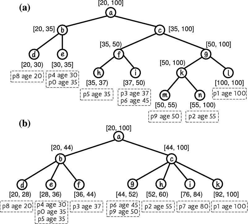
In this paper we have presented HETree, a generic model that combines personalized multilevel exploration with online analysis of numeric and temporal data. Our model is built on top of a lightweight tree-based structure, which can be efficiently constructed on-the-fly for a given set of data. We have presented two variations for constructing our model: the HETree-C structure organizes input data into fixed-size groups, whereas the HETree-R structure organizes input data into fixed-range groups. In that way, the users can customize the exploration experience, allowing them to organize data into different ways, by parameterizing the number of groups, the range and cardinality of their contents, the number of hierarchy levels, and so on. We have also provided a way for efficiently computing statistics over the tree, as well as a method for automatically deriving from the input dataset the best-fit parameters for the construction of the model. Regarding the performance of multilevel exploration over large datasets, our model offers incremental HETree construction and prefetching, as well as efficient HETree adaptation based on user preferences. Based on the introduced model, a Web-based prototype system, called SynopsViz, has been developed. Finally, the efficiency and the effectiveness of the presented approach are demonstrated via a thorough performance evaluation and an empirical user study.

Some insights for future work include the support of sophisticated methods for data organization in order to effectively handle skewed data distributions and outliers. Particularly, we are currently working on hybrid HETree versions, that integrate concepts from both HETree-C and HETree-R version. For example, a hybrid HETree-C considers a threshold regarding the maximum range of a group; similarly, a threshold regarding the maximum number of objects in a group is considered in hybrid HETree-R version. Regarding the SynopsViz tool, we are planning to redesign and extend the graphical user interface, so our tool to be able to use data resulting from SPARQL endpoints, as well as to offer more sophisticated filtering techniques (e.g., SPARQL-enabled browsing over the data). Finally, we are interested in including more visual techniques and libraries.