Sage Journals: Discover world-class research

Abstract

In this paper we present Spatial-KWD, a free open-source tool for efficient computation of the Kantorovich-Wasserstein Distance (KWD), also known as Earth Mover Distance, between pairs of binned spatial distributions (histograms) of a non-negative variable. KWD can be used in spatial statistics as a measure of (dis)similarity between spatial distributions of physical or social quantities. KWD represents the minimum total cost of moving the “mass” from one distribution to the other when the “cost” of moving a unit of mass is proportional to the euclidean distance between the source and destination bins. As such, KWD captures the degree of “horizontal displacement” between the two input distributions. Despite its mathematical properties and intuitive physical interpretation, KWD has found little application in spatial statistics until now, mainly due to the high computational complexity of previous implementations that did not allow its application to large problem instances of practical interest. Building upon recent advances in Optimal Transport theory, the Spatial-KWD library allows to compute KWD values for very large instances with hundreds of thousands or even millions of bins. Furthermore, the tool offers a rich set of options and features to enable the flexible use of KWD in diverse practical applications.

Keywords

Spatial distributions similarity measures wasserstein distance earth mover distance

1. Introduction

In several statistical domains that involve a spatial component it is often required to deal with measurements or estimates of physical or social quantities defined over a finite geographic region. In particular, we address in this contribution the case where (i) the target variable of interest to be measured or estimated is non-negative and (ii) the spatial domain is represented by a regular square grid. In such applications, the spatial distribution of the non-negative variable of interest is represented by a bi-dimensional histogram. A prominent example are census population grids.1

¹
Population and housing census 2021 available from https://ec. europa.eu/eurostat/statistics-explained/index.php?title=Population_ and_housing_census_2021_-_population_grids.

In this paper we address the issue of comparing quantitatively pairs of bi-dimensional histograms, i.e., quantifying their degree of (dis)similarity. The necessity to quantify (dis)similarity between spatial histograms is encountered in different application domains and may serve different purposes. For instance, when the same target quantity (physical or social) may be measured/estimated in multiple alternative ways – that may either represent completely different approaches, or methodological variants of a single approach – the ability to judge the performance of one method against the others relies on the possibility to assess quantitatively the relative goodness of their respective estimates/measurements. This is critical not only for selecting the best measurement/estimation method within a given set of candidate options, but also to guide their refinement and the development of future, improved methods. This was specifically the case that motivated the present work, which was triggered in the context of investigating methods to estimate the spatial density of present population based on Mobile Network Operator [19, 18]. More in general, the problem of comparing spatial distributions of physical quantities is encountered in several Earth Sciences, from Meteorology [9] and Geology [14] to Hydrology [15] and Oceanography [12], and may emerge also in other domains targeting physical quantities (e.g., pollutants in Environmental Statistics).

The main goal of this paper is to present an additional tool to researchers and practitioners addressing the problem of quantifying dissimilarity between spatial distributions given in the form of bi-dimensional histograms. We make here three contributions. First, we briefly review the mathematical concept of Kantorovich-Wasserstein Distance (KWD) and discuss the potential benefits of KWD over other dissimilarity measures that are often encountered in the literature. Second, on a more pragmatic level, we present Spatial-KWD, an open-source ready-to-use tool that enables the application of the KWD concept to large real-world maps, up to several hundreds of thousands bins, and with a rich set of features and options intended to facilitate practical application. Third, we make an entirely novel conceptual contribution by introducing a “localised” version of KWD designed to quantify the dissimilarity between sub-maps defined over a smaller portion (“Focus Area”) of a larger region of interest.

The rest of the paper is organised as follows. Section 2 introduces the notation and terminology used throughout the paper. In Section 3 we elaborate the interpretation of dissimilarity metric as a total spatial error when comparing estimates/measurements to “ground truth” data. In Section 4 we explain the difference between bin-by-bin metrics and cross-bin measures and highlight the limitations of the former. Section 5 defines formally KWD as the solution of an optimal transport problem over a lattice graph, showing how a family of tight approximations to the exact value can be obtained, at considerably lower computational cost, by solving the optimisation problem on a reduced lattice graph. This approach lies at the core of the open-source Spatial-KWD tool. Section 6 presents a number of options and features implemented in Spatial-KWD to facilitate its use in practical real-world applications. In Section 7 we introduce a novel approach to compute local dissimilarity metrics in a pre-defined sub-region, called “Focus Area” (FA), embedded in a larger region of interest. This feature provides a measure of local dissimilarity and is meant to provide more detailed insight in scenarios where the degree of dissimilarity yields large spatial variations (e.g., urban vs. rural areas). Finally, in Section 8 we conclude and identify possible directions for future work.

2. Notation and terminology

In this section we present the formal notation and terminology that will be used throughout the paper. We assume the spatial domain is represented by a regular square grid and use interchangeably the terms “bin” and “tile” to refer to the generic grid unit.2

²
With this choice we aim at preserving continuity with previous literature from different research communities that had adopted one or the other term.

The total number of bins included in the region of interest will be denoted by

n

. We assume the region of interest to be compact but not necessarily convex: in many practical applications the region of interest corresponds to the territory of a country or some administrative region that cannot be assumed convex.

We use the term “map” to refer to the collection of variable values over all the bins (equivalently: tiles) covering the given region of interest.3

We prefer the term “map” instead of “distribution” or “histogram”, as the latter terms tend to be associated to a probabilistic interpretation that is not necessarily applicable to, or relevant for, the applications of interest here. In fact, in the general case considered here the non-negative variable of interest does not represent a probability measure.

For a generic map

\bm{u}\lx@stackrel{{\scriptstyle\textrm{\@setsize{\tiny}{6pt}{\vpt}{\@vpt}def}% }}{{=}}[u_{1},\ldots,u_{n}]

, each bin

i=1,\ldots,n

in the region of interest carries a non-negative variable value

u_{i}\geqslant 0

that will be denoted as the “mass” in that bin. For a generic map

\bm{u}

, the “total mass”

\|\bm{u}\|_{1}\lx@stackrel{{\scriptstyle\textrm{\@setsize{\tiny}{6pt}{\vpt}{% \@vpt}def}}}{{=}}\sum_{i=1}^{n}{u_{i}}

corresponds to the sum of variable values over all bins.

For the generic bin $i$ we shall denote by $(a_{i},b_{i})$ the Euclidean coordinates of its centre. For the generic bin pair $i, j$ the Euclidean distance between their centres shall be denoted by $d_{ij}\lx@stackrel{{\scriptstyle\textrm{\@setsize{\tiny}{6pt}{\vpt}{\@vpt}def}% }}{{=}}\sqrt{(a_{i}-a_{j})^{2}+(b_{i}-b_{j})^{2}}$ . We stress the geographical dimension of the map domain: bins have geographical coordinates and the Euclidean distance between them has a direct geographical interpretation. In other words, a map represents the spatial distribution (measured, estimated, produced synthetically or simply assumed) of the non-negative variable of interest related to some physical or social phenomenon. We highlight that the geographical nature of the distribution domain matters for the choice of dissimilarity measure, and an extra bit of caution is due when considering measures that do not capture such geographical dimension.

Furthermore, we stress that in the general case the variable of interest (i.e., the map co-domain) does not represent a probability measure: it may have a physical or social dimension and the total mass is not constrained to sum to unity.4

⁴

The case of the variable of interest representing a probability measure, hence the map constituting a bi-dimensional probability distribution, should be regarded as a special case.

Therefore, the probabilistic properties of certain alternative dissimilarity measures that are conceived for probability distributions (e.g. Kullback-Leibler) may not be relevant to the general case considered here.

3. Dissimilarity as a measure of spatial error

Consider the case where one needs to compare different measurement/estimation approaches (or different prediction models) delivering different maps for the same target quantity of interest. Let the map $\bm{v}_{k}$ represent the point estimate of the underlying true map obtained with the generic $k$ th method. In the ideal case, a reference “ground truth” distribution is available, at least for a particular real-world sample scenario, e.g. for a particular time and/or for a limited sub-region, or based on simulations5

⁵
It is customary in several scientific fields to rely on synthetic scenarios and simulations based on more or less sophisticated generative models, for which parameters can be explicitly controlled, giving the possibility to explore the parameter space and understand the relative advantages and limitations of different approaches.

and represented by the “true” map

\bm{u}

. In such a case the “distance”

d\left(\bm{u},\bm{v}_{k}\right)

between the true map

\bm{u}

and the measured/estimated map

\bm{v}_{k}

captures the total measurement/estimation error associated to the

k

th method.

In the scenario described above, choosing a “distance metric” is tantamount to assuming (or defining) a particular error model.

The selection of a suitable dissimilarity measure is a critical design choice in the process of methodological development, instrumental to, and not less important than, the development of the core measurement/estimation method itself. An incorrect or anyway sub-optimal choice of goodness measure will drive towards preferring or developing a sub-optimal measurement/estimation method method.

Table 1

Examples of dissimilarity measures for discrete distributions. The last columns indicate whether the measure is symmetric (sym.) and whether it is a full distance metric (dist.)

Name	Formula	Sym.	Dist.
Root Mean Square difference (RMS)	$M=\sqrt{\sum_{i}{(u_{i}-v_{i})^{2}}}$	yes	yes
Kullback-Leibler divergence (KL)	$M=\sum_{i}{u_{i}\log{\frac{u_{i}}{v_{i}}}}$	no	no
Jeffrey divergence (J)	$M=\sum_{i}{\left(u_{i}\log{\frac{u_{i}}{v_{i}}}+v_{i}\log{\frac{v_{i}}{u_{i}}}% \right)}$	yes	no
Cross Entropy (CE)	$M=-\sum_{i}{u_{i}\log{v_{i}}}$	no	no
Hellinger	$M=\frac{1}{\sqrt{2}}\sqrt{\sum_{i}{(\sqrt{u_{i}}-\sqrt{v_{i}})^{2}}}$	yes	yes
Minkowski-form	$M=\left(\sum_{i}{\left\|u_{i}-v_{i}\right\|^{r}}\right)^{\frac{1}{r}}$	yes	no
$\chi^{2}$ statistics	$M=\sum_{i}{\frac{\left(v_{i}-u_{i}\right)^{2}}{u_{i}}}$	no	no

Figure 1.

Bin-by-bin (“vertical”) vs. cross-bin (“horizontal”) measures (credit: picture inspired by J. Kun’s blog).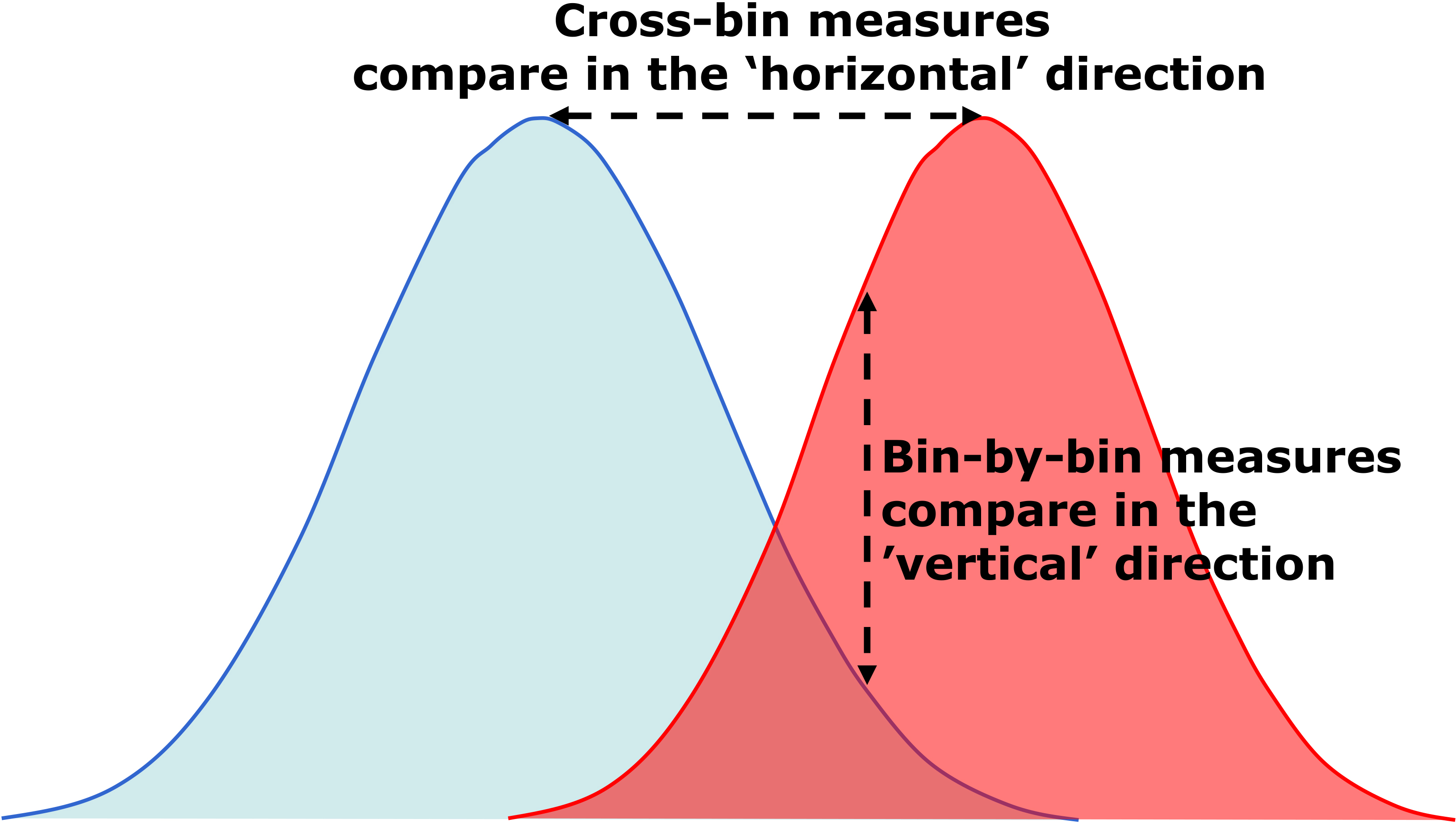

4. Bin-by-bin vs. cross-bin measures

Borrowing the terminology introduced by [21] we divide all dissimilarity measures into two large groups: bin-by-bin measures and cross-bin measures. The fundamental difference between the two groups of measures can be intuitively grasped by the graphical representation in Fig. 4.6

⁶
Credit: Figure was inspired by the original image appearing in J. Kun’s blog available at: https://jeremykun.com/2018/03/05/ earthmover-distance (accessed December 20th, 2023).

Bin-by-bin measures tend to capture the “vertical” gap between map values in each bin, regardless of the bin location, while while cross-bin measures (and most prominently KWD) attempt to capture the “horizontal” displacement.

4.1 Bin-by-bin measures

In Table 1 we report a partial list of different measures found in the literature. All such measures are based on the same common structure:

$\displaystyle M\left(\bm{u},\bm{v}\right)=g\left(\sum_{i}{f\left(u_{i},v_{i}% \right)}\right)$ (1)

wherein some outer transformation function $g()$ is applied to the sum over the bins of some inner function $f\left(u_{i},v_{i}\right)$ . The inner function captures the dissimilarity between the map values in each individual bin independently from all other bins. Notably, neither the bin coordinates $(a_{i},b_{i})$ nor the inter-bin distances $d_{ij}$ enter into the equation. In other words, the structure of Eq. (1) is completely oblivious to the spatial arrangement of the bins, to their relative ordering and to their mutual proximity or nearness relations. Not even the fact that bins are arranged in a 2-dimensional pattern is taken into account. The measures in Table 1 could well be applied to distributions defined over bins representing categorical variables defined over an arbitrary $\ell$ -dimensional abstract space. We remark that, when dealing with spatial distributions defined over the geographical domain, it is at least curious, if not paradoxical, that the structural properties of the geographical domain do not play any role at all.

Recall that a measure $M\left(\bm{u},\bm{v}\right)$ must satisfy four axiomatic properties in order to constitute a true distance metric:

The distance from any point to itself is zero: $M(\bm{u},\bm{u})=0,\quad\forall\bm{u}.$

Positivity: $M(\bm{u},\bm{v})\geqslant 0,\quad\forall\bm{u}\neq\bm{v}.$

Symmetry: $M(\bm{u},\bm{v})=M(\bm{v},\bm{u}),\quad\forall\bm{u},\bm{v}.$

Triangular inequality: $M(\bm{u},\bm{v})\leqslant M(\bm{u},\bm{z})+M(\bm{z},\bm{v}),\quad\forall\bm{u}% ,\bm{v},\bm{z}.$

Notably, not all the measures given in Table 1 are distance metrics. Note also that some of the measures are defined only for bins with non-zero mass (typically due to the function $f()$ embedding a logarithm transformation).

As noted above, bin-by-bin measures fail to capture the geographical nature of the distribution domain, and therefore the spatial displacement error that may be at play in spatial applications. Recalling Section 3, let us consider the case where one argument, say $\bm{u}$ , represents the “true” distribution value and the other argument $\bm{v}$ an estimated/measured value thereof. The estimation/measurement method is such that a generic unit of mass placed in bin $i$ in the true map $\bm{u}$ may be accounted for in a different bin $j\neq i$ in the estimated/measured map $\bm{v}$ . In this case, the inter-bin distance $d_{ij}$ represents the magnitude of the spatial displacement error for the generic unit of mass under consideration. What we demand from a “good” estimation/measurement method is to minimise not only (i) the amount of displaced mass (equivalently, the amount of mass affected by non-zero displacement), but also (ii) the magnitude of the displacement $d_{ij}$ . Clearly, bin-by-bin measures fail to capture the latter aspect. To illustrate the consequence, let us consider the simple toy-case depicted in Fig. 2 where the true map $O$ has the entire mass located in a single bin (marked with a red dot in the figure) and the other three maps $A$ , $B$ and $C$ represent different estimates/measurements obtained with different methods. The three estimates are all affected by a loss of spatial resolution, with the estimated mass diluted uniformly over the nine tiles marked in grey. The dilution of precision is the only error effect in estimate $A$ , hence the grey area remains centred around the true mass location. For estimate $B$ instead, there is also an additional shift (bias) towards the bottom-left corner. Finally, the estimate $C$ yields a more scattered pattern, with the grey tiles spreading out to non-adjacent locations.

Figure 2.

Toy Example # 1. All bin-by-bin measures would yield 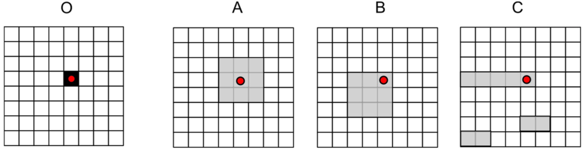$M(O,A)=M(O,B)=M(O,C)$ .

In this small simple example the goodness ordering is rather obvious: map $A$ is the most accurate estimate of $O$ , $B$ is the second best and $C$ is the worst one. However, none of the measures listed in Table 1 is able to differentiate between the three maps: it is trivial to verify that all such measures would deliver exactly the same dissimilarity value from the true map for all three options, i.e., $M(O,A)=M(O,B)=M(O,C)$ . In fact, the three maps differ in the location of the grey bins, hence in their neareness to the “true bin” (marked with a dot) but this aspect is completely missed by bin-by-bin measures. In other words, “vertical” bin-by-bin measures are completely oblivious to the location of the mass values, i.e., to the magnitude of the horizontal displacement. Other examples highlighting the limitation of bin-by-bin measures vis-à-vis cross-bin measures are presented e.g in [9].

4.2 Cross-bin measures

Having established the main imitation of bin-by-bin measures, we are interested to explore alternative measures that are able to capture the magnitude of the displacement error in addition to the amount of displaced mass. To do so, we must consider measures that are able to take into account the structural properties of the underlying geographical domain. Such class of measures was called “cross-bin measures” in [21]. Again inspired by Fig. 4 we shall refer to this group as “horizontal” measures to distinguish them from the “vertical” bin-by-bin measures introduced earlier.

KWD is a prominent example of cross-bin measure in the sense defined by [21]. Another example of cross-bin measure given in [21] is the quadratic form $M=\sqrt{(\bm{v}-\bm{u})^{T}\bm{A}(\bm{v}-\bm{u})}$ wherein the $n\times n$ matrix $\bm{A}$ represents the ground distance between all bin pairs. Very recently, a novel cross-bin measure for 2-dimensional histograms based on the 2D Fourier transform was studied in [4, 3]. In the present paper we focus exclusively on KWD as introduced formally in Section 5. Notably, all the three cross-bin measures mentioned in this paragraph are distance metrics.

4.3 Discussion

Having introduced the notions of “vertical” bin-by-bin and “horizontal” cross-bin measures, we now present some qualitative considerations concerning the relation between vertical measures and spatial displacement error.

We start from the consideration that any horizontal displacement (i.e., misplacing a unit of mass from tile $i$ to tile $j$ ) produces also some vertical deviation (i.e., an underestimation in tile $i$ and overestimation in tile $j$ ). In other words, there is a certain coupling between horizontal displacement and vertical deviation. Therefore, even bin-by-bin measures capture indirectly, at least to some extent, the horizontal displacement error.

If the coupling is sufficiently strong, then for practical purposes it may suffice to use some bin-by-bin measure to capture (indirectly) the horizontal displacement, with no need to resort to computationally heavier cross-bin measures. In other words, we may consider some simpler bin-by-bin measure as a good proxy for the more complex cross-bin measure. However, this “proxy” approach is viable only when the analyst knows or may safely assume in advance that a strong coupling is in place between horizontal displacement and vertical deviation for the particular application at hand. This is not always the case, and for instance it was not the case with the examples depicted in Fig. 2.

At this point it is natural to raise the question: How well is a bin-by-bin measure able to capture (partially, indirectly) the displacement error? Or equivalently: How well may a bin-by-bin measure serve as proxy for a cross-bin measure?

Speaking qualitatively, the answer depends on the particular conditions of the problem instance at hand, and specifically on the interplay between (a) the displacement mechanism and (b) the spatial distribution patterns. At one extreme, in some special cases the horizontal error induces a particular pattern of vertical deviation that is well captured also by a bin-by-bin measure, and therefore the latter is an excellent proxy for cross-bin measure. At the other extreme, we may have situations conceptually similar to the simple example shown in Fig. 2, where the horizontal displacement pattern cannot be “decoded back” from the vertical deviation effect that it produces, and bin-by-bin measures would be completely inadequate.

Conducting an exhaustive assessment goes beyond the scope of the present contribution and is left for future investigation. Here it suffices to say that in certain applications, where the displacement mechanisms and their vertical deviation effects are well understood, it may be sufficient to adopt a bin-by-bin measure as a lighter proxy for the more computationally expensive cross-bin approaches. However, such situations should be considered as special cases, not representative of general situations. In exploratory research, and in general when the mechanisms at play are not (yet) well understood, resorting exclusively to bin-by-bin measures carries a high risk of incurring experimental fallacies. It would be better in such conditions to consider a set of multiple dissimilarity measures that include also some cross-bin measures, with KWD being a natural candidate to be considered for the latter group.

5. The Kantorovich-Wasserstein Distance

5.1 Overview

The Kantorovich-Wasserstein Distance (KWD) is known with several alternative names, see [5, 10] and references therein. It corresponds to the Wasserstein-1 distance, a special case of the Wasserstein- $p$ (Wasserstein distance of order $p$ ) for $p=1$ . In Computer Science it is often known as Earth Mover Distance. KWD can be defined for continuous distributions as well as for discrete contributions. In this work we consider exclusively the discrete form that is relevant for binned distributions.

KWD was originally introduced in the field of Optimal Transport [17, 22] and later adopted in the field of Image Processing [21], Machine Learning [1] and Statistical Inference [6], often with the name of “Wasserstein distance” or “Earth Mover Distance”.

The application of KWD as a tool for data analysis has recently started to spread across Earth sciences, from Meteorology [9] and Geology [14] to Hydrology [15] and Oceanography [12]. While obviously the physical quantity of interest varies across the different scientific domains (from chemical pollutants density to rainfall intensity, from grain size to chlorophyll concentration, to stay with the cited papers), we can identify a few prominent use-cases for KWD as a descriptive tool that are transversal to the different domains. First, KWD is used to perform model-to-data comparison, i.e. to quantify the (dis)agreement between spatial distributions obtained from model-based predictions or simulations and real-world data obtained from in situ measurements. Second, KWD is used to quantify temporal changes, i.e., to condense into a scalar value the variation across time of the spatial distribution of the quantity of interest. Third, KWD can be leveraged to summarise multiple distributions through the concept of “Wasserstein barycenter”: given a set of $K\leqslant 2$ input maps (corresponding e.g. to real-world measurements at different times or predictions by different models of the same quantity of interest), the Wasserstein barycenter represents the map (not necessarily included in the input set) that yields the minimum KWD from the $k$ input maps, and therefore can be taken as a representative summary of the whole set of $K$ inputs in alternative to the classical bin-by-bin averaging (see e.g. [15, 2] and references therein).

On the practical side, one key issue to be considered when using KWD is the relatively high computational complexity that prevents the computation of the exact value for very large maps. However, the recent work by Bassetti, Gualandi and Veneroni [5] has shown that a close approximation, within a provable deterministic bound, can be computed in reasonable time on standard off-the-shelf machines, paving the way towards the application of KWD also to large maps of practical interest for spatial statistics. The approach proposed by Bassetti, Gualandi and Veneroni [5], hereafter referred as the “BGV method” for short, is the basis for the open-source tool Spatial-KWD . In the rest of this section we first introduce the exact KWD definition and then present the BGV method.

5.2 Exact definition

Let us start considering the basic case where the two maps have equal total mass, i.e. $\|\bm{u}\|_{1}=\|\bm{v}\|_{1}=m$ (the case of unequal masses will be addressed later in Section 6.2). In a nutshell, KWD between $\bm{u}$ and $\bm{v}$ can be interpreted as the minimum cost of transporting the mass (or “moving the earth”) from configuration $\bm{u}$ into $\bm{v}$ , or vice-versa, when the cost of moving a unit of mass is proportional to the Euclidean distance between the source and destination bins.

In order to formalise the concept of minimum cost, it is convenient to represent the grid as a directed graph $\mathcal{G}^{\prime}\lx@stackrel{{\scriptstyle\textrm{\@setsize{\tiny}{6pt}{% \vpt}{\@vpt}def}}}{{=}}\{\mathcal{B},\mathcal{L}^{*}\}$ where the set of nodes $\mathcal{B}$ corresponds to the set of $n$ bins, and the set of directed links $\mathcal{L}^{*}$ correspond to all $n(n-1)$ ordered node pairs. An example of the complete graph for a toy grid of $n=9$ bins is represented in Fig. 3(a).

With these positions, and recalling that we have assumed equal total mass between the two arguments $\|\bm{u}\|_{1}=\|\bm{v}\|_{1}$ , KWD can be expressed as the solution of the following Linear Programming (LP) problem:

$\displaystyle\begin{array}[]{lll}\text{minimise}&C(\bm{u},\bm{v})\lx@stackrel{% {\scriptstyle\textrm{\@setsize{\tiny}{6pt}{\vpt}{\@vpt}def}}}{{=}}\frac{1}{m}% \displaystyle\sum\limits_{i}{\sum_{j}{x_{ij}d_{ij}}}\\ \text{subject to}&\displaystyle\sum\limits_{i}{x_{ji}}=u_{j}\quad\forall\,j\in% \mathcal{B}\\ &\displaystyle\sum\limits_{i}{x_{ij}}=v_{j}\quad\forall\,j\in\mathcal{B}\\ &x_{ij}\geqslant 0\quad\quad\quad\forall\,(ij)\in\mathcal{L}^{*}\end{array}$ (2)

wherein all sums run over the links included in $\mathcal{L}^{*}$ . This formulation with transport cost proportional to the Euclidean distance $d$ is a special case of the more general formulation of the Wasserstein distance of order $p$ (or Wasserstein- $p$ distance) where the cost is proportional to $d^{p}$ . In this paper we consider exclusively the case $p=1$ (Wasserstein- $1$ or equivalently KWD) for which the transport cost has a direct physical interpretation in terms of Euclidean distance.7

⁷

Replacing $d$ with $d^{p}$ in the LP problem (2) leads to the general form of the Wasserstein- $p$ distance, or equivalently, Wasserstein distance of order $p$ . It should be noted that the BGV approximation method presented later in the paper applies only to $p=1$ and does not generalise to $p>1$ .

In the LP problem (2) the $x_{ij}$ ’s act as variables while $d_{ij}$ ’s, $u_{i}$ ’s and $v_{j}$ ’s act as parameters. The solution to the minimisation problem will be denoted by $C(\bm{u},\bm{v})$ and represents the exact value of KWD between the argument maps $\bm{u}$ and $\bm{v}$ .

Figure 3.

Example of transportation graph for a regular grid of 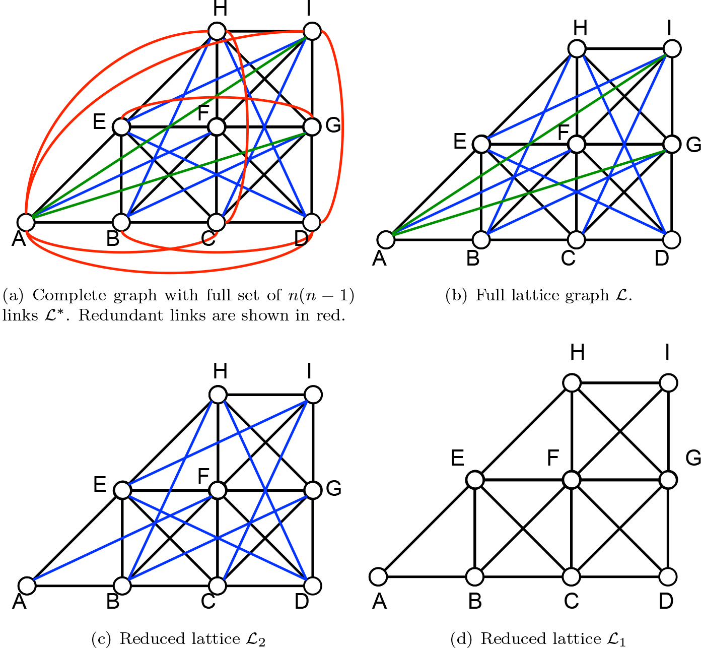$n=9$ nodes.

The very same solution to the LP problem (2) can be obtained by considering a reduced graph obtained from $\mathcal{L}^{*}$ by pruning all redundant links, along with a slight modification of the LP problem formulation. The notion of redundant link can be immediately grasped by comparing Figs 3(a) and 3(b): the direct link from node (bin) A to node C is redundant in the sense that an alternative path exists yielding exactly the same (minimum) cost, in this case through node B. Therefore, if the optimal transport solution involves the transportation of mass from node A to node C, in principle such mass may be moved either through the direct link $\overline{\text{AC}}$ or through the path $\overline{\text{ABC}}$ . In the latter case, node B serves purely as a transit node. The LP formulation (2) does not allow nodes to serve as transit nodes, and always requires the existence of a direct link from the source to the destination node. In order to enable transport routes passing through transit nodes, we must resort to a slightly different LP formulation, replacing the pair of mass conservation constraints in (2) with a single balancing constraint, leading to the new equivalent formulation (3) below. With the new formulation, the direct link $\overline{\text{AC}}$ becomes redundant and can be eliminated. Similar considerations apply e.g. to the direct link $\overline{\text{AH}}$ , which is redundant due to the presence of the same-length path $\overline{\text{AEH}}$ path, and so on. After pruning all redundant links, the new resulting set of links will be denoted by $\mathcal{L}\subseteq\mathcal{L}^{*}$ (refer to Fig. 3(b) for the small grid example). Considering the new reduced graph, the new LP formulation writes:

$\displaystyle\begin{array}[]{ll@{\quad}ll}\text{minimise}&C(\bm{u},\bm{v})% \lx@stackrel{{\scriptstyle\textrm{\@setsize{\tiny}{6pt}{\vpt}{\@vpt}def}}}{{=}% }\frac{1}{m}\displaystyle\sum\limits_{i}{\sum_{j}{x_{ij}d_{ij}}}\quad&&\\ \text{subject to}&\displaystyle\sum\limits_{i}{x_{ji}}-\displaystyle\sum% \limits_{i}{x_{ij}}=u_{j}-v_{j}\quad&\forall\,j\in\mathcal{B}\\ &x_{ij}\geqslant 0\quad&\forall\,(ij)\in\mathcal{L}\end{array}$ (3)

wherein all sums run over the links included in $\mathcal{L}$ . Again, we shall denote by $C(\bm{u},\bm{v})$ the solution to the minimisation problem that still represents the exact KWD value due to the equivalence between the LP problems (2) and (3).

Note the different structure of the constraint in the two formulations (2) and (3). In the latter, a single balancing constraint is imposed on the generic node $j$ forcing the net outbound flow $\sum_{i}{x_{ji}}-\sum_{i}{x_{ij}}$ , i.e., the difference between the total outbound flow $\sum_{i}{x_{ji}}$ and the total inbound flow $\sum_{i}{x_{ij}}$ , to equal exactly the difference between the initial ( $u_{j}$ ) and final ( $v_{j}$ ) mass values. This single constraint, that replaces the pair of separate constraints appearing in formulation (2) for the inbound and outbound flows, allows the generic node $j$ to serve as transit node for mass originated from and arriving to other nodes.

The optimal solution $C(\bm{u},\bm{v})$ of problem (3) on the reduced link set $\mathcal{L}$ equals the solution of problem (2) on the full link set $\mathcal{L}^{*}$ . However, eliminating the redundant links reduces the size of the problem, hence the computational cost.

Figure 4.

Bound (4) as a function of parameter 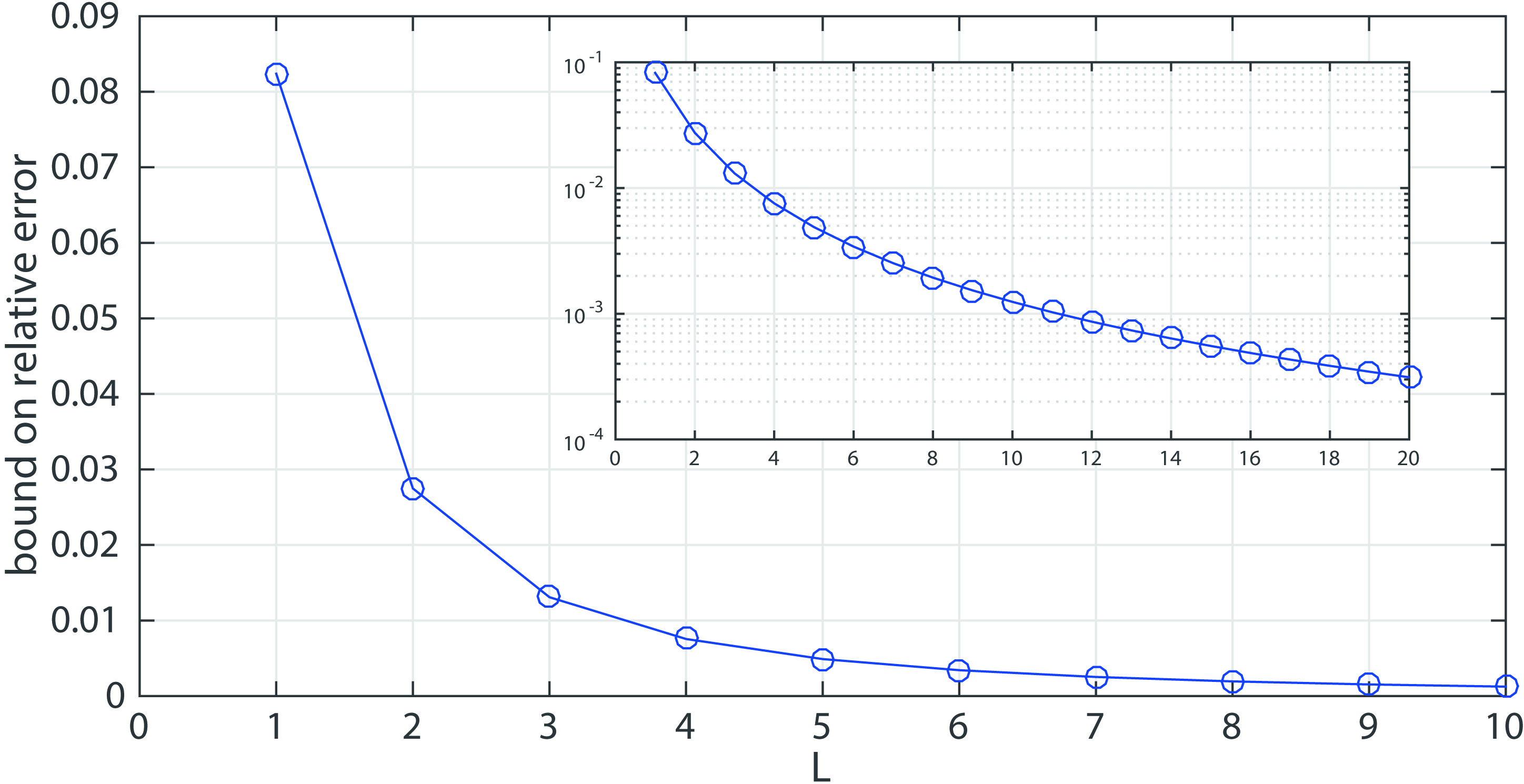$L$ .

5.3 Approximations on regular lattices

To further reduce the computational cost, we can run the LP problem (3) on a subset of the full lattice graph. However, the solution obtained in this way will be close, but not exactly equal to the KWD value computed on the full latice graph $C(\bm{u},\bm{v})$ . The BGV method developed in [5] considers a parametrised family of regular lattices (for regular square grids) where two generic nodes at coordinates $(a_{i},b_{i})$ and $(a_{j},b_{j})$ are connected only if $(a_{j}-a_{i})$ and $(b_{j}-b_{i})$ are coprime and $\max(a_{j}-a_{i},b_{j}-b_{i})\leqslant L$ , wherein $L\in\{1,2,\ldots\}$ is an integer parameter. To illustrate, we report in Fig. 3(c) and 3(d) the graphs, respectively, for $L=2$ and $L=1$ for the simple example at hand.

Denote by $\mathcal{L}_{L}$ the graph corresponding the parameter value $L$ and by $C_{L}(\bm{u},\bm{v})$ the solution of LP problem (3) over the reduced graph $\mathcal{L}_{L}$ . The following ordering relations hold:

$\mathcal{L}_{1}\subseteq\mathcal{L}_{2}\ldots\subseteq\mathcal{L}_{L}\subseteq% \mathcal{L}_{L+1}\ldots\subseteq\mathcal{L}\subseteq\mathcal{L}^{*}$

$C_{1}\geqslant C_{2}\ldots\geqslant C_{L}\geqslant C_{L+1}\ldots\geqslant C.$

In other words, increasing $L$ involves more and more links, hence higher and higher computation cost, but produces solutions that are closer and closer to the exact KWD value $C$ .

In their work Bassetti, Gualandi and Veneroni [5] make two key contributions. First, they show that, for a given value of $L$ , the solution $C_{L}(\bm{u},\bm{v})$ is itself a distance metric, i.e., it is non-negative, symmetric ( $C_{L}(\bm{u},\bm{v})=C_{L}(\bm{v},\bm{u})$ ) and satisfies the triangular inequality ( $C_{L}(\bm{u},\bm{v})\leqslant C_{L}(\bm{u},\bm{z})+C_{L}(\bm{z},\bm{v})$ ). Second, if $C_{L}(\bm{u},\bm{v})$ is regarded as an approximation of the KWD on the full graph $C(\bm{u},\bm{v})$ , they provide a deterministic bound to the relative approximation error $\varepsilon_{L}\lx@stackrel{{\scriptstyle\textrm{\@setsize{\tiny}{6pt}{\vpt}{% \@vpt}def}}}{{=}}\frac{C_{L}-C}{C_{L}}$ , formally:

$\displaystyle 0\leqslant\varepsilon_{L}\leqslant\Gamma_{L}\ \text{with}\ % \Gamma_{L}\lx@stackrel{{\scriptstyle\textrm{\@setsize{\tiny}{6pt}{\vpt}{\@vpt}% def}}}{{=}}1-\sqrt{\frac{1}{2}+\frac{L}{2\sqrt{1+L^{2}}}}.$ (4)

The value of the upper bound $\Gamma_{L}$ is plotted in Fig. 4 against $L$ and tabulated in Table 1. It can be seen that already with $L=$ 2 the worst-case maximum approximation error is below 3%, and $L=4$ is sufficient to bring the error below 1%. Furthermore, tests on benchmark data have confirmed that, as expected, the average approximation error is consistently lower than the worst-case error bound (4) by several orders of magnitude. Therefore, a small value of $L$ is sufficient in most practical applications (also considering that the discretisation of the geographical space in a regular grid is itself a form of approximation) enabling the computation of (closely approximated) KWD values for very large maps. The recommended default value in Spatial-KWD is set to $L=3$ , corresponding to a worst-case error below 1.3%.

5.4 Spatial-KWD implementation

The Spatial-KWD tool builds upon the BGV method from [5]. At its core, the tool builds the LP problem (3) and solves it through an advanced version of the simplex algorithm [7, 13]. The package is developed in standard C++11 and provides wrappers for R and Python. The R wrapper is based on RCPP [8]. The open-source code is publicly available under EUPL 1.2 license at the links that are given at the end of the paper.

To give an a idea of the run-time that may be expected by practitioners, we report in Table 2 the execution times obtained on a commercial workstation (DELL 7960, 56 cores, 4 GHz, 128 GB RAM, running Ubuntu Linux 22.04 LTS) for pairs of semi-synthetic benchmark maps covering the whole Belgium at different resolutions.8

⁸
The benchmark maps were derived from the real-world 2020 census grid at 1 $km^{2}$ resolution published by STATBEL https://statbel. fgov.be/en/open-data/population-according-km2-grid-2020. The distribution at finer resolutions was obtained by spreading randomly the value of each 1 $km^{2}$ cell across smaller inner cells. For each resolution level, the semi-synthetic map produced in this way was compared with a randomly perturbed version. The benchmark maps are publicly available from https://github.com/eurostat/Spatial-KWD/releases/download/v0.4.1-alpha/synthetic.tar.gz.

The run-time values were obtained for

L=3

, corresponding to a worst-case approximation error below 1.3% (but the average approximation error is several order of magnitude smaller and practically negligible already for

L=3

). The results show that, for maps covering the whole Belgium, Spatial-KWD delivers the final result in less than 2 seconds for 1 km

\times

1 km resolution, in less than half a minute for 500 m

\times

500 m resolution, in a few minutes for 250 m

\times

250 m resolution, and in about 2–3 hours for the finest resolution level of 125 m

\times

125 m corresponding to c.ca 2.5 millions bins.

Table 2

Run-time of Spatial-KWD on a commercial desktop for benchmark maps covering the whole Belgium at different grid resolutions ( $L=3$ )

Grid resolution [meters]	Num. nodes	Num. arcs	Mean – max time
$1000\times 1000$	39 392	64 624	1.5–1.7 sec
$500\times 500$	156 239	235 913	19.3–29.6 sec
$250\times 250$	621 868	936 527	7.2–13.9 min
$125\times 125$	2 482 109	3 768 938	2.4–4.9 hrs

6. Options for practical applications

The Spatial-KWD tool embeds additional features meant to facilitate its use across diverse application domains. In fact, KWD is an abstract mathematical concept and its adoption in practical analysis tasks involves a number of methodological design choices. Given a particular analysis task, the issue is not only whether KWD is a meaningful measure for the task at hand vis-à-vis other alternative measures, but rather how KWD can be applied meaningfully to the task. Practitioners should remain aware that even the “right” tool can be used in the “wrong” way. Furthermore, thw “right” way to apply KWD for one analysis task may be “wrong” for some other task.

In this section we describe some of the principal issues that practitioners will likely encounter when using KWD for practical tasks in spatial statistics. For each of them, we present the range of options that are currently supported by the Spatial-KWD tool. In fact, the tool was developed with a rich set of features and options in order to enable its use across a diverse range of application domains.

6.1 Non-convex regions

In practical applications, the region of interest may have an irregular shape, corresponding for instance to a whole country or to some administrative unit. If the region is convex, by definition all direct segments between any pair of bins (or more exactly, bin centers) lie entirely within the region. Instead, for a non-convex region this condition is not always satisfied. Figure 5 shows an example of non-convex region with two examples of bin pairs for which the direct path (red dashed line) crosses the region border. For such bin pairs, the question arises as to whether the link cost should be set equal to the unconstrained Euclidean distance (air distance, dashed red line) or, alternatively, to the shortest path constrained to lie entirely within the region of interest (geodetic distance, continuous green line). This is a design choice that depends on the application at hand, and specifically on the physical interpretation of the “displacement error” that we intend to capture by KWD. For example, if we are measuring the intensity of air pollutant that is not constrained to move within the region of interest, it is reasonable to consider the unconstrained distance. If instead we are considering density of people along a territory with a closed border that cannot be trespassed (e.g. a marine coast, or a barred border) we may opt for the constrained internal shortest path. This is a methodological design choice that depends on the application context, and the Spatial-KWD tool supports both options via a configurable parameter (refer to the documentation for details).

Figure 5.

Irregular non-convex region.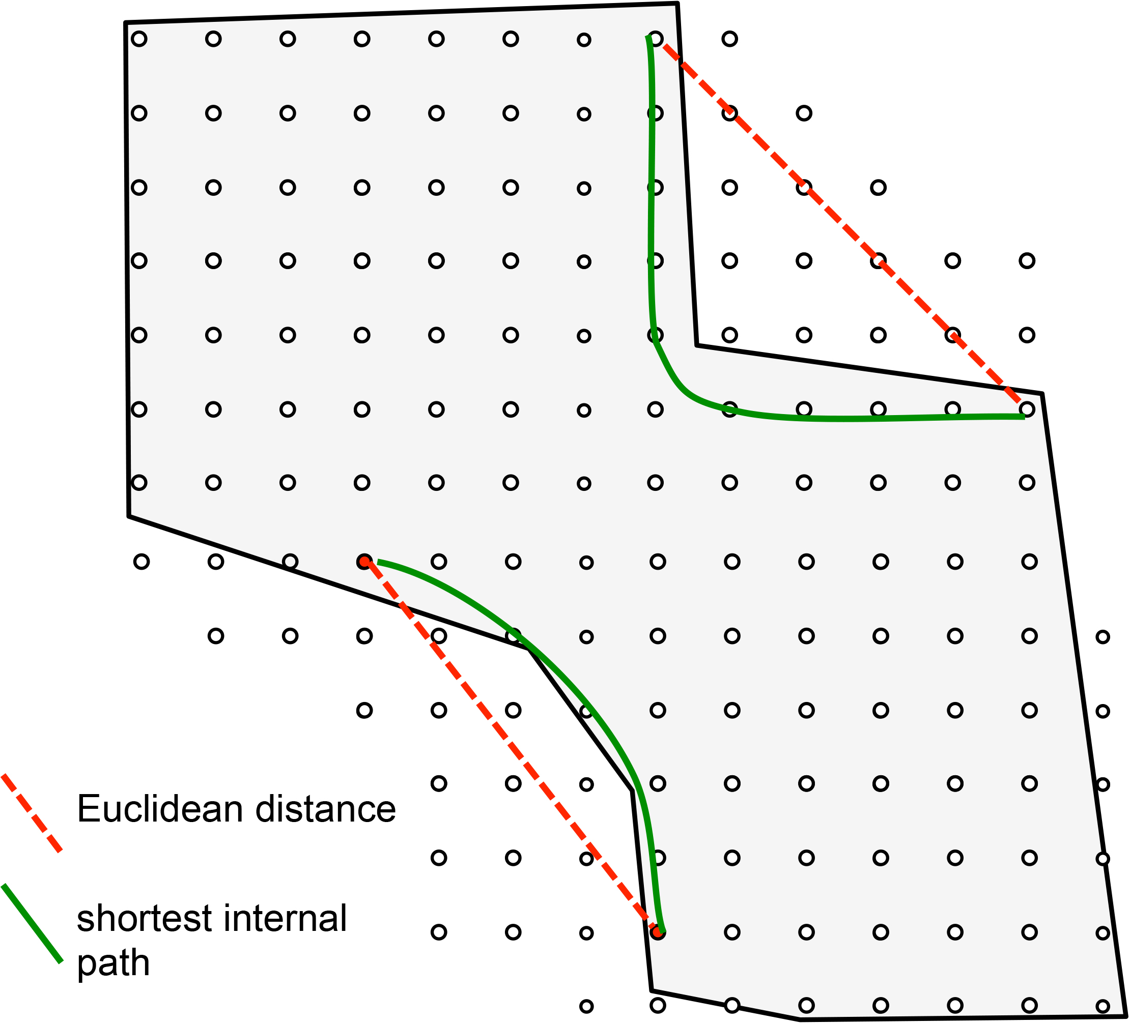

6.2 Unequal masses

Recall that the LP formulations given above require input arguments with same total mass, i.e., $\|\bm{u}\|_{1}=\|\bm{v}\|_{1}$ . In practical applications, maps with unequal masses may be encountered, e.g. when one input map represents the “ground truth” and the other some estimate thereof affected by total under- or over-estimation error on top of the spatial displacement error. In this section we discuss possible alternatives to cope with such a case.

Let $\Delta\lx@stackrel{{\scriptstyle\textrm{\@setsize{\tiny}{6pt}{\vpt}{\@vpt}def}% }}{{=}}\|{\mathbf{u}}-{\mathbf{v}}\|_{1}=\left|\sum_{i}u_{i}-\sum_{j}v_{j}\right|$ denote the total mass difference, or mass gap. From an algorithmic point of view, there are different ways to handle the extra mass, and the choice of one or other particular approach must be tied to the particular application at hand, and specifically to the physical interpretation of “mass” and to the (known or supposed) cause generating the mass gap. If the mass gap represents a global under-/over-estimation error, this entails considering the estimation error model.

In the following we review some of the possible options to deal with input maps with unequal masses. We start by distinguishing two general types of approach:

•
[Type-I] Methods that modify the original maps with unequal masses into a new pair of maps with equal masses on the same set of bins and links. The transformation is achieved by redistributing the mass gap $\Delta$ to the bins according to some criterion (e.g., multiplicative or additive).
•
[Type-II] Methods that augment the graph underlying the LP problem with one auxiliary “virtual bin”, to which the mass gap $\Delta$ is logically placed, and auxiliary “virtual links”. The two augmented maps then yield the same total masses equal to $m=\max{\left(\|\bm{u}\|_{1},\|\bm{v}\|_{1}\right)}$ . The virtual bin is connected to some or all physical bins via auxiliary “virtual links” of fixed cost $d_{\textit{aux}}$ . During the LP optimisation the mass gap is then “moved” between the virtual bin and the physical bins through the virtual links in a way that minimises the total transport cost. It can be demonstrated that, if the fixed cost $d_{\textit{aux}}$ is equal to or larger than the map diameter, i.e. $d_{\textit{aux}}\geqslant\max_{i,j}{d_{ij}}$ , then the solution to the augmented LP problem is still a distance metric [16].

Rescaling

In this Type-I approach, the maps are simply re-scaled or re-normalised. In other words, one computes $C(\bm{u^{\prime}},\bm{v}^{\prime})$ with $\bm{u}^{\prime}=\frac{\bm{u}}{\|\bm{u}\|_{1}}$ and $\bm{v}^{\prime}=\frac{\bm{v}}{\|\bm{v}\|_{1}}$ . This procedure is tantamount to implicitly spreading the mass gap $\Delta$ through all bins proportionally to the mass in each bin, therefore it is justified when the estimation error in each bin can be assumed to be roughly proportional to the mass in the same bin (multiplicative error). This simple approach is also justified when we are interested to assess the goodness of the relative distribution of mass in space, with no consideration for the total absolute value.

Flooring

Instead of adding the mass proportionally to the value in each bin, in this alternative Type-I approach the gap mass is added uniformly over all bins as an additive constant value. In other words, assuming that $\|\bm{u}\|_{1}>\|\bm{v}\|_{1}$ , we compute $C(\bm{u},\bm{v}^{\prime\prime})$ with $\bm{v}^{\prime\prime}\lx@stackrel{{\scriptstyle\textrm{\@setsize{\tiny}{6pt}{% \vpt}{\@vpt}def}}}{{=}}\bm{v}+\frac{\|\bm{u}\|_{1}-\|\bm{v}\|_{1}}{n}>\bm{v}$ . This simple approach is suited whenever the estimation error in each bin can be assumed roughly independent from the mass of each bin and distributed uniformly over the area of interest (additive error).

Virtual bin with fixed-cost virtual links

With the previous Type-I methods, the extra mass is positioned in the area of interest according to an explicitly criterion, i.e., proportionally to the bin value (rescaling) or as a constant term (flooring). In both cases, this approach requires making a “hard” design choice about the geographical distribution of the mass gap.

Type-II methods follow a completely different rationale: they assign the extra mass to an auxiliary “virtual bin”, connect the virtual bin with fixed-cost “virtual links” to a subset of the geographic bins (possibly all), and then let the optimisation process find the “best” way to reallocate the mass gap to the physical bins. This approach requires a slight modification of the LP problem, or more precisely of the support graph underlying the LP problem, to incorporate the auxiliary virtual bin and the corresponding virtual links. The links to and from the auxiliary bin are assigned a fixed cost $d_{\textit{aux}}$ whose value can be configured by the analyst. In practical applications we expect this cost to be set equal to or higher than the physical map diameter, formally $d_{\textit{aux}}\geqslant\max_{i,j}{d_{ij}}$ , based on the consideration that the penalty for missing a unit of mass should be higher than the penalty for displacing it in the wrong bin. The Spatial-KWD tool allows to set freely the value of parameter $d_{\textit{aux}}$ .

Figure 6.
Examples of Type II approaches to handle unequal masses. The auxiliary “virtual bin” gets assigned the mass gap and, from there, it can flow to a subset of physical bins (i.e., insertion points) through auxiliary “virtual links” of fixed cost 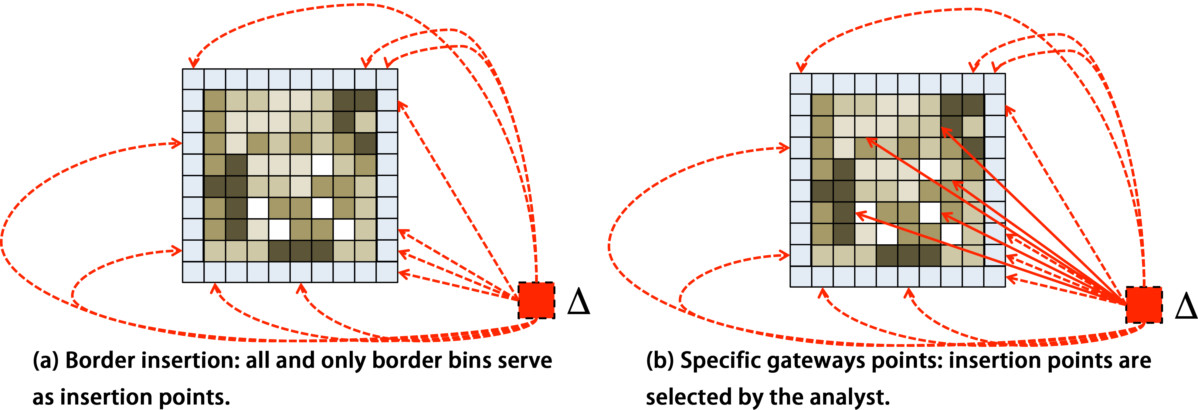$d_{\textit{aux}}$ .

Figure 7.
Two examples illustrating the FA concept. For each scenario (top and bottom row, respectively) the figure shows three distinct transport plans and corresponding KWD values: (a) globally optimised transport plan for the whole area of interest; (b) transport plan obtained with the naif approach of cropping the FA, ignoring all nodes and mass falling outside, and applying the standard optimisation to the cropped FA map; (c) local transport plan obtained with the FA formulation implemented in Spatial-KWD, taking into account external mass in the vicinity of (but not necessarily adjacent to) the FA.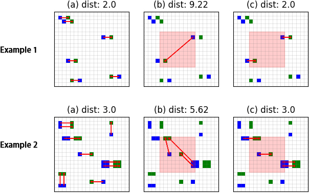

The physical bins connected to the auxiliary virtual bin represent the (physical) insertion points of extra mass. Configuring the set of insertion points represents a methodological design choice, but a softer one than the direct assignment of mass to bins as done in Type-I methods. The Spatial-KWD tool allows to configure freely which physical bins are connected to the virtual bin. Among the possible strategies for selecting the insertion points we highlight the following:

•
Ubiquitous insertion. All $n$ physical bins in the region of interest are configured to serve as insertion points.
•
Border insertion. Insertion points are limited to the border bins at the perimeter of the region of interest, as exemplified in Fig. 6(a).
•
Specific gateways. An arbitrary subset of bins are configured to serve as insertion points for the extra mass, as exemplified in Fig. 6(b). Such “getaway” bins may correspond to the location of qualified application-specific facilities (e.g., airports and train stations may serve as gateways for applications in the field of tourism and logistics, while factories may be relevant for applications in the field of environmental monitoring).

In summary, the Spatial-KWD tool provides great flexibility and customisation possibilities in handling the mass gap. For Type II methods, it supports the explicit configuration of the auxiliary link cost $d_{\textit{aux}}$ as well as the explicit selection of insertion points.
7. Local dissimilarity over a Focus Area

7.1 Motivations: global vs. local accuracy

The KWD between two maps is a summary indicator quantifying the dissimilarity between two input maps over the whole region of interest. When one input map represents the “true” distribution and the other some measured/estimated version thereof, KWD represents a summary indicator of the global accuracy of the measurement/estimation method at hand throughout the entire region of interest.

In some practical applications, we may be interested to assess the local accuracy in a specific sub-region of the larger region of interest. This is relevant, for instance, when the measurement/estimation process under evaluation is subject to large variations in the spatial accuracy due to local conditions.9

⁹
For example, the context of estimating present population based on Mobile Network Operator data [20], the local accuracy depends on the size of the deployed radio cells, that in turn depends on the local intensity of mobile traffic, with large differences between urban, sub-urban and rural areas. This is just one concrete example motivating the development of “local” dissimilarity measures in specific area (or sub-region) within a larger map.

More in general, understanding where the process yields higher vs. lower accuracy is instrumental to understand why it does so, i.e., under what spatial conditions it performs better or worse. In such a case, considering a single global figure for the whole area of interest would not provide sufficient insight, and it would be beneficial to develop a procedure for quantifying the local spatial error at a finer level of spatial detail, based on the computation of distance metrics with a local focus on a predefined sub-region. Towards this aim, we propose a novel variant of the KWD formulation that, in line with the spirit of KWD, aims at capturing the minimum transportation cost between two maps within a specified sub-region called “Focus Area” (FA) in Spatial-KWD .

Figure 8.

Focus area (FA) concept for localised metric. Continuous-line paths represent transportation flows entirely contained in FA. Dotted-line paths represent transportation flows between FA and the surrounding external bins.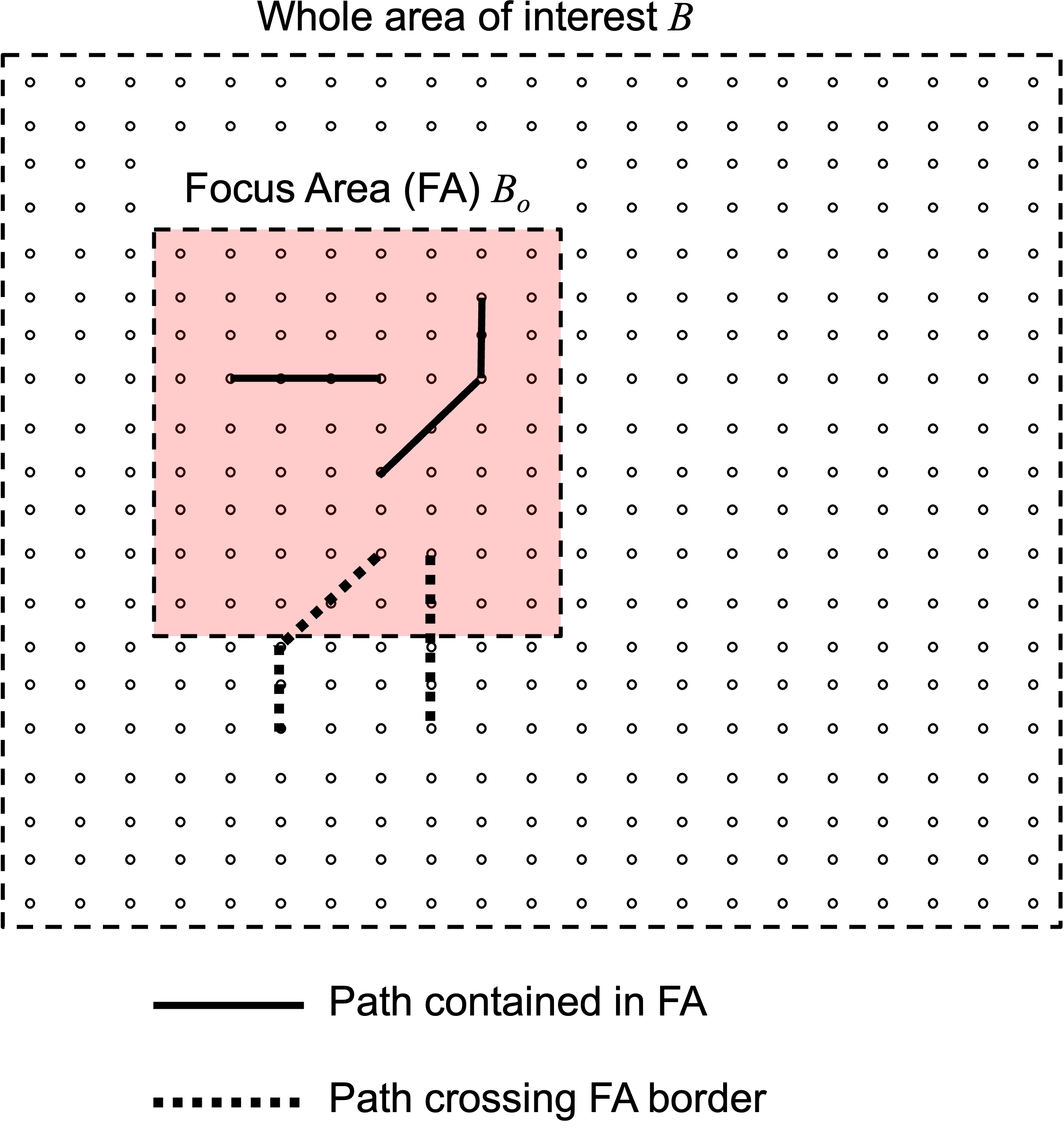

7.2 Fallacy of a naif approach

Before presenting our proposed approach, we explain the limitations of a naif approach. We do so by resorting to the two simple examples shown in Fig. 7. For each example, the figure reports three transport plans labelled (a), (b) and (c), with the corresponding minimum cost printed in each figure (labelled “dist.”). For each example the input maps, blue and green, are laid over the same $19\times 19$ area of interest in Fig. 7(a). Each coloured tile (equivalently: bin) hosts a single unit of mass while all the remaining uncoloured tiles are empty. Each of the two maps has a total mass equal to the number coloured tiles (blue or green) in each map. The optimal transport plan for the whole area of interest (red arrows in Fig. 7(a)) is rather homogeneous across the whole area of interest: each blue unit can be moved to the nearest green unit by an horizontal shift of exactly two tiles in the first example (top row), meaning that the global KWD between the two maps equals 2.0. Similarly, in the second example (bottom row) each blue unit can be moved to the nearest green unit by an horizontal or vertical shift of 3 tiles, resulting in a global KWD equal to 3.0. Now, assume we are interested to evaluate the local distance between the two maps within the 9 $\times$ 9 FA highlighted in red. Following a naif approach, we may just crop the two maps in the FA, ignore the map values (mass units) falling outside the FA, and solve the LP optimisation problem on a reduced grid corresponding solely to the FA. This operation would return the transport plan shown in 7(b) that is constrained “by design” to lie entirely within the FA. It is evident from the figure that this approach would introduce a major distortion in the optimal transportation plan, leading to a serious over-estimation of the transportation cost (9.22 instead of 2.0 in the first example, and 5.62 instead of 3.0 in the second one).

The problem with this approach is that all mass external to the FA, including the part thereof in the immediate vicinity of the FA, is completely ignored, thus forcing the transportation plan to rearrange exclusively the mass units internal to the FA. Furthermore, in practical applications it is likely that the cropping operation will return cropped maps with unequal masses, leaving to the analyst the decision to select one of the methods among those discussed in Section 6.2 to deal with unbalanced masses. Any choice would likely introduce additional distortion, since all the methods presented in Section 6.2 ignore the fact that the reduced map was sliced out of a larger map with a given mass distribution in the surroundings of the FA.

In order to mitigate such limitations, we propose hereafter a modified LP formulation that does not ignore the external mass outside the FA but treats it differently from the mass inside the FA. With the modified LP formulation given in Section 7.3, the transport plan computed for the FA would be the one shown in Fig. 7(c) for a minimum cost that is more in line with the global KWD value.

We remark that, in the general case, the local transport plan obtained in the FA with the proposed formulation is not guaranteed to correspond exactly to the globally optimised transport plan that would be obtained with a global minimisation across the whole area of interest without FA, and the local KWD value is not guaranteed to correspond exactly to the global KWD value. However, compared with the naif approach, the proposed formulation mitigates the kind of distortion illustrated above, leading to a transport cost value that is better representative of the local mass distribution.

7.3 Modified LP problem with FA

Let $\mathcal{B}_{\circ}\subseteq\mathcal{B}$ denote the pre-defined FA within the larger area of interest $\mathcal{B}$ , as sketched in Fig. 8. We wish to identify a procedure, based on the principle of minimum cost transport, to measure the local dissimilarity in $\mathcal{B}_{\circ}$ of two maps defined over the larger region $\mathcal{B}$ . To this aim, we consider a slightly modified LP formulation of the transport problem, with different balancing constraints imposed on the internal nodes (inside the FA) vis-à-vis the external ones (outside the FA).

For the generic node $j\in\mathcal{B}_{\circ}$ internal to FA we impose the same (balancing) equality constraint as in LP problem (3). Conversely, for the generic node $j\in\mathcal{B}\backslash\mathcal{B}_{\circ}$ external to FA we impose a pair of inequality constraints that cap separately the net outbound and inbound flows, respectively, to the initial and final mass value. In this way, we allow mass flow within the FA as well as between the FA and the outer surrounding area, but we impose the initial and final mass configuration to equal the input maps $\bm{u}$ and $\bm{v}$ only within the FA. The role of external nodes is only to provide to or absorb mass from FA as needed to fulfill the equality constraints therein.

The resulting LP formulation writes:

$\displaystyle\begin{array}[]{ll@{\quad}ll}\text{minimise}&C_{L}(\bm{u},\bm{v},% \mathcal{B}_{\circ})\lx@stackrel{{\scriptstyle\textrm{\@setsize{\tiny}{6pt}{% \vpt}{\@vpt}def}}}{{=}}\frac{1}{m_{\circ}}\displaystyle\sum\limits_{i}{\sum_{j% }{x_{ij}d_{ij}}}\quad&&\\ \text{subject to}&\displaystyle\sum\limits_{i}{x_{ji}}-\displaystyle\sum% \limits_{i}{x_{ij}}\!=\!u_{j}-v_{j}\quad\forall\,j\in\mathcal{B}_{\circ}\quad% \\ &\displaystyle\sum\limits_{i}{x_{ji}}-\displaystyle\sum\limits_{i}{x_{ij}}% \leqslant u_{j}\quad\forall j\in\mathcal{B}\backslash\mathcal{B}_{\circ}\quad% \\ &\displaystyle\sum\limits_{i}{x_{ij}}-\displaystyle\sum\limits_{i}{x_{ji}}% \leqslant v_{j}\quad\forall j\in\mathcal{B}\backslash\mathcal{B}_{\circ}\quad% \\ \par &x_{ij}\geqslant 0\quad\quad\quad\quad\quad\quad\quad\forall\,(ij)\in% \mathcal{L}_{L}\quad\end{array}$ (5)

wherein $m_{\circ}$ denotes the total mass that is actually moved.

The Spatial-KWD tool implements a modified problem that is equivalent to the LP formulation (5) and allows for more efficient resolution. In order to take advantage of efficient solvers for transportation flow problems with equality constraints, the LP problem (5) is transformed into an equivalent instance defined on a modified grid, where auxiliary nodes are inserted and connected with capacitated zero-cost auxiliary links to the nodes outside the external areas. With this trick, the inequality constraints in (5) are replaced by equality constraints, allowing the application of efficient solvers.

In the current version of the tool, the FA location and size can be specified as input argument, either in the shape of a square or near-circular area, by providing the coordinates of the FA center and FA radius as parameters: all tiles that are at L1 norm (for square) or L2 norm (for near-circular) distance from the center are included in the FA.

8. Conclusions and outlook on future work

In this paper we have presented the Spatial-KWD tool and illustrated its configuration features and options. We hope with this work to promote the consideration (and possibly the adoption) of the Kantorovich-Wasserstein Distance as a candidate dissimilarity metric in a wider range of spatial statistics applications. Spatial-KWD can be used to perform model-to-data comparison or to quantify the temporal changes in the spatial distribution of physical or social quantities, similarly to what is being pioneered in several Earth Science fields, from Meteorology [9] and Geology [14] to Hydrology [15] and Oceanography [12]. Our ready-to-use tool can support similar use-cases in other fields, from Environmental Statistics (distribution of pollutants) to Demography (distribution of present population).

At the time of writing, the tool has been used to support ongoing research on spatial density estimation of present population from Mobile Network Operator data [19, 18]. It was also considered for exploratory work in the field of Statistical Disclosure Control for spatial population grids [11]. We invite the statistical community to use the tool and share their experience with the authors, particularly for what concerns usability, new required features and indications for further development. The tools may be extended and enriched with additional features, and in this sense feedback from users and practitioners will help us to identify the most important direction for future development.

Among the possible venues for continuing this work, we would like to highlight the possible application of “Wasserstein barycenters” as a summarisation tool for (sets of) spatial distributions. As discussed earlier, when a set of $k\geqslant 2$ input spatial maps are given (e.g., the spatial distribution of present population in different working days) we may need to produce a single map that summarises “in the best way” the $k$ input maps (e.g., the “typical” population distribution in a working day). Intuitively, the optimal summary map is the one that minimises the distance from all $k$ input maps, but this general definition needs to be instantiated with a proper choice of the distance metric to be minimised. The simple approach of averaging the map value in each bin amounts to adopt implicitly some bin-by-bin metric, but in principle one may choose to minimise the KWD and in this way obtain the so-called “Wasserstein barycenter”. This approach has been recently explored in the fields of Pattern Recognition [2] and Hydrology [15] but is probably worth to be investigated also in other spatial statistics fields.

Disclaimer

The views expressed in this paper are those of the authors and do not necessarily represent the view of the European Commission.

Code

The open-source code of Spatial-KWD is publicly availabe under EUPL 1.2 license from https://github.com /eurostat/Spatial-KWD. The corresponding R package is available from the CRAN repository https://cran.r-project.org/web/packages/SpatialKWD and the corresponding Python implementation is available from pypi repository https://pypi.org/project/Spatial-KWD.

Footnotes

Acknowledgments

The implementation of Spatial-KWD was supported by Eurostat under Service Contract ESTAT.2020. 0257. The authors are grateful to Federico Bassetti from University of Milano for providing useful comments on an early draft of this work.

References

Arjovsky

Chintala

Bottou

. Wasserstein generative adversarial networks. In D. Precup and Y. W. Teh, editors, Proceedings of the 34th; International Conference on Machine Learning, volume 70 of Proceedings of Machine Learning Research, pp. 214-223. PMLR, 06–11 Aug 2017.

Auricchio

Bassetti

Gualandi

Veneroni

. Computing wasserstein barycenters via linear programming. In Integration of Constraint Programming, Artificial Intelligence, and Operations Research, pp. 355-363. Springer International Publishing, 2019. https//link.springer.com/chapter/10.1007/978-3-030-19212-9_23.

Auricchio

Codegoni

Gualandi

Toscani

Veneroni

. The equivalence of Fourier-based and Wasserstein metrics on imaging problems. Rendiconti Lincei. 2020; 31(3).

Auricchio

Codegoni

Gualandi

Zambon

Veneroni

. The Fourier discrepancy function. Communications in Mathematical Sciences. 2023; 21(3). doi: 10.4310/CMS.2023.v21.n3.a2.

Bassetti

Gualandi

Veneroni

. On the computation of Kantorovich-Wasserstein distances between two-dimensional histograms by uncapacitated minimum cost flows. SIAM Journal on Optimization. 2020; 3(6). doi: 10.1137/19M12611..

Bernton

Jacob

Gerber

Robert

. On parameter estimation with the Wasserstein distance. Information and Inference: A Journal of the IMA. 2019; 8(4): 657-676.

Cunningham

. A network simplex method. Mathematical Programming. 1976; 11.

Eddelbuettel

Francois

. Rcpp: Seamless R and C++ integration. Journal of Statistical Software. 2011; 40(8): 1-18.

Farchi

Bocquet

Roustan

Mathieu

Quérel

. Using the wasserstein distance to compare fields of pollutants: application to the radionuclide atmospheric dispersion of the fukushima-daiichi accident. Tellus B: Chemical and Physical Meteorology. 2016; 68(1): 31682.

10.

Gottschlich

Schuhmacher

. The shortlist method for fast computation of the earth mover’s distance and finding optimal solutions to transportation problems. Plos One. 2014.

11.

Gussenbauer

Jamme

de Jonge

de Wolf

P-P

Möhler

. Spatial SDC experiments and evaluations with multiple countries comparison. In UNECE Expert meeting on Statistical Data Confidentiality, Wiesbaden, Germany, September 2023; https//unece.org/sites/default/files/2023-08/SDC2023_S3_4_Austria_Gussenbauer_D.pdf.

12.

Hyun

Mishra

Follett

Jonsson

Kulk

Forget

Racault

M-F

Jackson

Dutkiewicz

Müler

Bien

. Ocean mover’s distance: using optimal transport for analysing oceanographic data. Proc. Royal Society A. 2022; 478(20210875).

13.

Kovács

. Minimum-cost flow algorithms: a n experimental evaluation. Optimization Methods and Software. 2015; 30(1).

14.

Lipp

Vermeesch

. Short communication: The wasserstein distance as a dissimilarity metric for comparing detrital age spectra and other geological distributions. Geochronology. 2023; 5(1): 263-270.

15.

Magyar

Sambridge

. Hydrological objective functions and ensemble averaging with the wasserstein distance. Hydrology and Earth Systems Science. 2023; 27: 991-1010.

16.

Pele

Werman

. Fast and robust earth mover’s distances. In 2009 IEEE 12th International Conference on Computer Vision, 2009; pp. 460-467.

17.

Peyré

Cuturi

. Computational optimal transport: with applications to data science. Foundations and Trends® in Machine Learning. 2019; 11(5-6): 355-607.

18.

Ricciato

Coluccia

. On the estimation of spatial density from mobile network operator data. IEEE Transactions on Mobile Computing. 2023; 22(6): 3541-3557.

19.

Ricciato

Lanzieri

Wirthmann

Seynaeve

. Towards a methodological framework for estimating present population density from mobile network operator data. Pervasive and Mobile Computing. 2020; 68.

20.

Ricciato

Widhalm

Craglia

Pantisano

. Estimating population density distribution from network-based mobile phone data. JRC Technical Report, 2015. Online: http//publications.jrc.ec.europa.eu/repository/bitstream/JRC96568/lb-na-27361-en-n.pdf.

21.

Rubner

Tomasi

Guibas

. The earth mover’s distance as a metric for image retrieval. International Journal of Computer Vision. 2000; 40. doi: 10.1023/A1026543900054.

22.

Santambrogio

. Optimal Transport for Applied Mathematicians: Calculus of Variations, PDEs, and Modeling. Birkäuser Cham, 2015.

The Kantorovich-Wasserstein distance for spatial statistics: The Spatial-KWD library

Abstract

Keywords

1. Introduction

1 Population and housing census 2021 available from https://ec. europa.eu/eurostat/statistics-explained/index.php?title=Population_ and_housing_census_2021_-_population_grids.

2 With this choice we aim at preserving continuity with previous literature from different research communities that had adopted one or the other term.

6 Credit: Figure was inspired by the original image appearing in J. Kun’s blog available at: https://jeremykun.com/2018/03/05/ earthmover-distance (accessed December 20th, 2023).

4.3 Discussion

5. The Kantorovich-Wasserstein Distance

5.1 Overview

5.2 Exact definition

6.1 Non-convex regions

Rescaling

Flooring

Virtual bin with fixed-cost virtual links

7.1 Motivations: global vs. local accuracy

7.3 Modified LP problem with FA

Disclaimer

Code

Footnotes

Acknowledgments

References

¹
Population and housing census 2021 available from https://ec. europa.eu/eurostat/statistics-explained/index.php?title=Population_ and_housing_census_2021_-_population_grids.

²
With this choice we aim at preserving continuity with previous literature from different research communities that had adopted one or the other term.

⁶
Credit: Figure was inspired by the original image appearing in J. Kun’s blog available at: https://jeremykun.com/2018/03/05/ earthmover-distance (accessed December 20th, 2023).