Assessing the multivariate distributional accuracy of common imputation methods

Abstract

Imputation methods are popular tools that allow for a wide range of subsequent analyses on complete data sets. However, in order for these analyses to be trustworthy, it is important that the imputation procedure reflects the true distribution of the unobserved data sufficiently well. This raises the question how well different imputation methods can reproduce multivariate correlations, associations or even the entire multivariate distribution. The paper gives first answers to this question by means of an extensive comparative simulation study. In particular, we evaluate the multivariate distributional accuracy for six state-of-the art imputation algorithms with respect to different measures and give practical recommendations.

1. Introduction

Missing data is a problem in many quantitative sciences. The reasons for missing information are manifold. Data can be lost after the survey or become unreadable due to technical problems. Or the respondents – for various reasons, deliberately or unconsciously – did not answer a question, so that no value can be stored for the corresponding feature. Another reason may be that a feature is not collected at all from some respondents, for example, to reduce the survey load. All these are cases of so-called item non-response. However, if complete data sets are expected despite item non-response (per se or because completeness is required for algorithmic processing), the missing data must be estimated. This is called imputation.

Immediately, however, the question arises when an imputation is “good”, how different imputation approaches can be compared and with respect to what measure an imputation should be optimized. To this end, there exist several different approaches [1], which was also studied in a recent work by Shadbahr et al. [2]. In our previous research [3], we focused on three different types of imputation accuracy: The predictive accuracy, the estimation accuracy after imputation and the distributional accuracy.

Predictive accuracy aims at estimating the missing values as accurately as possible, i.e. keeping the suitably measured distance between estimated and presumed true value as small as possible. Estimation accuracy, on the other hand, is less interested in the accurate estimation of missing values than in the accurate estimation of population parameters to be estimated from the available data set, for example, location measures, dispersion measures or correlation measures. If we know which population parameters are to be estimated and if their number is manageable at the time of imputation, we can often optimize the imputation for them. This is, e.g., common practice in the life and social sciences [4, 5, 6].

However, if there are too many population parameters to be estimated or if it is not even known at the time of imputation which evaluations are to be conducted later on the basis of the data set to be imputed, this optimization is not possible. This occurs, for example, when a data set is collected by one institution (e.g., a statistical office), completed by imputation, and then made available to another institution, the scientific community, or the public. In this case, the goal of imputation should be that the completed dataset has the same distribution (and thus, e.g., the same moments and quantiles) as the presumed true, complete dataset, i.e. distributional accuracy is of importance.

In our previous work [3, 7] we have already examined the univariate distributions of completed and presumed true data sets. This may be sufficient for location and dispersion measures of individual features, but for the analysis of dependencies between features (e.g., correlations) such a univariate approach is not sufficient.

It is the aim of the present paper to close this gap and evaluate distributional accuracy in a multivariate sense. Therefore it is of interest whether imputation reproduces the multivariate distribution of the entire data set appropriately. To this end, we consider measures that assess the multivariate distributional accuracy.

The paper is organized as follows. In Section 2 we describe the data underlying the simulation study, the missing settings and the employed imputation methods. We describe the measures to estimate the distributional accuracy in Section 3. Section 4 contains the details on the simulation study and its results. The paper concludes with a discussion of the results in Section 5.

2. Data set, missing settings and imputation methods

2.1 Data set and missing settings

2.1.1 Data set

For our simulation study, we use so-called Destatis campus files. Here, we use the data from the Structure of Earnings Survey from 2010, consisting of 25,974 anonymized observations on 33 variables. Since some of the variables contain missing values, we slightly modify the data set to run the simulation on a complete data set. A detailed description of the modifications can be found in [3, 8]. In addition, we removed variables from the data set that are irrelevant for the imputation, e.g., the identification numbers of the respondents. After these pre-processing steps, the data set contains 16 metric variables and 12 categorical variables. blackIt is not the aim of this paper to find an imputation method specifically suited for the Structure of Earnings Survey and explicitly to be used there. Rather, the Structure of Earnings Survey serves as a real example data set from official statistics for our investigations.

2.1.2 Missing settings

In our simulation study, we focus on two missing mechanisms: The Missing Completely at Random (MCAR) and the Missing at Random (MAR) mechanism [9]. In case of MCAR, the missings are independent from other (observed and unobserved) values of the data set. blackTo generate missing values under the MCAR mechanism, the R-function prodna from the missForest-package [10] is used. Therein, missing values are generated by randomly removing $\lceil r\cdot 100\rceil \in \mathbb{N}$ entries from the data set, where $r\in [0,1]$ is the missing rate. If the missing of the values depends on the observed values of the data set, but is independent from the theoretically observable missing values, MAR is present. blackIn the described simulation, missing data under the MAR mechanism is simulated according to a predefined logic, in which the values of one variable have an impact on the missingness in another variable:

1.

With an increasing age, the probability of a missing value for the (normalized) gross annual earning is decreasing.

2.

With a decreasing (standardized) weekly working time (ef53), the missing of the bonus for special working hours (ef23) increases.

3.

A missing value in the performance group (for employees with payment according to individual agreement; variable ef9) has the highest probability for employees with a “lower secondary education” (according to the ISCED scale; variable ef43). The second highest probability for a missing value is present for employees in the category “upper secondary education” and the lowest missing probability is present for people with a “tertiary education”.

2.2 Imputation methods

There exists a wide range of imputation methods [11] and it is almost impossible to compare the distributional accuracy of all of them. We therefore decided to compare only a few imputation methods which fulfill the following properties: they are (i) easy to use, (ii) implemented in the statistical software R [12], (iii) recommended from previous work and (iv) wide spread in statistical practice. This led us to five different imputation methods: black For single imputation, which means generating one complete data set for the incomplete data, the naive imputation method, which is for example described by van Buuren [11, p. 12], and the tree-based method missRanger [13] are used. In the naive method, the missing values of a variable are imputed by using the arithmetic mean (or mode for categorical variables) of the observed values. The broad idea of the tree-based imputation missRanger is to train a random forest on the the observed data which then use to predict (i.e. impute) the missing values. This idea was previously proposed by [10]. The implementation of missRanger is very similar to the implementation of missForest but the faster implementation ranger [14] is used. Additionally the R-package missRanger provides the option of using additional predictive mean matching for imputation. However, in order to be able to compare the results to other imputation methods, this option is not used for this simulation.

Besides these single imputation approaches, we used two algorithms for multiple imputation: Amelia and MICE. The difference to the single imputation methods is that for each incomplete data set, multiple (in our simulation five) complete data sets are generated. In the R-package Amelia [15], the missing data is imputed by applying the so-called EMB-algorithm, in which expectation-maximization is combined with bootstrapping. An often used imputation method is multiple imputation by chained equations (MICE) [16]. In the R-packages mice [17], multiple options for the concrete imputation are already implemented. For our simulation, we decided to focus on three mice options: imputation based on a Random Forest (Mice.RF), based on predictive mean matching (MICE.Pmm) and based on a normal (Bayesian) model (Mice.Norm). As the MICE.Pmm and Mice.Norm models do not allow imputation of categorical variables, all options impute ordinal variables by using the Random Forest based imputation. Further information on the aspects of the methods and the used implementation can be found in [3, 8].

3. Evaluation methods

In the following, we consider measures which can be used to assess the imputation methods’ multivariate distributional accuracy. We therefore focus on two aspects: dependencies between the variables (as measured by correlations) and the multivariate distributions themselves. For the latter, we consider the empirical distributions of linear combinations of the variables as well as the multivariate distributions estimated by Copulas. Due to a lack of convincing and simple multivariate approaches for categorical or mixed-type data we focus on the $d=$ 16 metric variables.

3.1 Correlation coefficients

An important aspect of a multivariate distribution are the dependencies among the variables of the data set. They can be estimated by different correlation coefficients. To assess imputation accuracy, we calculate the (empirical) correlation matrices of the imputed data sets ( $P^{\text{𝑖𝑚𝑝}}$ ) and compare them to the correlation matrix of the original data ( $P^{\text{𝑡𝑟𝑢𝑒}}$ ). We use Kendall’s $\tau$ , Pearson’s $r$ and Spearman’s $\rho$ to estimate linear as well as nonlinear relationships between the $d=16$ metric variables. To compare the correlation matrices of the imputed and original data, we take the differences between the correlation matrices of the imputed ( $P^{\text{𝑖𝑚𝑝}}$ ) and original ( $P^{\text{𝑡𝑟𝑢𝑒}}$ ) data set and calculate two different matrix norms: The Frobenius norm defined as:

${\parallel P^{\text{𝑡𝑟𝑢𝑒}}-P^{\text{𝑖𝑚𝑝}}\parallel }_F={\parallel {\left({\rho }_{ij}^{\text{𝑡𝑟𝑢𝑒}}-{\rho }_{\text{𝑖𝑗}}^{\text{𝑖𝑚𝑝}}\right)}_{i,j\in 𝒩}\parallel }_F={\left({\displaystyle \sum _{i\in 𝒩}}{\displaystyle \sum _{j\in 𝒩}}{\left({\rho }_{ij}^{\text{𝑡𝑟𝑢𝑒}}-{\rho }_{\text{𝑖𝑗}}^{\text{𝑖𝑚𝑝}}\right)}^2\right)}^{\frac{1}{2}},$

where $𝒩=\{1,\mathrm{\dots },16\}$ corresponds to the $16$ metric variables. Moreover, we compute the Maximum norm given by:

${\parallel P^{\text{𝑡𝑟𝑢𝑒}}-P^{\text{𝑖𝑚𝑝}}\parallel }_M={\parallel {\left({\rho }_{ij}^{\text{𝑡𝑟𝑢𝑒}}-{\rho }_{\text{𝑖𝑗}}^{\text{𝑖𝑚𝑝}}\right)}_{i,j\in 𝒩}\parallel }_M=\underset{\begin{array}{c}i,j\in 𝒩\end{array}}{\max }\left|{\rho }_{ij}^{\text{𝑡𝑟𝑢𝑒}}-{\rho }_{\text{𝑖𝑗}}^{\text{𝑖𝑚𝑝}}\right|.$

This leads to a single value for each imputed data set. For the multiple imputation methods, we averaged the $m=5$ observed values of the norms.

3.2 Kolmogorov-Smirnov-Statistics for linear combinations

As in our previous work [3, 8], we study distributional distance measures to measure imputation accuracy. blackDifferent to the univariate case, this is more complex in our present situation with multivariate data. We therefore use a trick which is similar to Knop et al. [18]: we consider linear combinations of the $16$ metric variables to assess blackmultivariate distributional accuracy. To understand the background, recall that according to Cramér and Wold [19], two multivariate random vectors $X,Y\in {ℝ}^d$ with $blackX={(X_i)}_{i=1}^d,Y={(Y_i)}_{i=1}^d$ follow the same distribution if and only if

$black{\displaystyle \sum _{i=1}^d}{a}_i{X}_i=a^{\top }X\stackrel{𝑑}{=}{a}^{\top }Yblack={\displaystyle \sum _{i=1}^d}{a}_i{Y}_i$

holds for each vector $a$ on the unit sphere ${𝔻}^d$ . As this equation cannot be evaluated for all $a=black{(a_i)}_{i=1}^d\in {𝔻}^d$ , we generated $B=1000$ random vectors uniformly distributed on the $d$ -dimensional unit-sphere. To generate the random vectors, we follow Muller [20, pp. 586–587]. Thus, a single vector is generated by drawing $d$ values $a_1,\mathrm{\dots }{a}_d$ independently from a standard normal distribution. Then the random vector $a={(a_1,\mathrm{\dots },a_d)}^{\top }$ is normalized

$a^{\ast }={\displaystyle \frac{a}{\parallel a\parallel }}.$

Now, denote by ${𝑿}^{\text{𝑡𝑟𝑢𝑒}}$ and ${𝑿}^{\text{𝑖𝑚𝑝}}$ the $n\times d$ matrix of the original and imputed data set, respectively.

To assess the distributional accuracy, we now take the row-wise linear combinations of the original and imputed data ${𝑿}^{\text{𝑡𝑟𝑢𝑒}}{a}_i^{\ast }$ and ${𝑿}^{\text{𝑖𝑚𝑝}}{a}_i^{\ast }$ , $i=1,\mathrm{\dots },B$ , and calculate the Kolmogorov-Smirnov-Statistic KS based on these linear combinations. In order to compare the imputation methods, we then consider the maximum value

$\underset{i=1,\mathrm{\dots },B}{\max }\text{𝐾𝑆}({𝑿}^{\text{𝑖𝑚𝑝}}{a}_i^{\ast },{𝑿}^{\text{𝑡𝑟𝑢𝑒}}{a}_i^{\ast })$

of the $B$ Kolmogorov-Smirnov-Statistics for the linear combination as well as their arithmetic mean

${\displaystyle \frac{1}{B}}{\displaystyle \sum _{i=1}^B}\text{𝐾𝑆}({𝑿}^{\text{𝑖𝑚𝑝}}{a}_i^{\ast },{𝑿}^{\text{𝑡𝑟𝑢𝑒}}{a}_i^{\ast }).$

3.3 Gaussian copula

Copulas, as described by [22], can be used to model the multivariate distribution of a random vector. The idea of Copulas is to transform marginal distribution functions to a joint distribution function. According to Sklar’s theorem, there exists a Copula $C:{[0,1]}^d\to [0,1]$ with

$$F(x_1,\mathrm{\dots },x_d)=C(F_1(x_1),\mathrm{\dots },F_d(x_d))$$

for every joint distribution function $F$ of random variables $X_1,\mathrm{\dots },X_d,d\in \mathbb{N}$ , with the marginal distribution functions $F_1,\mathrm{\dots },F_d$ . For continuous marginal distributions, the Copula $C$ is unique [22]. In our case, there exist several choices for $C$ and we considered three different Copulas: the Gaussian, the Gumbel and the Ali-Mikhail-Haq Copula. Since the results of the latter two Copulas showed no major differences from those of the Gaussian Copula, we only focus on the results of the best known Gaussian Copula here. The Gaussian Copula on the unit cube ${[0,1]}^d$ is defined as

$C(u_1,\mathrm{\dots },u_d)={\mathrm{\Phi }}_{𝝁,𝚺}^d({\mathrm{\Phi }}_{{\mu }_1,{\sigma }_1}^{-1}(u_1),\mathrm{\dots },{\mathrm{\Phi }}_{{\mu }_d,{\sigma }_d}^{-1}(u_d)),$

where ${\mathrm{\Phi }}_{{\mu }_i,{\sigma }_i}$ is the distribution function of the normal distribution with mean ${\mu }_i$ and variance ${\sigma }_i^2,i=1,\mathrm{\dots },d,$ and ${\mathrm{\Phi }}_{𝝁,𝚺}^d$ is the multivariate distribution function of a $d$ -variate normal distribution with mean vector $𝝁=({\mu }_1,\mathrm{\dots },{\mu }_d)\in {ℝ}^d$ and covariance matrix $𝚺\in {ℝ}^{d\times d}$ , $u_1,\mathrm{\dots },u_d\in [0,1]$ .

We use the arithmetic mean and the empirical covariance matrix of the imputed and complete data set as estimators for the mean and covariance matrix to estimate the Gaussian Copula for the imputed and complete data set, respectively. Thus, we estimate the multivariate distribution function of the imputed data by using the Gaussian Copula as

${\widehat{F}}^{\text{𝑖𝑚𝑝}}(x_1,\mathrm{\dots },x_d)$ $={\mathrm{\Phi }}_{{\widehat{𝝁}}^{\text{𝑖𝑚𝑝}},{\widehat{𝚺}}^{\text{𝑖𝑚𝑝}}}^d({\mathrm{\Phi }}_{{\widehat{\mu }}_1^{\text{𝑖𝑚𝑝}},{\widehat{\sigma }}_1^{\text{𝑖𝑚𝑝}}}^{-1}\left({\widehat{F}}_1^{\text{𝑖𝑚𝑝}}(x_1)\right),$ $\mathrm{\dots },{\mathrm{\Phi }}_{{\widehat{\mu }}_d^{\text{𝑖𝑚𝑝}},{\widehat{\sigma }}_d^{\text{𝑖𝑚𝑝}}}^{-1}\left({\widehat{F}}_d^{\text{𝑖𝑚𝑝}}(x_d)\right)),$

where ${\widehat{𝝁}}^{\text{𝑖𝑚𝑝}}={({\widehat{\mu }}_1^{\text{𝑖𝑚𝑝}},\mathrm{\dots },{\widehat{\mu }}_d^{\text{𝑖𝑚𝑝}})}^T$ is the arithmetic mean, ${\widehat{𝚺}}^{\text{𝑖𝑚𝑝}}$ the empirical covariance matrix and ${\widehat{F}}_i^{\text{𝑖𝑚𝑝}}$ the empirical distribution function of the $i$ -th variable of the imputed data, $i=1,\mathrm{\dots },d$ .

To assess the distributional imputation accuracy, we calculated the Kolmogorov-Smirnov-Statistic between the Copulas of the imputed data and the Copula of the original data set. Since calculating the maximum value of the test statistic over all possible observation vectors would have been too computationally intensive for our data set, we randomly evaluated the KS-Statistic on 10000 bootstrap samples (drawn with replacement from possible observation vectors) in each simulation run and used them to estimate the maximum.

4. Simulation study and evaluation

4.1 Simulation setup

Figure 1.

Pair of boxplots for the values for the 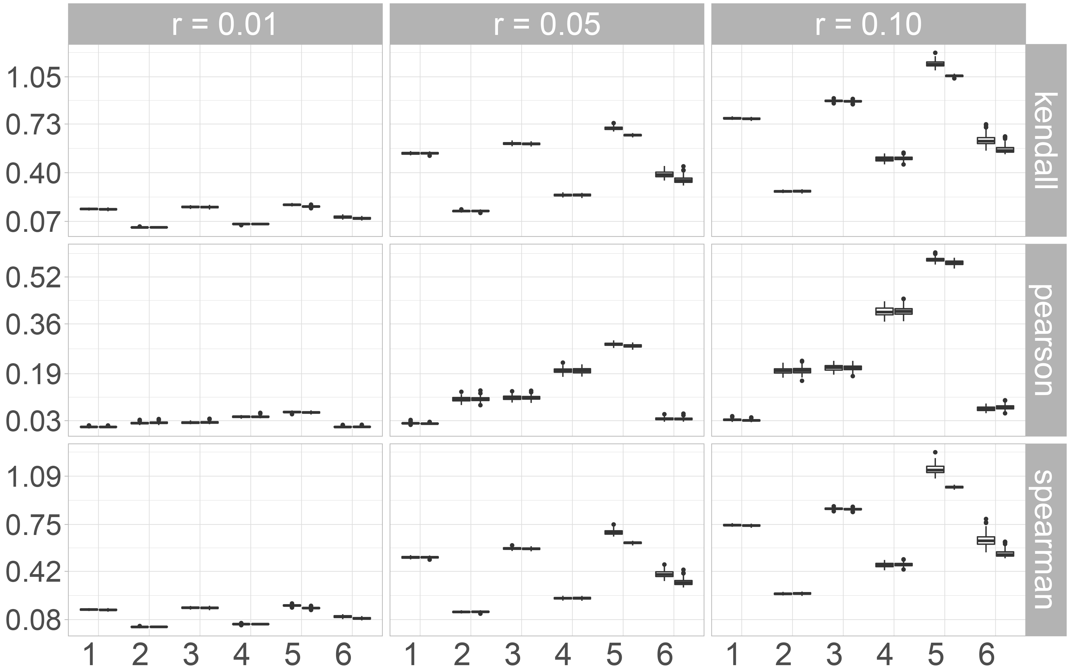Frobenius norm of the differences between the correlation matrices using $\text{𝑀𝐶}=100$ simulation runs. Each boxplot pair corresponds to the following missing mechanism: the left one to the MCAR, and the right one to the MAR mechanism. 1: Amelia, 2: Mice.Norm, 3: Mice.Pmm, 4: Mice.RF, 5: Naive, 6: missRanger.

For the simulations we use the pre-processed campus file data set described in Section 2.1. In our study, we first insert missing values into 24 previously selected variables (15 metric and 9 categorical) blackfrom the 28 variables of the data set, see also [3, 8] for further details. After inserting missing values, we impute the incomplete data set with the methods described in Section 2.2. For each imputed data set, we then calculate the evaluation measures as described in Section 3. In case of MICE we use different methods for the metric and categorical variables of our data set. For metric variables we use the options norm (Bayesian imputation under the normal linear model), pmm (predictive mean matching) and rf (random forest based imputation). For categorical variables only rf is applicable and used. In the following evaluation, the different methods are labeled by Mice.Norm, Mice.Pmm and Mice.RF. Strong dependencies between variables can result in computational difficulties when applying the imputation methods. Since strong dependencies are present for some metric variables in our data set, we restrict the selection of the potential covariates to those metric variables, which have a pairwise Pearson-correlation smaller than $0.8$ . The covariates can be specified by using the predictorMatrix-option in the mice-function of R. We made use of parallel computing for the MICE and the Amelia procedure. For Amelia, this was conducted by using the parallel option in the Amelia-function and for MICE we used the micemd package [23]. For the multiple imputation, we averaged the corresponding distance measures obtained from the $m=$ 5 imputed data sets.

Figure 2.

Pair of boxplots for the values for the 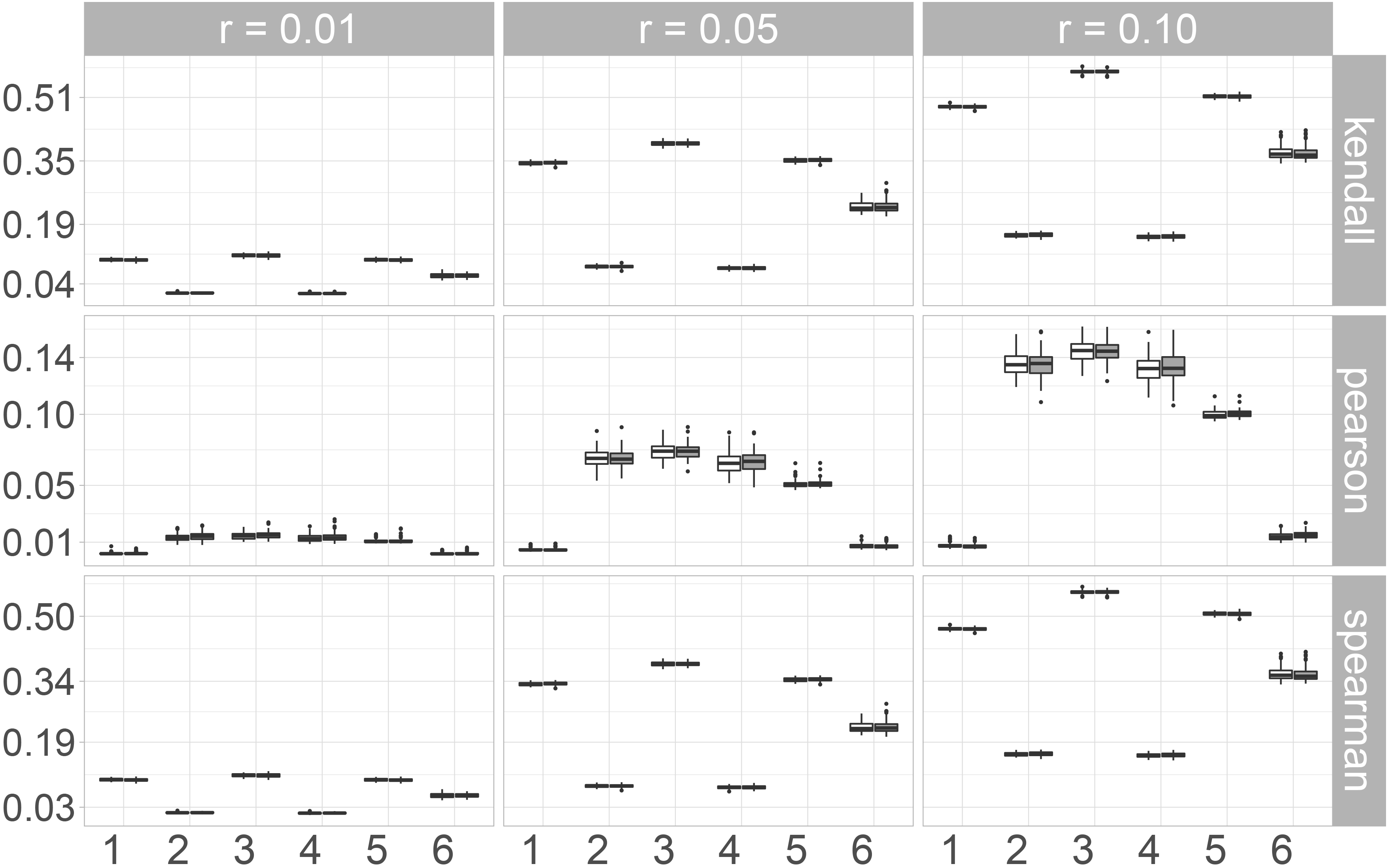Maximum norm of the differences between the correlation matrices using $\text{𝑀𝐶}=100$ simulation runs. Each boxplot pair corresponds to the following missing mechanism: the left one to the MCAR, and the right one to the MAR mechanism. 1: Amelia, 2: Mice.Norm, 3: Mice.Pmm, 4: Mice.RF, 5: Naive, 6: missRanger.

Each simulation setup consists of one missing rate $r\in \{0.01,0.05,0.1\}$ , and a missing mechanism (MAR and MCAR). We use the function prodNA for both missing mechanisms. Since we apply the MAR mechanism on three of the variables (Section 2.1), this results in an overall MAR mechanism. A detailed explanation of the dependence structure for inserting missing values under the MAR-mechanism and the implementation can be found on pages 14–16 in the Supplement of the arXiv preprint [8] as well as in [3]. For each simulation setup, we performed $100$ Monte-Carlo simulation runs.

4.2 Correlation coefficients

To assess (multivariate) distributional accuracy, we first consider the norms of the differences between the correlation matrices of the original and the imputed data sets. Here we distinguish between the Kendall, Pearson and Spearman correlation coefficients.

When taking a look at the Frobenius norm (Fig. 1), some differences between the three correlation coefficients can be observed. The results for the rank-based correlation coefficients Kendall’s $\tau$ and Spearman’s $\rho$ are similar to each other. For Pearson’s $r$ , the results differ. While Mice.Norm performs best for Kendall’s $\tau$ and Spearman’s $\rho$ , for Pearson’s $r$ , Amelia and missRanger perform better and even Mice.Pmm is just slightly worse than Mice.Norm. For Pearson’s $r$ , the lowest values (for all missing rates) can be observed when Amelia is used for imputation. But the observed values for missRangers are also very low and increase only slightly more than those of Amelia. For all correlation coefficients, the observed differences increase with increasing missing rate and the largest values can be observed for the Naive imputation. Additionally, for the Naive imputation and missRanger, small differences between the missing mechanisms can be observed for Kendall’s $\tau$ and Spearman’s $\rho$ . For both, imputation methods and correlation coefficients, the values for the MAR mechanism are slightly smaller than for the MCAR mechanism.

In Fig. 2 the boxplots for the Maximum norm are shown. For Kendall’s $\tau$ and Spearman’s $\rho$ , the results are similar to the Frobenius norm. The differences between the imputation methods only increase when looking at the Maximum norm instead of the Frobenius norm. When considering Pearson’s $r$ , the differences from the previous results are much larger. While for the Frobenius norm the highest values could be observed for the Naive Imputation, for the Maximum norm, the values for the three Mice algorithms are even slightly larger. Here, some of the correlations between the variables are reproduced more poorly by the Mice algorithms compared to the Naive imputation. However, on average the MICE procedures perform better than the Naive Imputation. Apart from this, the best values for the differences for Pearson’s $\rho$ can again be observed when using Amelia or missRanger. For Amelia the median value of the Maximum norm is even lower than 0.01. For missRanger, the median value is 0.014 for 10% missing values and the MAR mechanism and slightly larger in the MCAR case. Thus, it seems that all Pearson correlations between the variables can be reproduced reasonably well by these two algorithms. Turning to Kendall’s $\tau$ and Spearman’s $\rho$ , the best values can be observed when using Mice.Norm or Mice.RF with almost no differences between these two methods. The largest values can be observed for Mice.Pmm. This is a difference to the results of the Frobenius norm, where this method performed much better. A reason might be that the missing values are imputed by observed values of the variable, which leads to ties in the imputed data set. This in turn results in larger differences between the correlation matrices of the original and the imputed data set for some cases.

4.3 Kolmogorov-Smirnov-Statistics for linear combinations

In our previous research [3], we assessed imputation accuracy by computing the $p$ -values of the KS-Statistics for the variables of the data set. Extending this to the multivariate case blackwe use the findings of Cramér and Wold, which say that two multivariate distributions are equal if and only if their linear combinations are equal, and consider the KS-Statistic of 1000 randomly generated linear combinations of the variables.

In Fig. 3, the boxplots of the maximum values of the KS-Statistics of the 1000 linear combinations are shown. Between the two missing mechanisms, no major differences can be observed. For all imputation methods, the observed values increase when the number of missing values increases. The smallest maxima can be observed for Mice.Norm and missRanger, the highest for the Naive imputation. Amelia and Mice.Pmm perform worse than Mice.Norm, but still better than Mice.RF and the Naive imputation. Moreover, the values for Mice.Norm increase only a little with an increasing missing rate, while the increase is much higher for the other methods and especially for the Naive approach.

Figure 3.

Pair of boxplots for the 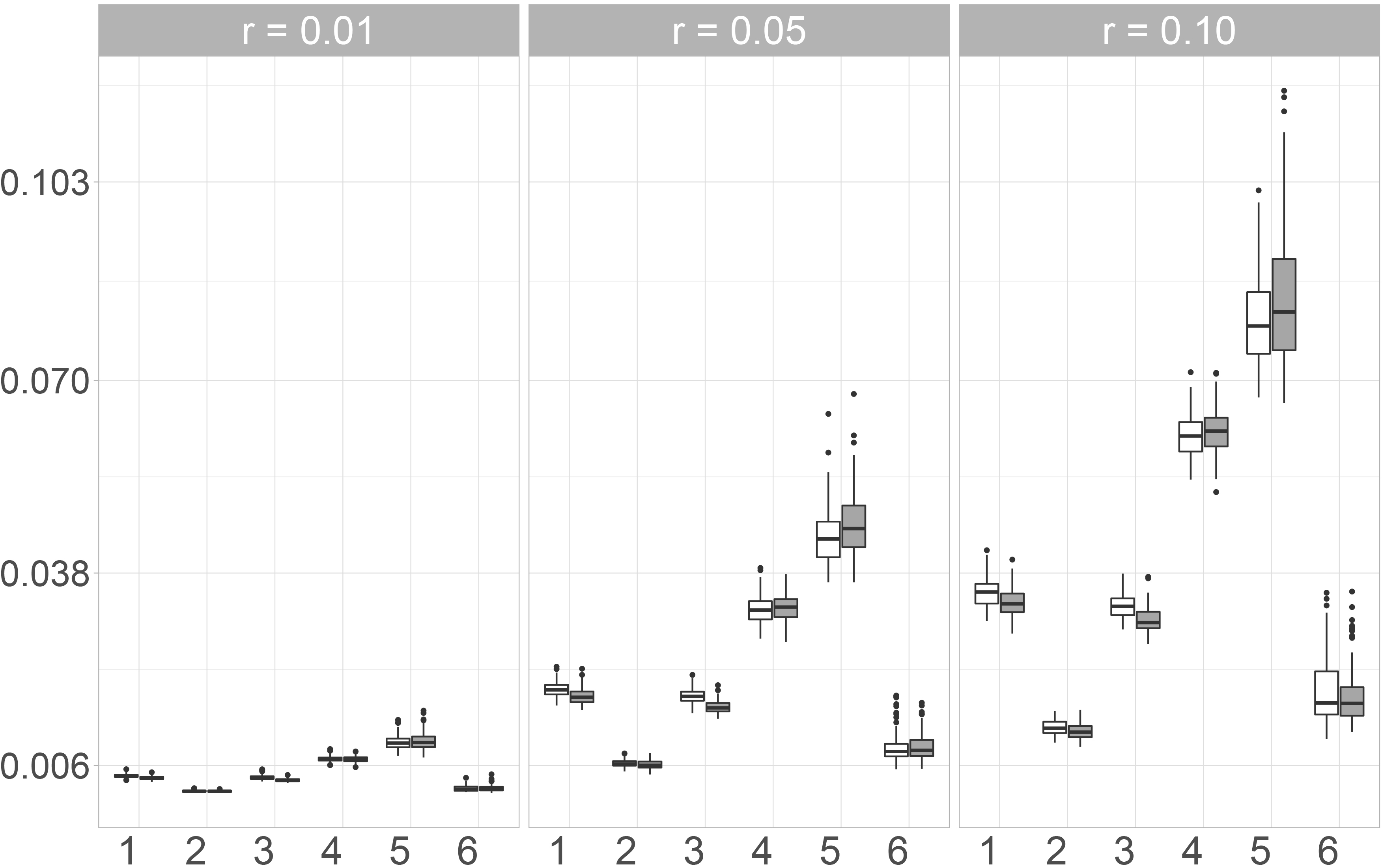maximum values of the Kolmogorov-Smirnov-Statistic for the linear combinations using $\text{𝑀𝐶}=100$ simulation runs and $B=1000$ linear combinations. Each boxplot pair corresponds to the following missing mechanism: the left one to the MCAR, and the right one to the MAR mechanism. 1: Amelia, 2: Mice.Norm, 3: Mice.Pmm, 4: Mice.RF, 5: Naive, 6: missRanger.

When looking at the arithmetic mean of the values for the 1000 linear combinations instead of the maximum, the differences between the naive imputation and the other imputation methods become even clearer. Again the smallest values can be observed for Mice.Norm and missRanger. Imputing missing values with the Amelia algorithm leads to similar results as using Mice.Pmm. Mice.RF only performs slightly worse than Mice.Pmm and Amelia. In fact, for a missing rate of 1%, the values for these three imputation methods only show small differences. This is contrary to the observations for the maximum value. Differences between the missing mechanisms can be observed for all imputation methods at a missing rate of 10 %. Here, the observed values are smaller when the missing values are simulated under the MAR-mechanism. For all imputation methods, the differences are again smaller for 1% and 5% missing values.

Figure 4.

Pair of boxplots for the 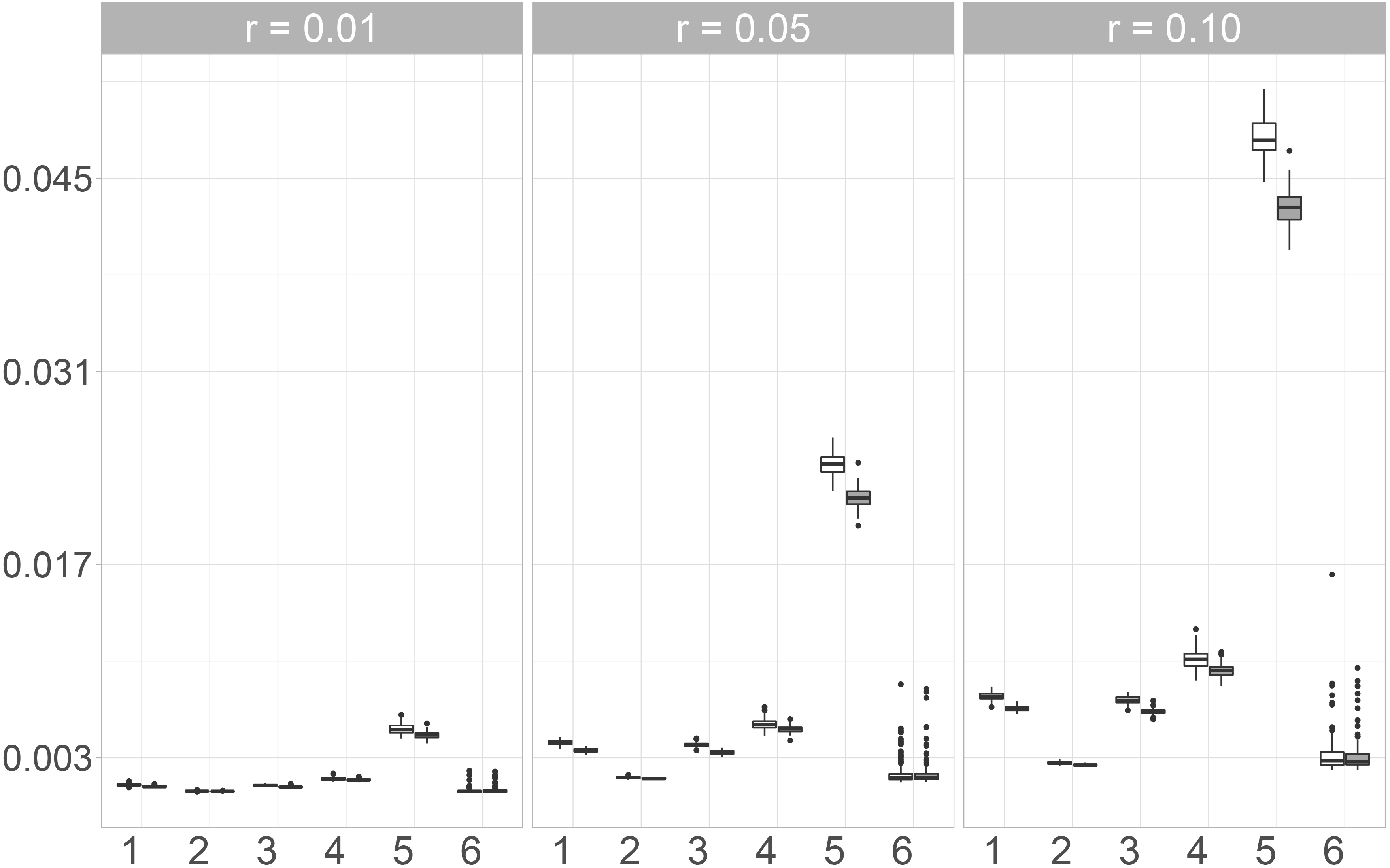mean values of the Kolmogorov-Smirnov-Statistic for the linear combinations using $MC=100$ simulation runs and $B=1000$ linear combinations. Each boxplot pair corresponds to the following missing mechanism: the left one to the MCAR, and the right one to the MAR mechanism. 1: Amelia, 2: Mice.Norm, 3: Mice.Pmm, 4: Mice.RF, 5: Naive, 6: missRanger.

4.4 Gaussian copula

We additionally consider the KS-Statistics of Copulas to assess multivariate distributional imputation accuracy. In our simulation, we considered three different Copulas. Since we could only observe small differences between these three, only the results for the Gaussian Copula are presented and displayed in Fig. 5.

Here, Mice.Norm exhibits the best performance while the largest values are observed for the Naive imputation. The variability of the observed values for the imputation with Amelia, Mice.Pmm and the naive method is almost the same, but the median values of Amelia and Mice.Pmm are much lower than when imputing missing values by using the Naive approach. The observed values for Mice.Norm show very low variability and also increase only slightly with an increasing missing rate. Additionally, the observed values for Mice.Norm are the lowest. Moreover, the differences between the two random forest approaches, Mice.RF and missRanger are not as big as for the other measures considered in this paper. When using the differences between the copulas as a measure for distributional similarity, Mice.RF performs slightly better than missRanger, since the median value and the variability of the values observed for Mice.RF are lower for the three missing rates.

Figure 5.

Pair of boxplots for the values of the 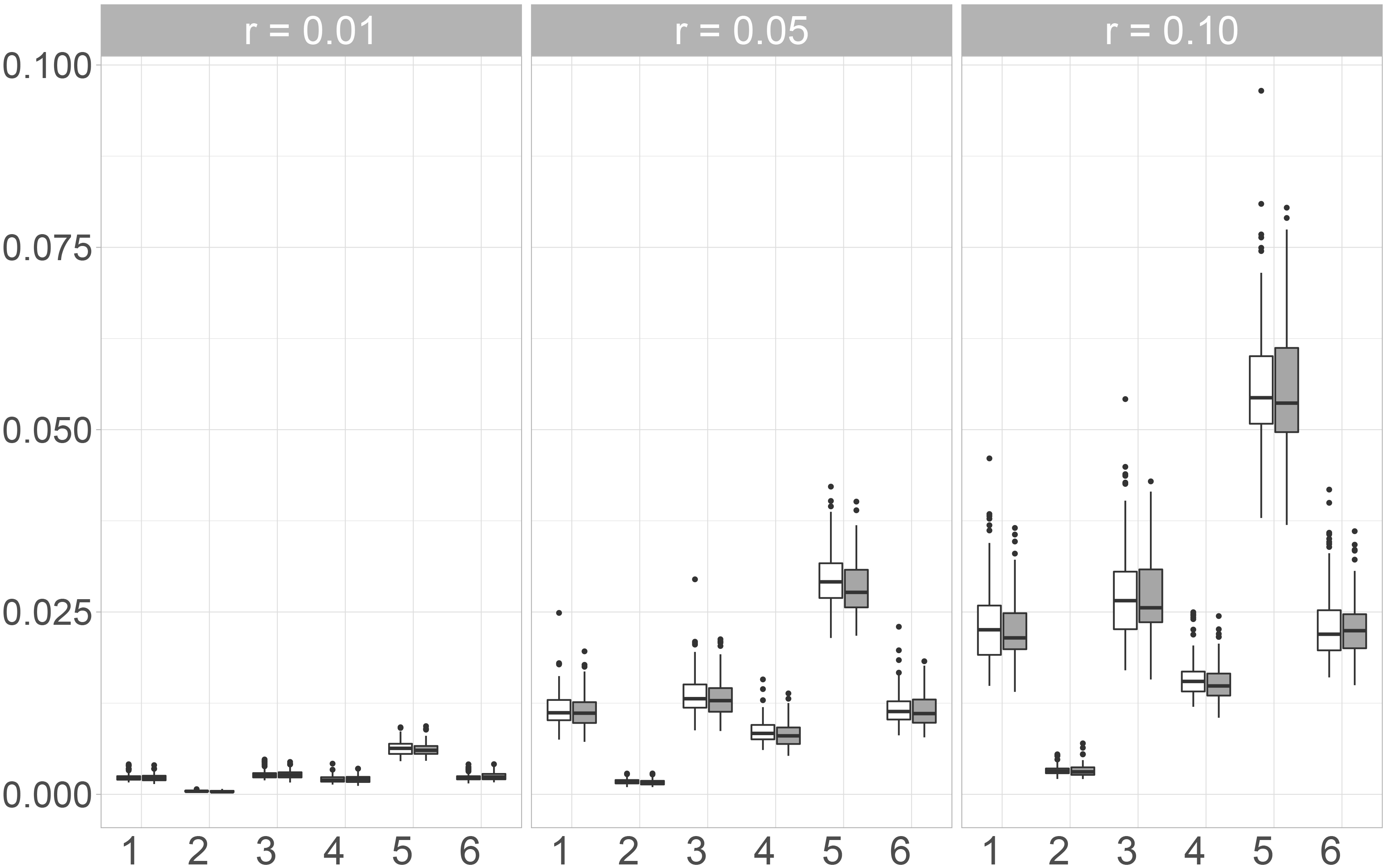Kolmogorov-Smirnov-Statistic of the estimated multivariate distribution functions of the original and imputed data set, estimated by the Gaussian Copula and using $B=10000$ bootstrap samples and $\text{𝑀𝐶}=100$ simulation runs. Each boxplot pair corresponds to the following missing mechanism: the left one to the MCAR, and the right one to the MAR mechanism. 1: Amelia, 2: Mice.Norm, 3: Mice.Pmm, 4: Mice.RF, 5: Naive, 6: missRanger.

4.5 Summary of the results

We compared six different imputation methods with respect to their (multivariate) distributional accuracy. This means that we were interested in the performance of the imputation methods in reproducing the multivariate distribution of the data generating process. The results for the KS-Statistics for the linear combinations and the Copulas are quite similar. The differences between the different correlation coefficients and between the Maximum and Frobenius norm are more pronounced. In fact, for the rank-based coefficients (Kendall’s $\tau$ and Spearman’s $\rho$ ) Mice.Norm performs best while Amelia and missRanger perform better when considering Pearson’s correlation coefficient. Thus, it seems that the imputation methods perform differently in reproducing monotone association respectively linear relations.

The results for the multivariate distributions (the KS-Statistics for the linear combinations and the Copulas) are slightly different to the results for the correlation coefficients. Here, Mice.Norm performs best for all three measures. Even for the maximum value of the KS-Statistic, where the variability of the observed values of some other imputation methods are really high (compared to the arithmetic mean of the values), the variation for Mice.Norm is rather small.

5. Discussion and outlook

5.1 Background

Imputation is known to be a powerful approach that allows for flexible subsequent analyses. However, for subsequent analyses to be trustworthy, one must be sure that the imputation procedures reflect the distribution of the underlying data generating process sufficiently well. This is especially true for problems involving multivariate features. This raises the question how well different imputation methods can reproduce correlations, associations or even the entire multivariate distribution. To give a first insight on this question we conducted a comparative simulation study for six state-of-the art imputation algorithms in which we assessed different aspects of their (multivariate) distributional accuracy. We therefore used the data set of the Structure of Earnings Survey 2010 which is provided as an anonymized data set by the Federal Statistical Office of Germany. In previous research [3], we already considered different measures to assess distributional accuracy. However, this previous analysis was restricted to univariate distributions and except for heuristic descriptive measures [24, 25, 26] or special methods that are based upon specific multivariate distributions [27, e.g.] we were not aware of other investigations in this direction.

5.2 Our approach

To assess multivariate distributional accuracy, we used the correlation coefficients of Kendall, Spearman and Pearson and compared the correlation matrices of the imputed data sets to the correlation matrix of the original data. For this comparison, we calculated the difference of the matrices and determined the Maximum and Frobenius norm. From this we analyzed how well the imputation methods preserve associations or relations between the variables. Our second approach to assess multivariate distributional accuracy was to compare the distributions of linear combinations of the variables of the data set before and after the imputation by calculating the Kolmogorov-Smirnov-Statistics of random linear combinations. In addition, we used copulas such as the Gaussian Copula to estimate the multivariate distributions of the data sets and evaluate the imputation accuracy with Kolmogorov-Smirnov-Statistics based thereon.

5.3 Our findings

The Naive imputation shows the worst performance of all approaches. Among the five other approaches, two stood out: Mice.Norm and the Random Forest based imputation missRanger. In particular, the latter performs well when considering the Frobenius or Maximum norm of the difference matrices of the Pearson correlation matrices and also exhibit good results in case of the KS-Statistic of the Gaussian Copula and the linear combinations. However, for these KS-type measures Mice.Norm performed the best and also showed very good results for most correlation measures considered in the simulation. Only for Pearson’s correlation, the observed values for the imputation with Mice.Norm are larger than for other imputation methods.

5.4 Limitations and outlook

While our study investigates various missing mechanisms, rates, and imputation methods, one limitation is that we only considered one dataset since the design of our simulation study is computationally very expensive. Moreover, we only considered distributional accuracy. Here, it would be of further interest to study in more detail how distributional accuracy effects other accuracy measures which, e.g. reflect inferential discrepancies as in [28] or differences in uncertainty quantification as in [29]. Therefore, additional studies (both theoretical and simulative) are needed in future research.