
Abstract
With the rapid proliferation of social data, the prevalence of missing values has become increasingly common. Various factors, including human error and machine failure, contribute to the emergence of missing values in datasets. Datasets containing missing values not only consume storage space but also pose a significant obstacle to direct utilization, resulting in substantial resource wastage. Consequently, accurately imputing missing values has emerged as a focal point in research. Generative missing value imputation methods, leveraging generative models, have demonstrated notable efficacy in recent years by directly generating values for missing components based on observable data values. This paper introduces a novel generative method for missing value imputation based on a diffusion denoising model, termed the conditional diffusion model for missing value imputation (CDMVI). Specifically, CDMVI trains a conditional diffusion model using complete data samples (samples devoid of missing values) and subsequently utilizes the trained model to impute missing values in datasets. During the training stage (i.e., the forward process of the diffusion model), a subset of features is randomly selected from complete data samples, and varying levels of random noise are introduced as condition inputs to the noise predictor within the diffusion model. In the imputation stage (i.e., the backward process of the diffusion model), the missing segments of the data are initially replaced with random noise, serving as a guide for the diffusion model to generate complete samples. Experimental evaluations across multiple datasets demonstrate the competitive performance of our proposed CDMVI method.
Introduction
The significance of data quality in contemporary artificial intelligence is paramount, as it directly influences the efficacy of model training. In practical scenarios, the pervasive issue of missing values remains a common hindrance to data quality. The presence of missing values can be attributed to a variety of factors, including human errors, machine malfunctions, and other unforeseen circumstances (Baraldi & Enders, 2010). For instance, in the context of recording medical data, inaccuracies due to operator errors might hinder the recording of a patient’s blood pressure, or the omission of sensitive information could result from the imperative of safeguarding patient privacy. These diverse reasons collectively contribute to the emergence of missing values in the final dataset (Ibrahim et al., 2012). Failing to address the challenge of missing values can obstruct the resolution of problems reliant on such data, potentially leading to unforeseeable losses. As a result, recent research endeavors have been dedicated to addressing the predicament of missing values. Among the proposed solutions, imputing the missing parts emerges as the most rational approach, minimizing any wastage of crucial data. Numerous researchers have introduced and developed distinct missing value imputation techniques from various perspectives. The overarching principle revolves around judiciously estimating the distribution of missing values and predicting reasonable fill-in values, ensuring that the imputed samples align with the overall data distribution (Dong & Peng, 2013).
In recent years, various methods for imputation of missing values have been proposed. According to the literature (Jarrett et al., 2022), existing methods for imputation of missing values can be roughly divided into two categories: iterative methods and deep generative models-based methods. Iterative methods hinge on estimating the conditional distribution of a feature by utilizing all other available features. In each iteration, a conditional distribution estimator is trained to predict the value of each feature. This single-variable model is then employed recursively to impute missing values until the process converges, guided by a prespecified convergence criterion (Zheng & Charoenphakdee, 2022). This method has undergone extensive study and application (Khan & Hoque, 2020; Stekhoven & Bühlmann, 2012), with multiple imputation using chain equations (MICE; Van Buuren & Oudshoorn, 2000 standing out as one of the most renowned techniques. The MICE algorithm predicts missing values in a feature by establishing equations between the single feature and other observed features. It utilizes the predicted missing values as known variables to further predict the missing values in another single feature. Through iterative execution of these steps, the MICE algorithm converges to obtain the final imputed values for the missing part. On the other hand, missing value imputation methods based on deep generative models operate by estimating the joint model of all features. By training a generative model, these methods generate plausible values for the missing part based on observed values (Li et al., 2019; Rezende et al., 2014). According to the characteristics of the generative model, Yoon et al. (2018) proposed the generative adversarial imputation nets (GAIN), The core idea behind GAIN is to generate estimates of the missing part using a generator and employ a discriminator to assess the disparity between the generated estimates and the actual values. This iterative optimization process refines both the generator and discriminator, ultimately yielding a more accurate imputation result for the missing data. Simultaneously, Gondara and Wang (2018) proposed multiple imputation using denoising autoencoders (MIDA) for missing value imputation. The MIDA model adopts a self-encoder architecture (Wang et al., 2016) and introduces noise to the input to enhance the model’s ability to reconstruct the original input from noisy data. Subsequently, Nazabal et al. (2020) proposed a missing value imputation model called HIVAE, which uses variational autoencoders (VAEs) as the main architecture. Other methods for imputation of missing values based on generative models include (Dai et al., 2021; Li et al., 2019; Yoon & Sull, 2020).
In recent times, diffusion models (Cao et al., 2022; Chen et al., 2023; Yang et al., 2023), emerging as a noteworthy class of generative models, have demonstrated their effectiveness across diverse domains, including computer vision (Ho et al., 2020), time series data (Rasul et al., 2021), and natural language processing (Li et al., 2022). When compared to other generative models, diffusion models have exhibited notable prowess. These models incrementally introduce noise to the data through the forward process and systematically denoise the random Gaussian noise during the backward process to generate samples. Despite their demonstrated efficacy in various applications, diffusion models, as a relatively novel generative model, have seen limited exploration in the context of addressing the challenge of missing value imputation.
In this study, we introduce a diffusion-based framework, referred to as conditional diffusion model for missing value imputation (CDMVI), designed for the imputation of missing values in data. Specifically, CDMVI employs a diffusion model trained on complete samples (i.e., samples without missing values) to capture the original distribution of the data. In the forward process of the diffusion model, we systematically introduce random Gaussian noise to complete samples, generating perturbed samples. Concurrently, we implement distinct masking strategies to simulate missing values in the data. We input samples with missing values and perturbed samples with noise into a U-shaped network to predict the amount of noise added to the samples. Here, the samples with missing values serve as a conditioning factor for the diffusion model, enhancing the U-shaped network’s accuracy in predicting the noise added during the forward process. In the backward process of the diffusion model, we utilize random Gaussian noise and real samples with missing values as inputs. After multiple denoising iterations, complete samples corresponding to the samples with missing values are obtained. Consequently, we refer to the backward process as the missing value-filling process. Our contributions can be summarized as follows:
We introduce a framework, CDMVI, based on the conditional diffusion model, tailored for generative missing value imputation, with a specific emphasis on numerical data and multiple missing patterns. We design a conditional generation model and seamlessly integrate the generated conditions into the noise predictor within the diffusion model. This integration facilitates the denoising process in the direction of missing value generation. We conduct extensive numerical experiments on various real datasets under different missing mechanisms, demonstrating the efficacy of CDMVI in effectively addressing missing value imputation challenges.
Related Work
Missing Data
Dealing with missing values is a prevalent challenge in both data analysis and machine learning. This pertains to the presence of unobserved or invalid values within a dataset. Such missing values can arise due to various factors, including measurement errors, problems during data acquisition, intentional data gaps, or issues related to data quality. Table 1 illustrates scenarios where missing values are encountered in the dataset, with these instances being represented by the symbol “?.”
Missing Value Display.
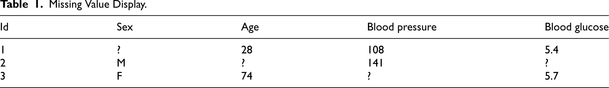
Missing Value Display.
Missing data can be broadly categorized into three types: missing completely at random (MCAR), missing at random (MAR), and missing not at random (MNAR; Purwar & Singh, 2015). MCAR denotes missing data that is independent of both itself and other variables, meaning the occurrence of missing values for a variable is entirely random. For instance, in a street survey, participants may drop out midway for various reasons, resulting in incomplete data. Such missing values are considered completely random (Jerez et al., 2010). Handling MCAR is relatively straightforward, as missing values can be directly deleted without introducing estimation bias. Alternatively, appropriate filling methods can be applied to maximize the utilization of sample information, though this approach may result in some loss of data. On the other hand, MAR describes situations where data is missing in connection to other observable variables. For instance, in a test scenario, individuals failing to meet the minimum intelligence quotient requirement of 100 points may be excluded from subsequent personality tests. Here, missing values not only lead to information loss but can also introduce bias into the analysis results. Dealing with MAR requires more sophisticated techniques than MCAR, as directly deleting or filling missing values with averages may not be suitable (Cummings, 2013). Although MAR is more complex than MCAR, it is a more commonly encountered scenario. MNAR implies that missing data is only related to the variable itself. For example, in a company that recently hired 20 employees, six were dismissed during the probation period due to poor performance. In the subsequent performance evaluation after the probation period, the performance scores of the dismissed employees are missing (Bertsimas et al., 2018).
Missing Value Filling Method
Various effective techniques have been developed for addressing missing values, and in the subsequent discussion, we provide a brief overview of the current landscape of methods in this domain. We delve into several algorithms for comparison, exploring their relationships and offering our recommendations. One of the most widely used imputation methods is class mean imputation, where the entire sample is categorized into classes based on weighted classes derived from auxiliary variables. Within each imputation category, missing responses are imputed with the average value of the corresponding class. Despite its common usage, this method may introduce bias in estimating variance and covariance. Sensitivity to extreme values can compromise average calculations. The random imputation method involves selecting a respondent at random from the imputation category to fill in the missing value. While cost-effective and easy to implement, it tends to underestimate standard errors, leading to an overestimation of test statistics. Regression imputation predicts the missing value by establishing a regression equation with other variables. Although it may incur high computational costs, particularly with datasets featuring numerous variables, it remains a viable option. The k nearest neighbor (kNN) imputation method (Liu et al., 2015) employs values computed from the kNN observations to fill in missing data. It identifies the kNNs of a new data point in the feature space and predicts the missing value based on the attribute values of these neighbors, using measures such as average, median, or mode. Support vector machine and support vector regression are well-established learning-based missing value imputation techniques, catering to discrete/classification and continuous/numerical missing data imputation, respectively. These techniques utilize a kernel function to map the original feature space nonlinearly to a high-dimensional feature space, constructing a hyperplane for linear separation of data samples in the new feature space (Byun & Lee, 2003). Recently, there has been a surge in applying deep learning techniques to missing value imputation challenges. This includes methods leveraging graph neural networks (Zhong et al., 2023), diffusion models (Zheng & Charoenphakdee, 2022), or VAEs (Mattei & Frellsen, 2019). These techniques, with their nonlinear computation capabilities, prove adept at uncovering intricate correlations within data.
Method
Problem Definition
Let data matrix
Denoising Diffusion Probabilistic Models
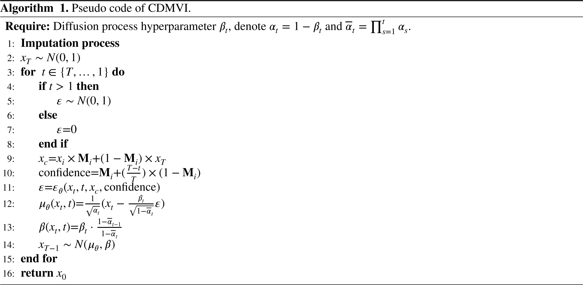
This article employs the conditional diffusion model (Dhariwal & Nichol, 2021) as a generative method for the restoration of missing values in data. Similar to other generative models, the diffusion model discerns the distribution of training data through specific training methods. The fundamental concept behind the diffusion model involves systematically perturbing the structure within the data distribution using a forward Markov process. Subsequently, the model learns a backward process to recover this perturbed structure, resulting in a highly flexible and easily manageable generative model. During the training phase of the diffusion model, the forward process remains fixed, and the focus lies solely on training its backward process.
During the training process, the diffusion model defines a diffusion process that converts the sample 


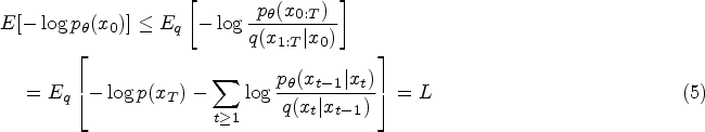
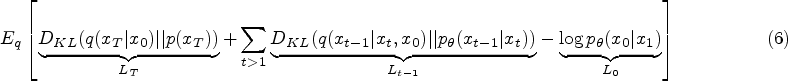


Traditionally, the training of the diffusion model involves instructing an Unet, also referred to as the noise predictor, to forecast the noise introduced to the samples. This Unet takes the sample 


The framework of our proposed conditional diffusion model for missing value imputation (CDMVI).
By minimizing the error between the predicted noise and the actual noise of the sample, we can train the parameters in the model 
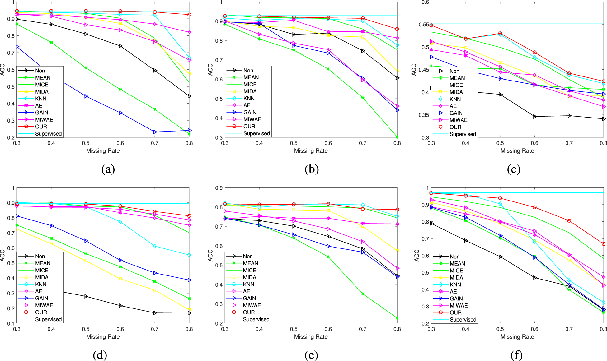
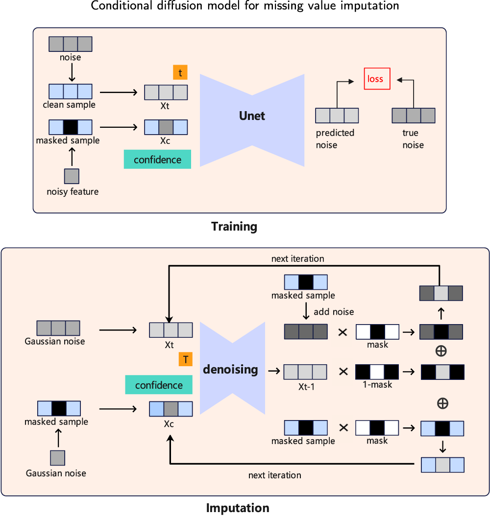
Classification performance of different missing rates: (a) USPS, (b) MNIST, (c) First-order, (d) Satimage, (e) Fashion, and (f) Optdigits datasets.
After predicting the noise, we can obtain the mean and variance of 
In this section, we perform an extensive set of experiments to assess the effectiveness of our proposed method. Initially, we evaluate multiple aspects of CDMVI using the USPS dataset. We qualitatively showcase the behavior of CDMVI across diverse missing patterns and architectural variations. Subsequently, we compare CDMVI against various baseline methods in the context of missing data imputation. This comparative analysis is conducted across six datasets, encompassing a spectrum of missing settings.
Datasets
In this paper, we evaluated CDMVI on six datasets that are widely used in machine learning and data science. These datasets have different characteristics and uses, covering different fields and problems. For all datasets, the feature value range of each sample was rescaled to MNIST dataset: MNIST is a large dataset containing handwritten digits that are commonly used to train image processing systems. The dataset contains 60,000 training samples and 10,000 test samples, each of which is a Fashion-MNIST dataset: Fashion-MNIST is an image dataset that replaces the MNIST handwritten digit set. It covers 70,000 different product front images from 10 categories, with 7000 USPS dataset: The USPS dataset is a handwritten digit image dataset that contains a large number of handwritten digit images and corresponding labels. Each image in the USPS dataset is a First-order dataset: The content of the first-order dataset is given in a theorem to predict which of the five heuristics will give the fastest proof when used by a first-order prover. If the theorem is too difficult, the sixth prediction rejects the attempt to prove it. The dataset contains 6120 samples, each with 51 features, and all samples can be divided into six categories. Satellite image dataset: The dataset consists of multispectral values of pixels in a Optdigits dataset: The optdigits dataset contains 5620 samples, each of which contains 64 features, from 10 categories in total.
Comparison With Related Methods
Mean: The basic idea of this method is to use the average of other values in the dataset to fill in missing values. Specifically, for a set of samples containing missing values, calculate the average of each feature excluding the missing values, and replace the missing part with the average value corresponding to each feature as the fill value.
MICE (Zhang, 2016): It is constructed based on multiple imputation methods. For a variable with missing values, data from other variables are used to fit the variable, and the fitted prediction values are used to fill in the missing values of the variable.
MIDA (Gondara & Wang, 2018): We propose a multi-imputation framework based on a fully supervised denoising autoencoder model, in which we simulate multiple predictions by initializing our model with a different set of random weights at each run.
kNN (Zhang, 2012): It first finds the kNNs of any case based on the similarity between cases, and then fills in missing values by setting function values (such as mean, median, mode, etc.) in these nearest neighbor cases
Autoencoder (AE; Ng et al., 2011): During the encoding stage, the AE encodes the input data into a low-dimensional representation, often learning effective features of the data. During the decoding stage, the AE decodes the low-dimensional representation back into the original data space, generating a complete output with no missing values.
GAIN (Yoon et al., 2018): In GAIN, there is a generator and a discriminator. The generator is responsible for generating new data samples, while the discriminator is responsible for determining whether these generated data samples are similar to real data samples. First, the generator generates a fill-in value for each missing value. Then, the discriminator judges whether this fill-in value is similar to the true value. If it is similar, then this fill-in value will be retained; if not, it will be returned to the generator for adjustment.
Missing data importance weighted autoencoder (MIWAE; Mattei & Frellsen, 2019): The MIWAE model is a generalized version of the IWAE. IWAE is a generative model with the same architecture as the VAE, which introduces an importance-weighted strategy to optimize the objective function of the VAE. In IWAE, the encoder model uses multiple samples to approximate the posterior, which is more flexible for modeling complex posteriors. Unlike IWAE, the objective function of MIWAE only focuses on the observed part with single-value filling. Finally, the missing values of the original matrix
Evaluation Metrics
The sum of the root mean square error (RMSE) calculated using each attribute on the test set is compared, and the calculation result is,
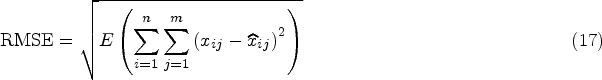
We conducted a total of 10 experiments, each comprising five cross-validation trials, wherein we employed RMSE as the performance metric. To illustrate the impact of filled features in machine learning tasks, we further conducted classification tasks on the samples with filled features. This involved utilizing supervised training classification models to assess classification accuracy. Default settings from respective papers were adhered to for all baseline methods. The datasets were partitioned into an 80% training subset and a 20% test subset. For missing value-filling algorithms necessitating training (e.g., GAIN, MIWAE, and CDMVI), the model underwent training on the training set. Subsequently, values of features in the test set were randomly deleted, and the trained model was then validated on the test set. In contrast, algorithms not requiring training (e.g., Mean, MICE, and kNN) had the training set and test set concatenated as input. During training, data feature values were scaled to
RMSE Results
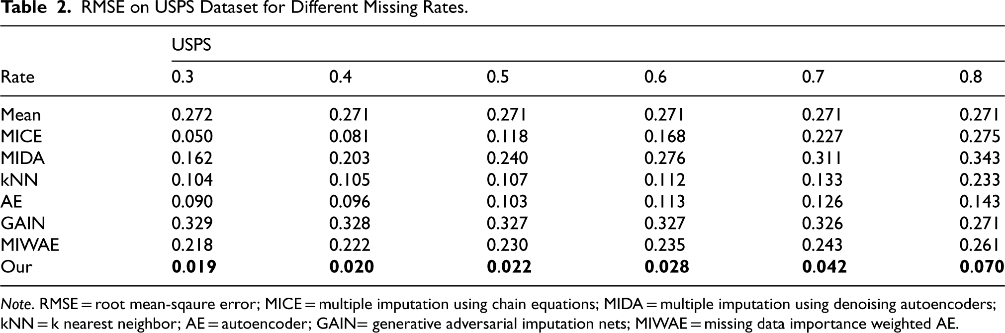
We employed six real datasets sourced from the UCI machine learning repository to quantitatively assess the performance of our method in terms of imputation accuracy. Tables 2 to 7 present the RMSE values of CDMVI alongside seven baseline methods, with the optimal outcomes highlighted in bold. Across the six tables, it is evident that all methods exhibit a decline in performance as the missing rate increases. Notably, our method consistently outperformed other approaches in the majority of cases. Specifically, for the six datasets spanning varying missing rates, the average RMSE values for our method were 0.034, 0.125, 0.070, 0.058, 0.114, and 0.178, respectively. In comparison to alternative methods, our approach reduced RMSE by 0.078, 0.016, 0.007, 0.003, 0.003, and 0.014 across the six datasets when compared to the best-performing method. When contrasted with the least effective method, our approach achieved RMSE reductions of 0.284, 0.133, 0.087, 0.216, 0.184, and 0.122 on the respective datasets. Several factors contribute to the superior performance of our method. Firstly, diffusion-based methods effectively learn data distributions and generate values that align with the missing parts distribution. Secondly, observable feature values provide conditional guidance for the diffusion process, enhancing the accuracy of generated values for missing data. Thirdly, our method leverages the numerical values of missing parts obtained at each step of sample denoising as additional information, contributing to its efficacy.
RMSE on USPS Dataset for Different Missing Rates.
RMSE on USPS Dataset for Different Missing Rates.
Note. RMSE = root mean-sqaure error; MICE = multiple imputation using chain equations; MIDA = multiple imputation using denoising autoencoders; kNN = k nearest neighbor; AE = autoencoder; GAIN= generative adversarial imputation nets; MIWAE = missing data importance weighted AE.
RMSE on MNIST Dataset for Different Missing Rates.
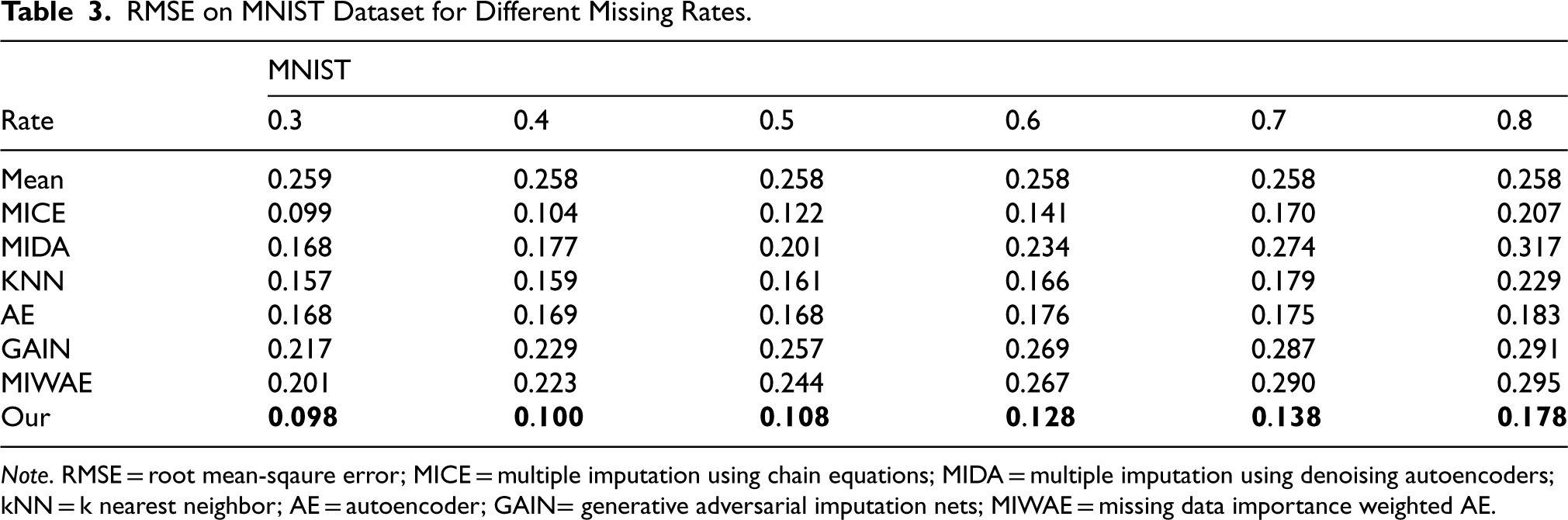
Note. RMSE = root mean-sqaure error; MICE = multiple imputation using chain equations; MIDA = multiple imputation using denoising autoencoders; kNN = k nearest neighbor; AE = autoencoder; GAIN= generative adversarial imputation nets; MIWAE = missing data importance weighted AE.
RMSE on First-Order Dataset for Different Missing Rates.
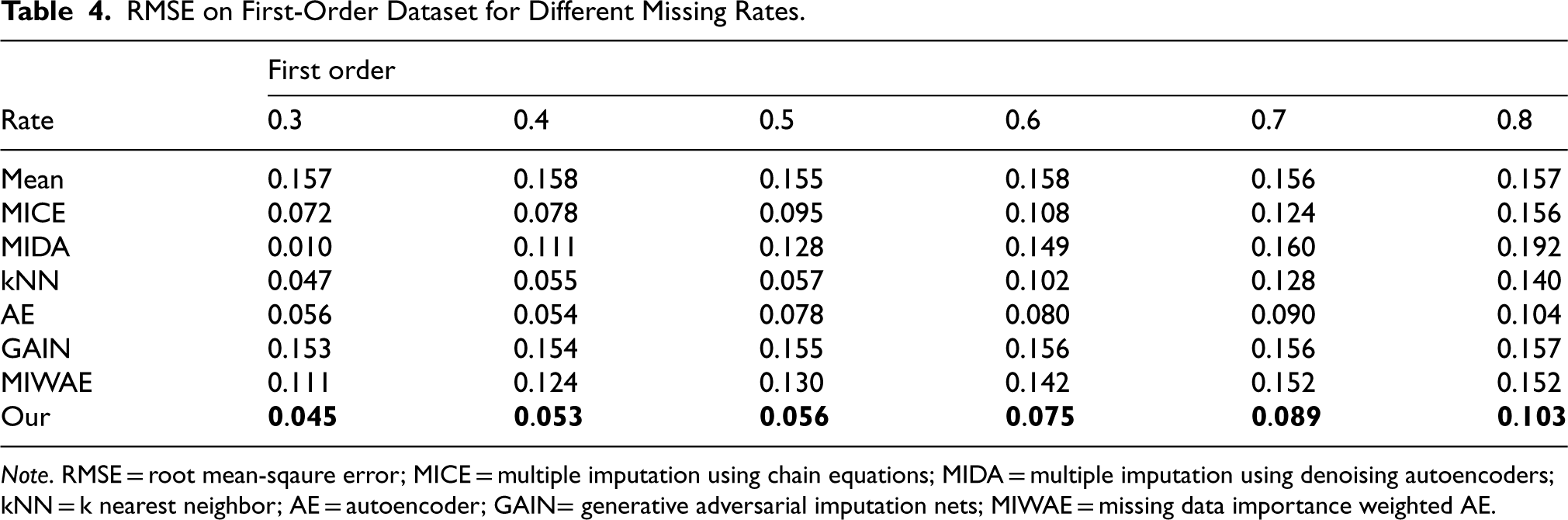
Note. RMSE = root mean-sqaure error; MICE = multiple imputation using chain equations; MIDA = multiple imputation using denoising autoencoders; kNN = k nearest neighbor; AE = autoencoder; GAIN= generative adversarial imputation nets; MIWAE = missing data importance weighted AE.
RMSE on Satimage Dataset for Different Missing Rates.
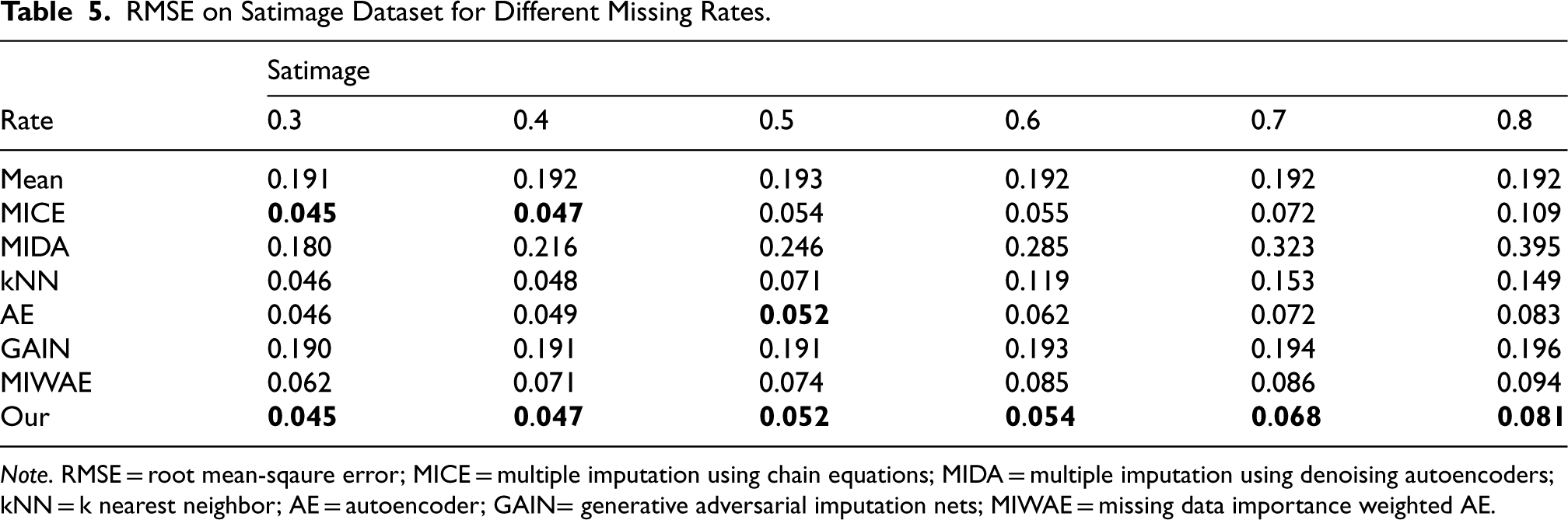
Note. RMSE = root mean-sqaure error; MICE = multiple imputation using chain equations; MIDA = multiple imputation using denoising autoencoders; kNN = k nearest neighbor; AE = autoencoder; GAIN= generative adversarial imputation nets; MIWAE = missing data importance weighted AE.
RMSE on Fashion Dataset for Different Missing Rates.
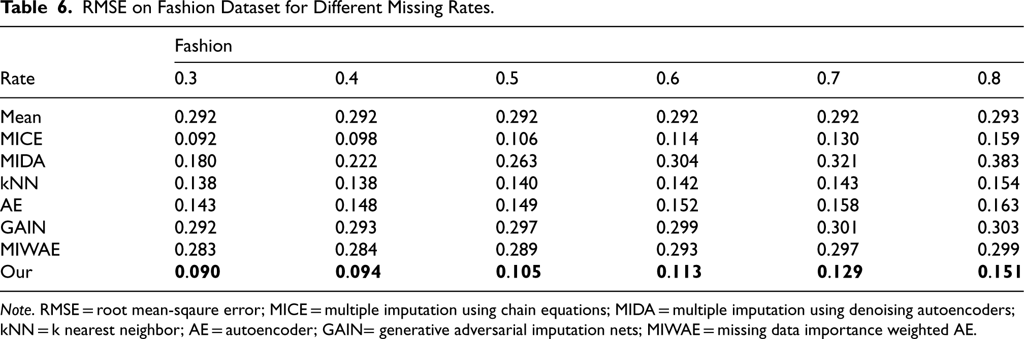
Note. RMSE = root mean-sqaure error; MICE = multiple imputation using chain equations; MIDA = multiple imputation using denoising autoencoders; kNN = k nearest neighbor; AE = autoencoder; GAIN= generative adversarial imputation nets; MIWAE = missing data importance weighted AE.
RMSE on Optdigits Dataset for Different Missing Rates.
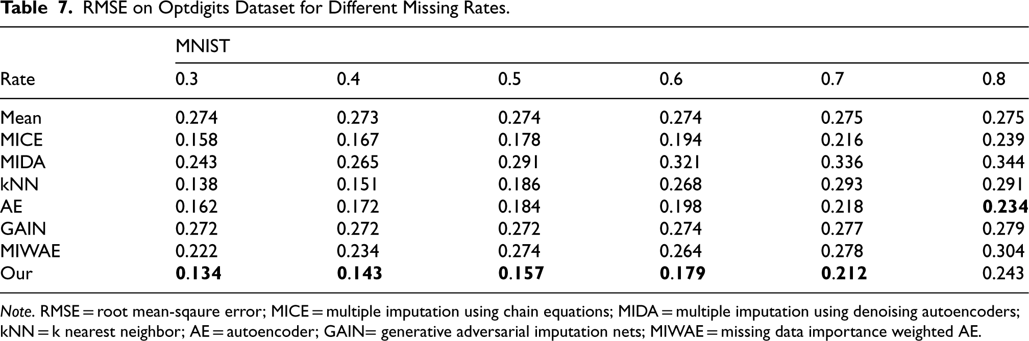
Note. RMSE = root mean-sqaure error; MICE = multiple imputation using chain equations; MIDA = multiple imputation using denoising autoencoders; kNN = k nearest neighbor; AE = autoencoder; GAIN= generative adversarial imputation nets; MIWAE = missing data importance weighted AE.
In addition to calculating the RMSE for the filled values, we explored the use of the filled samples for downstream tasks to more intuitively showcase the effectiveness of the imputed values. We selected classification tasks as the downstream applications following the imputation. All six datasets chosen for this analysis have ground truth labels for classification. The following steps were undertaken to obtain and compare the classification results: First, we simulated missing values of the MCAR type with varying missing rates. Subsequently, estimation methods were employed to fill the datasets with missing values. Next, complete samples were utilized as the training set to train a classifier, with the filled samples employed for testing and reporting the classification accuracy. Additionally, two baseline methods were included for reference: one utilizing the classification accuracy of real samples as a supervisory benchmark, and the other filling the missing part with zeros. This sampling process was iterated 10 times to conduct statistical analysis on the estimation methods.
Figure 2 illustrates the performance of all missing value imputation methods on classification tasks. It is evident from the figure that the classification accuracy of the complete dataset without missing values is intuitively the highest. While our method performs slightly below the classification accuracy of the complete dataset without missing values, it outperforms all other compared methods. Furthermore, as the missing rate in the sample increases, the classification accuracy of all missing value imputation methods in downstream classification tasks continues to decline. Specifically, our method achieved average classification accuracies of 0.940, 0.910, 0.492, 0.868, 0.806, and 0.869 on six datasets, respectively. In comparison to the classification accuracy of the complete sample, our method is lower by 0.005, 0.018, 0.059, 0.027, 0.010, and 0.101, respectively. Contrasting with the worst-performing method, our method is higher by 0.513, 0.260, 0.118, 0.606, 0.270, and 0.329, respectively.
Additionally, an intriguing observation is that some methods perform worse than 0-value filling on certain datasets, such as USPS, MNIST, and Fashion datasets. This phenomenon suggests that the values filled in the missing positions by these methods not only fail to enhance the performance of the samples in classification tasks but also impede the samples’ utility. Upon further investigation, we noted that datasets exhibiting this phenomenon are image data, leading us to speculate that incorrect filling values may impact the extraction of image semantics and hinder the model’s understanding of the image.
Qualitative Analysis
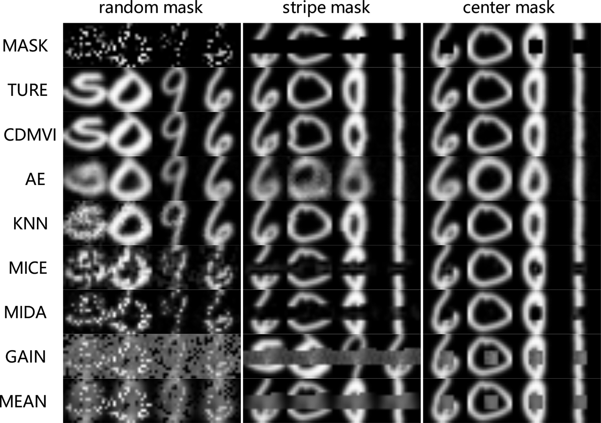
To visually illustrate the accuracy of our method in imputing missing values, we conducted a qualitative analysis of the visual outcomes across various techniques applied to the USPS dataset. We introduced three distinct types of missing values, including completely random missing, bar-shaped missing, and center-missing. The filling results of all methods were compared, as depicted in Figure 3. The visual inspection of the results clearly highlights the superior performance of our method in accurately filling in missing values across all three types of scenarios. Notably, the visual effects achieved by our method closely approach the completeness of the original image. This demonstration emphasizes the robustness and precision of our approach, showcasing its ability to generate visually clear and accurate imputations in diverse missing data patterns.
Breast.
We introduce a missing value imputation method, termed CDMVI. In this approach, we incorporate conditional guidance into the training of the diffusion denoising model to judiciously leverage the samples acquired at each denoising step. Extensive numerical simulations have been conducted, demonstrating the robust imputation performance of our method. Moreover, our results indicate that CDMVI achieves competitive performance compared to other well-established imputation methods. Future research directions may explore the design of alternative training strategies for the diffusion model to streamline the denoising process and enhance imputation accuracy for missing data segments.
Footnotes
Funding
The authors received no financial support for the research, authorship, and/or publication of this article.
Declaration of conflicting interests
The authors declared no potential conflicts of interest with respect to the research, authorship, and/or publication of this article.