Can Dopamine Responsiveness Be Predicted in Parkinson’s Disease Without an Acute Administration Test?

Abstract

Background:

Dopamine responsiveness (dopa-sensitivity) is an important parameter in the management of patients with Parkinson’s disease (PD). For quantification of this parameter, patients undergo a challenge test with acute Levodopa administration after drug withdrawal, which may lead to patient discomfort and use of significant resources.

Objective:

Our objective was to develop a predictive model combining clinical scores and imaging.

Methods:

350 patients, recruited by 13 specialist French centers and considered for deep brain stimulation, underwent an acute L-dopa challenge (dopa-sensitivity > 30%), full assessment, and MRI investigations, including T1w and R2* images. Data were randomly divided into a learning base from 10 centers and data from the remaining centers for testing. A machine selection approach was applied to choose the optimal variables and these were then used in regression modeling. Complexity of the modelling was incremental, while the first model considered only clinical variables, the subsequent included imaging features. The performances were evaluated by comparing the estimated values and actual values

Results:

Whatever the model, the variables age, sex, disease duration, and motor scores were selected as contributors. The first model used them and the coefficients of determination (R²) was 0.60 for the testing set and 0.69 in the learning set (p < 0.001). The models that added imaging features enhanced the performances: with T1w (R² = 0.65 and 0.76, p < 0.001) and with R2* (R² = 0.60 and 0.72, p < 0.001).

Conclusion:

These results suggest that modeling is potentially a simple way to estimate dopa-sensitivity, but requires confirmation in a larger population, including patients with dopa-sensitivity < 30%

INTRODUCTION

Dopamine replacement therapy is the first-line pharmacologic treatment for Parkinson’s disease (PD) [1]. Levodopa (L-dopa), an oral dopamine precursor combined with a peripheral dopa decarboxylase inhibitor, is the most commonly prescribed drug. It predominantly improves motor symptoms, particularly akinesia and rigidity by compensation for striatal dopamine depletion. The severity of these motor symptoms, related to the level of degeneration and dopamine depletion, differs from one patient to another. As a consequence, patients may exhibit different responses to L-dopa [2, 3]. This response is called dopa responsiveness or dopa-sensitivity.

Evaluation of dopa-sensitivity, consisting in measuring the contrast between the “ON” and “OFF conditions, usually requires an acute administration test in hospital after overnight withdrawal of treatment or even longer if the patient is receiving sustained-release dopamine agonists. This acute L-dopa challenge, in addition to having a real economic cost, is sometimes poorly tolerated by the patient during the “OFF” time, and is a burden for the evaluator. In addition, the acute effect may sometime differ from the chronic effect of L-dopa. Predictive modeling appears, thus potentially of interest to reduce these burdens. While this modeling was widely used in different applications as diagnosis and prognosis and employing several analytical methods [4], very few works focused on this issue. Two recent studies reported the first results towards this kind of approaches. In 2019, Khodakarami et al. [5] investigated the contribution of an ambulatory wearable device, the Parkinson’s Kinetigraph. They combined the measured features with the Unified Parkinson’s Disease Rating Scale Part III (UPDRS III) score in “ON” and “OFF” conditions to build a model of motor function severity levels, subsequently allowing predicting variations of Dopa-sensitivity. In 2021, Aman et al. [6], using data from the Levodopa response study of the Michael J. Fox Foundation for PD research, compared different demographic and clinical features between good responders and bad responders and examined several machine learning algorithms to build models allowing the best classification.

In this study, guided by the aim of building a non-invasive prediction model of patient individual dopa-sensitivity, we examined the combination of demographic data and “ON” condition clinical scores evaluating disease severity to produce such a model. MRI features were also investigated. It is now well established that this imaging modality, able to quantify brain degeneration, can be useful in PD. T2* weighted relaxometry and susceptibility-weighted mapping analyses derived from gradient multi-echo sequences can be used to quantify the iron load and nigral degeneration, characteristic of the disease [7, 8]. Anatomic imaging, using T1-weighted sequences, can indicate alterations in gray matter volume and cortical changes [9, 10].

METHODS

Study population and clinical data

Patients were enrolled prospectively in 13 specialist centers for movement disorders belonging to a national network (NS-PARK-F-CRIN) in France during their selection for sub-thalamic nucleus deep brain stimulation (DBS), as an ancillary study to the PREDISTIM study (Study of the predictive factors for therapeutic response of subthalamic stimulation on quality of life in Parkinson’s disease). The study was funded by the French Ministry of Health (PHRC-N) and the French charity, France Parkinson. It was approved by the local institutional review board (CPP Nord Ouest IV, Lille, France; study reference: 2013-A00193-42; identified under NCT02360683 in ClinicalTrials.gov). All participants provided their written, informed consent before taking part. The study complied with the methods, guidelines, and regulations described in the approved protocol.

All patients met the Movement Disorders Society (MDS) clinical criteria for the diagnosis of PD [11] and selection criteria for DBS: age < 75 years; disease duration > 5 years; no severe cognitive impairment or dementia with a Montreal Cognitive Assessment (MoCA) score < 24 and DSM-IV criteria; no parkinsonian psychosis or other severe psychiatric disorder (bipolar disorder, severe depression, etc. according to the DSM-IV), as assessed in a semi-structured interview; no surgical contraindication; no severe cerebral atrophy or MRI abnormality; and no serious pathology in the terminal phase affecting the short-term vital prognosis. Finally, for the inclusion criterion of dopa-sensitivity > 30%, an acute L-dopa challenge was performed under standardized conditions by a trained, expert neurologist to assess dopa-sensitivity. In the fasting state, the “worst OFF” condition was evaluated with the MDS Unified Parkinson’s Disease Rating Scale motor score (MDS-UPDRS-III) early in the morning (i.e., at about 08:30 am), after overnight withdrawal of L-dopa, and after a period of withdrawal of at least 5 half-lives for dopaminergic agonists. L-dopa was then administered (at about 09:00 am), the dose corresponding to 150% of the usual morning L-dopa equivalent dose used by patients to relieve their symptoms. This dose is standard and avoids missing the “best ON” because after a long period of “OFF”, the dose required is higher than during chronic administration. The assessment of the “best ON” condition was checked with the same scale every 15 min until the best improvement was obtained and a loss of effect commenced (i.e., from 15 min to 4 h after the L-dopa dose). We also systematically checked that the “best ON” was confirmed by the patient. All measures were reported on a case report form in each center and double-checked. The participants also underwent a detailed clinical assessment, including Hoehn and Yahr stage, Schwab and England Activities of Daily Living Scale, and the MDS Unified PD Rating Scale (UPDRS).

A total of 350 patients were enrolled and their demographic and clinical characteristics are summarized in Table 1. Figure 1 shows the frequency distribution of L-dopa responses in the study population.

Table 1

Demographic and clinical data for the study population

	PD patients (PREDISTIM Study)
No. of patients	350
No. of centers	13
Sex (M/F)	235/115
Age (y)	59.7±7.55
Disease duration (y)	9.65±3.9
MDS-UPDRS_1	11.50±5.37
MDS-UPDRS_2 ON	5.58±4.82
MDS-UPDRS_2 OFF	18.71±8.17
MDS-UPDRS_ 3 best ON	10.93±8.00
MDS-UPDRS_ 3 worst OFF	42.00±16.82
MDS-UPDRS_4	8.47±3.51
MDS-UPDRS_total ON	36.50±14.42
MDS-UPDRS_total OFF	80.69±26.03
Hoehn_Yahr score (ON)	1.34±0.85
Hoehn_Yahr score (OFF)	2.60±0.88
Schwab &England (%) (ON)	93.1±10.5
Schwab &England (%) (OFF)	68.7±18.5
LEDD (mg/day)	1666.18±397.177
Dopa-sensitivity (%) Range (min-max)	73.98±11.05 (30.92 –95.11)

Values shown are mean±standard deviation unless stated otherwise. PD, Parkinson’s disease; M, male; F, female; MDS-UPRDS, Movement Disorders Society unified Parkinson’s disease rating scale motor score; LEDD, L-dopa equivalent dose.

Fig. 1

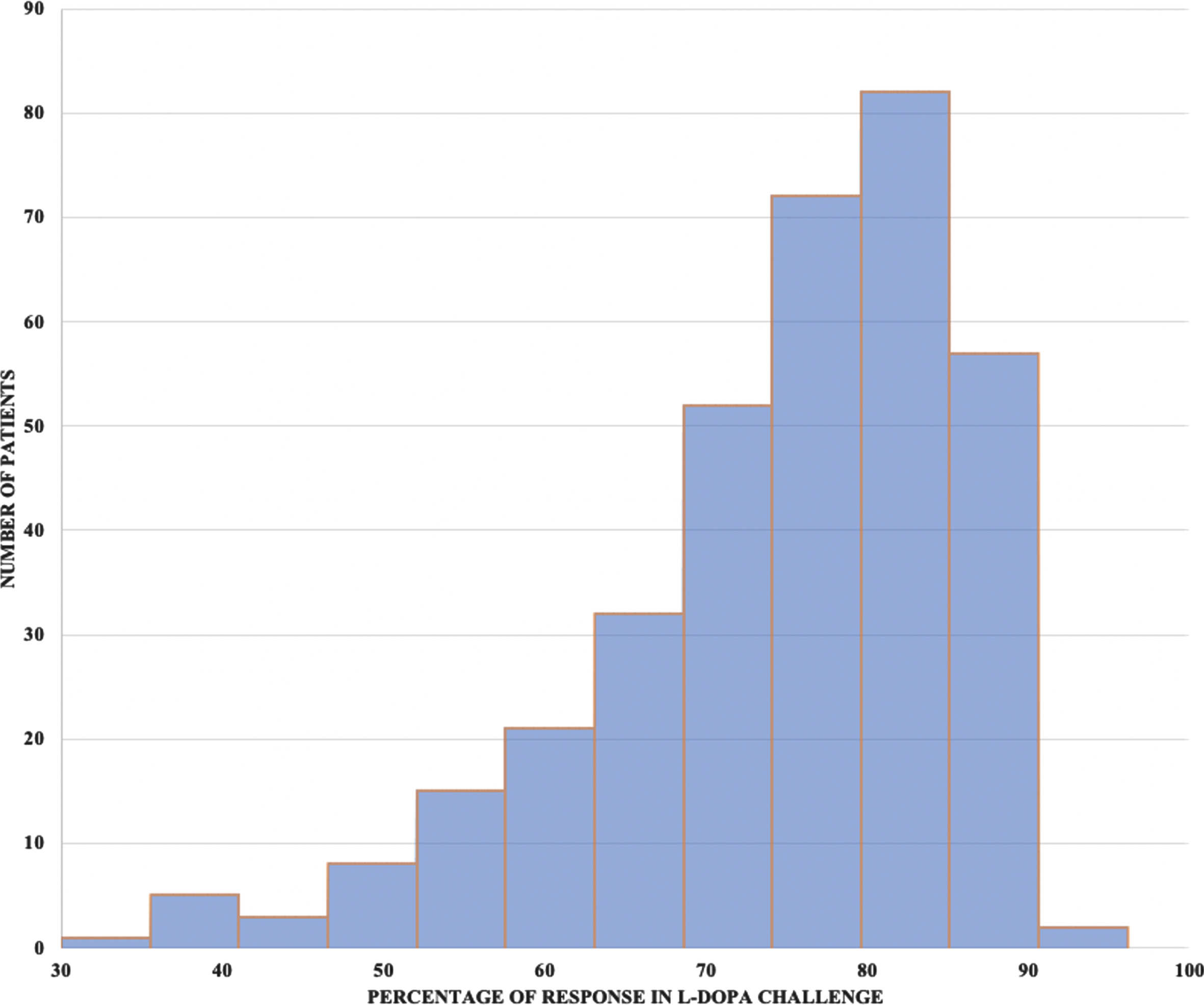
Frequency distribution of L-dopa response in the study population.

Imaging and features

All patients were scanned on 3T MRI systems. Two sequences were obtained: (i) high-resolution 3-dimensional T1w; and (ii) multi-gradient echo (Multi-GRE) T2*w sequences. Both sagittal sequences had 1 mm³ isotropic voxels; for the T1w sequence, parameters were: repetition time = 7.2 ms, echo time = 3.3 ms, flip angle = 9°, acquisition matrix = 256×256, and 176 contiguous slices, while for the multi-GRE T2*w sequence, they were TR = 54 ms, TE = 4.2, 9.5, 14.7, 20, 25.3, 30.5 ms, flip angle = 15°, acquisition matrix = 256×256, and 160 contiguous slices.

Imaging features were extracted from the key cerebral structures affected in PD. In addition to the substantia nigra, the caudate nucleus and the putamen the primary sites of the disease, the sub-thalamic nucleus, the target of DBS and the thalamus were also considered as regions of interest (ROI) because they are impacted by cell loss [12–15].

Structural T1 images were processed using the HCP pipeline (workbench 1.4.2) [16]. This optimized pre-processing pipeline includes steps for non-uniform signal correction, signal and spatial normalizations, skull stripping, and brain tissue segmentation based on Freesurfer software [17]. The caudate, putamen, and thalamus were segmented using the Volbrain pipeline [18]. The substantia nigra and sub-thalamic nucleus were segmented using the atlas described by Keuken et al. [19]

R2* mapping was performed with niftyfit [20]. A mono-exponential isotropic decay with echo time was obtained by voxel-by-voxel nonlinear least-squares fitting of the multi-echo T2*-weighted data.

For features computing, we considered texture analysis to measure different statistics quantifying signal variation in the defined brain regions. This technique has been proven to be effective at detecting changes related to the disease on different MRI sequences: T1 [21], [22], R2*, and QSM maps [23]. According to our experience with these features, 10 texture features were chosen and computed: four from first-order statistics and six from second-order statistics. The first-order parameters included: mean gray level, standard deviation (SD) of gray levels, kurtosis, and skewness. These two last features allow quantification of the asymmetry of signal values in relation to a normal distribution.

The second-order features (also known as Haralick textural features) quantify the relationships between pairs of neighboring voxels in the image. The features were derived from the gray level co-occurrence matrix (GLCM); a spatial relationship was defined as the relative direction in a given direction d. In this study, the GLCM matrix was estimated by considering four directions (θ= 0°, 45°, 90°, and 135°) and a distance d = 1 voxel. Using this matrix, the following features were computed: homogeneity, which represents uniformity of the texture intensity; contrast, which represents the degree to which the texture intensity levels differ between voxels or local intensity variation; entropy, which represents the degree of uncertainty (measure of randomness); correlation, which represents the degree of mutual dependency between voxels; variance, which gives high weights for elements different from the average value; sum-average, which measures the relationship between occurrences of pairs with lower intensity values and occurrences of pairs with higher intensity values; and inverse difference moment (InvDiff), which measures the difference between the highest and lowest values of a contiguous set of voxels.

Texture features were measured in the five regions indicated above in T1w images while on the R2* maps, they were computed in the substantia nigra and sub-thalamic nucleus (Fig. 2).

Fig. 2

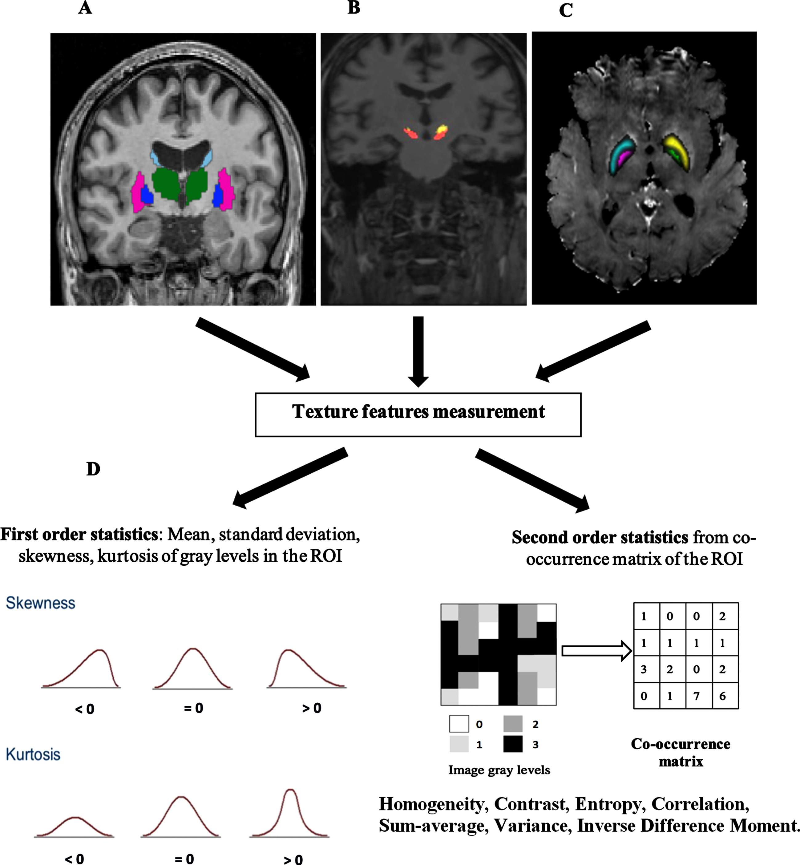
Images and features. A) MRI T1-weighted image. B) Definition of the structures of interest, caudate nucleus, putamen, and thalamus on T1 images. C) Definition of the substantia nigra and sub-thalamic nucleus on T1 images. C) Right R2* maps with regions of interest (ROI) on the substantia nigra and sub-thalamic nucleus. D) Texture features computing process.

Modeling

Accurate model building requires three steps. The first involves the definition of features to be considered, the second involves combination of these features to obtain the best estimation of the outcome (i.e., here the percentage L-dopa response), and the third is testing and validating the model. For the first step, different configurations were considered by enhancing the complexity of the features studied. The first model (Demo_Clinic_Model) looked at demographic and clinical data measured during “ON” conditions (Table 1). The other models incorporated imaging features in the first model. The second focused on features from T1w images (Demo_Clinic_T1_Model) and the third focused on features from R2* maps (Demo_Clinic_R2*_Model), while the last considered the combination of T1w and R2* features (Demo_Clinic_T1_R2*_Model).

For the second step, given that the variable to be estimated is quantitative and continuous, regression-based approaches are the most suitable among the machine learning methods. From another side and by considering the incremental complexity that we want to test in the models and lastly guided by the aim of obtaining a clinically meaningful models allowing to assess the contribution of each contributor variable and its weighted, we have selected the Least Absolute Shrinkage and Selection Operator (LASSO) algorithm [24] (In MATLAB, MathWorks Inc., Natick, MA, USA). This is a multivariate regression analysis method, based on shrinkage estimation. It has different advantages, including overall variable selection, a capacity to handle multi-collinearity, and a reduction of the possibility of model over-fitting. Interestingly, the LASSO enables the first and second steps to be combined.

The testing and validation step consisted of an estimation of the performance of the model. It included cross-validation, using the data used for learning, and testing using new and unseen data. To deal with this step, and given the dataset size, we chose to use a sub-part of the data for model building and a second sub-part for testing. In order to make the testing data completely unseen for the learning process, data from some centers were not included in the learning process and were exclusively used for testing purpose as external data. Thus, the 13 movement disorder centers involved in the study were randomly divided into learning and testing sets with the aim of having 80% of the data for learning and 20% for testing, commonly used in machine learning methods. Random selection was therefore applied to select the centers to obtain data from 280 patients for learning. These 280 patients were recruited in 10 centers. Data from the remaining three centers with 70 patients were used for testing. This process is summarized in Fig. 3. The distributions of the main demographic and clinical scores in the learning and testing sets are described in Table 2.

Fig. 3

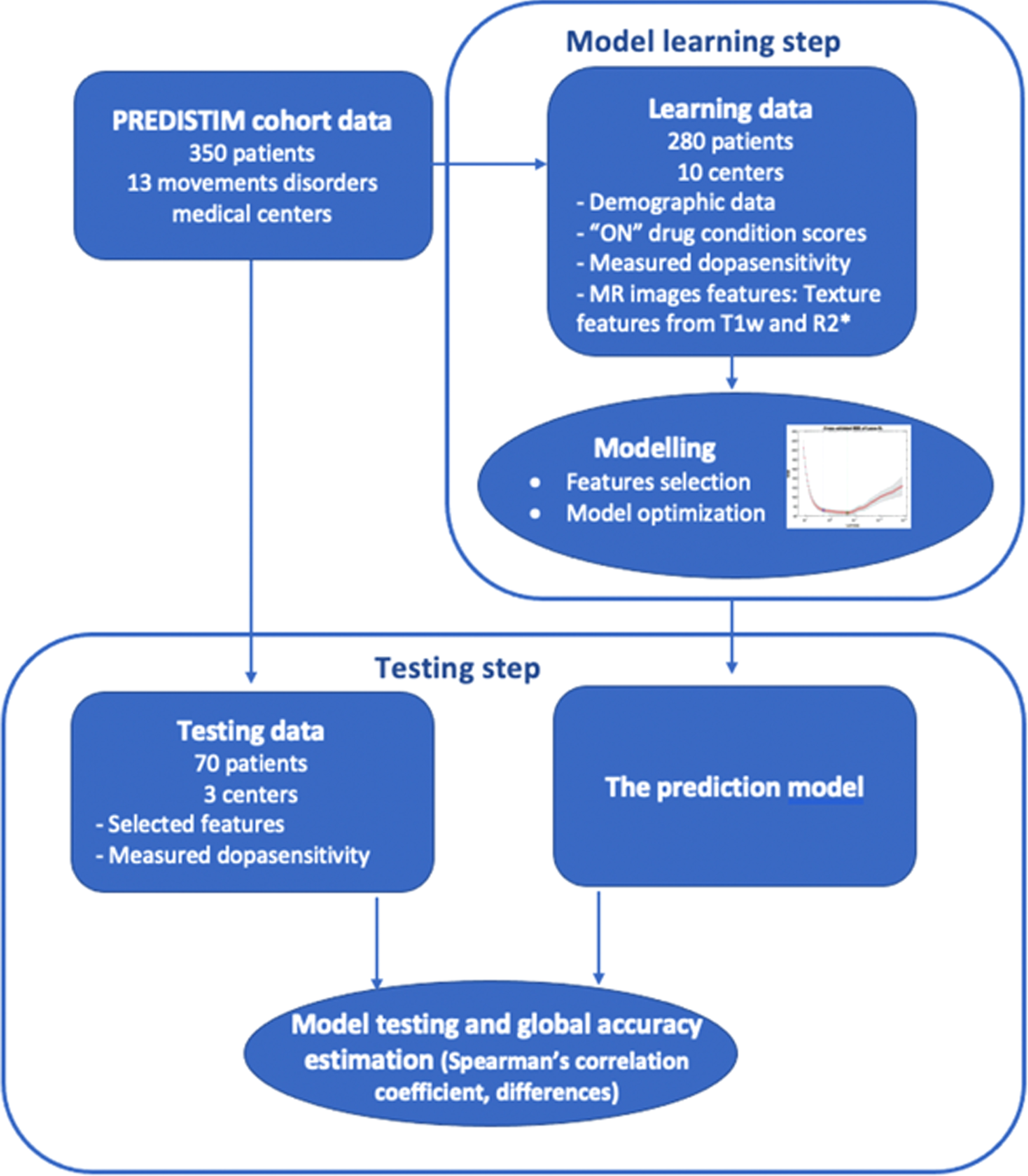
Flowchart of the process for building the dopa-sensitivity prediction model with the two steps: model estimation and model testing.

Table 2

Data distribution in the learning and testing sets

	Learning data	Testing data
No. of patients	280	70
No. of centers	10	3
Sex (M/F)	190/90	45/25
Age (y)	60.1±8.2	58.7±7.8
Disease duration (y)	10.3±4.2	9.2±3.85
LEDD (mg/day)	1700.32±350.190	1690.75±400.85
Dopa-sensitivity (%)	72.05±10.5	74.50±9.75

Values shown are mean±standard deviation unless stated otherwise. M, male; F, female; LEDD, L-dopa equivalent dose.

From another side and given that data distribution is unbalanced (Fig. 1) and most of the included patients (260) exhibited a dopa-sensitivity > 70% and the remaining (90) were in the range 30–70%, which may impact the quality of the modelling, we aimed to test the performances of the models separately on the range > 70% which appears, in terms of size, the most suitable for data analysis and modelling.

Performances evaluation

Performances in the learning and testing datasets were measured by comparing the actual dopa-sensitivity values and the estimated values using the coefficient of determination (R²), min, max and the mean absolute differences [25].

RESULTS

The overall results for the four models built are summarized in Table 3.

Table 3

Performances of the four prediction models built to estimate dopa-sensitivity using the learning and testing datasets

Model	Learning				Testing
	Mean	Min	Max	R2 *	Mean	Min	Max	R2 *
Demo_Clinic_Model	5.9	–20	22	0.69	6.25	–25	18	0.60
Demo_Clinic _T1_Model	5.1	–20	20	0.76	6	–20	18	0.65
Demo_Clinic_R2_Model	5.7	–23	20	0.72	7	–20	15	0.60
Demo_Clinic_T1_R2_Model	5	–20	19	0.76	8	–23	19	0.55

*p < 0.0001. R², Coefficient of determination. Min, Minimum difference between actual and estimated dopa-sensitivity values. Max, Maximum difference between actual and estimated dopa-sensitivity values. Mean, Mean absolute difference between actual and estimated dopa-sensitivity values.

The first model the Demo_Clinic_Model, the simplest since it includes only demographic and clinical scores on “ON” condition was built using the following features: age, sex, disease duration, MDS_UPDRS 2 (ON), MDS_UPDRS 3 (ON), MDS_UPDRS 4, and Schwab_England (ON). The full regression equation was: $\begin{array}{cc}\hfill & \text{Dopasensitivity}\_\text{Demo}\_\text{Clinic}\_\text{Model}\hfill \\ \hfill & =-0.035*\text{age}+0.191*\text{disease}\_\text{duration}\hfill \\ \hfill & +0.041*\text{gender}+0.341*\text{MDS}\_\text{UPDRS}2\hfill \end{array}$ $\begin{array}{cc}\hfill & -1.594*\text{MDS}\_\text{UPDRS}3\hfill \\ \hfill & +0.494*\text{MDS}\_\text{UPDRS}4\hfill \\ \hfill & +0.11*\text{Shwab}\_\text{England}+76.310\hfill \end{array}$

After optimization on the learning data, the model showed a coefficient of determination of R² = 0.60 (Pearson correlation coefficient r = 0.77, p < 0.001) on the unseen data, while the performances were R² = 0.69 (Pearson correlation coefficient r = 0.83, p < 0.001) on the learning set. When the performances were assessed using data from the range (dopa-sensitivity > 70%), the performances grew to R² = 0.80 in the testing set and R² = 0.85 in the learning set. The deviation between the actual values and the estimated one were in the range [min = –10, max = +5]. Figure 4A depicts the behavior of this model on the learning and testing datasets.

Fig. 4

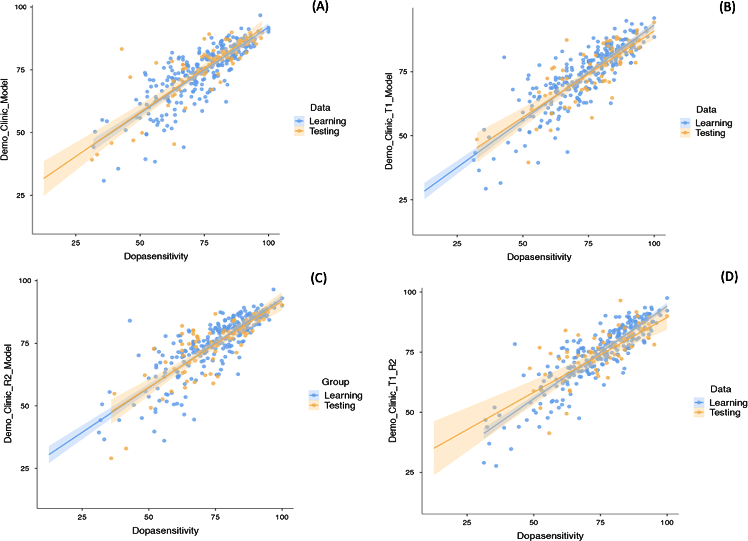
Actual and estimated dopa-sensitivity values in the prediction models on the cross-validation and testing sets, and their respective 95% confidence intervals. A) Model with demographic and clinical data. B) Model with demographic and clinical data, and texture features from T1w images. C) Model with demographic and clinical data, and texture features from R2* maps. D) Model with demographic and clinical data, and texture features from T1w images and R2* maps.

The Demo_Clinic_T1_Model enhanced the performances of the first model (R² = 0.65, Pearson correlation coefficient r = 0.80, p < 0.001) in the testing set (R² = 0.76, Pearson correlation coefficient r = 0.87, p < 0.001 in the learning set). A slight enhancement was also observed for the data in the range (dopa-sensitivity > 70%): R² = 0.82 in the testing set and R² = 0.88 in the learning set respectively. Deviation between the actual and estimated values was in the range [min = –7, max = +5]. (Fig. 4B). For this model, the selection step retained the same clinical and demographic features as previously in addition to the following T1w imaging features: entropy from the substantia nigra (SN), energy and entropy from the thalamus, InvDiff from the putamen, and skewness from the caudate. The full regression equation was as: $\begin{array}{cc}\hfill & \text{Dopasensitivity}\_\text{Demo}\_\text{Clinic}\_\text{T}1\_\text{Model}\hfill \\ \hfill & =-0.04*\text{age}+0.22*\text{disease}\_\text{duration}\hfill \\ \hfill & +0.05*\text{gender}+0.25*\text{MDS}\_\text{UPDRS}2\hfill \end{array}$ $\begin{array}{cc}\hfill & -1.60*{\text{MDS}}_{\text{UPDRS}3}+0.55*{\text{MDS}}_{\text{UPDRS}4}\hfill \\ \hfill & +0.15*\text{Shwab}\_\text{England}-0.4*{\text{Entropy}}_{\text{SN}}\hfill \\ \hfill & +0.66*{\text{Energy}}_{\text{Thalamus}}-0.57*\hfill \\ \hfill & {\text{Entropy}}_{\text{Thalamus}}+0.03*{\text{InvDiff}}_{\text{Putamen}}\hfill \\ \hfill & +0,05*{\text{Skewness}}_{\text{Caudate}}+72.05\hfill \end{array}$

The Demo_Clinic_R2*_Model that considered the features from the R2* maps was built using the regression equation: $\begin{array}{cc}\hfill & \text{Dopasensitivity}\_\text{Demo}\_\text{Clinic}\_\text{R}2\_\text{Model}\hfill \\ \hfill & =-0.08*\text{age}+0.35*\text{disease}\_\text{duration}\hfill \\ \hfill & +0.1*\text{gender}+0.30*\text{MDS}\_\text{UPDRS}2\hfill \end{array}$ $\begin{array}{cc}\hfill & -1.85*{\text{MDS}}_{\text{UPDRS}3}+0.88*{\text{MDS}}_{\text{UPDRS}4}\hfill \\ \hfill & +0.15*\text{Shwab}\_\text{England}-0.7*{\text{Entropy}}_{\text{SN}}\hfill \\ \hfill & +0.08*{\text{Kurtosis}}_{\text{SN}}-0.3*{\text{Entropy}}_{\text{STN}}\hfill \\ \hfill & +74.65\hfill \end{array}$

It can be observed that this model included the same clinical and demographic features as those used in the first model and added entropy and kurtosis from the substantia-nigra as well as the entropy from the sub-thalamic nucleus. The model showed very close performances as the Demo_Clinic_Model (R² = 0.60 and 0.72 in the testing and learning datasets respectively). But when considering only the range (dopa-sensitivity > 70%), it outperforms this first model R² = 0.85 in the testing set and R² = 0.90 in the learning set respectively with a deviation between the actual and estimated values < ±5 units (Fig. 4C).

For the last model all the features were considered for the selection, the LASSO algorithm selected the same clinical and demographic features as in the first model and completed by MR imaging features: entropy from the substantia nigra, InvDiff from the putamen and skewness from the caudate from the T1w images and kurtosis from the SN from the R2* maps. The equation of the model was:

$\begin{array}{cc}\hfill & \text{Dopasensitivity}\_\text{Demo}\_\text{Clinic}\_\text{T}1\_\text{R}2\_\text{Model}\hfill \\ \hfill & =-0.05*\text{age}+0.41*\text{disease}\_\text{duration}\hfill \\ \hfill & +0.01*\text{gender}+0.30*\text{MDS}\_\text{UPDRS}2\hfill \end{array}$ $\begin{array}{cc}\hfill & -1.82*{\text{MDS}}_{\text{UPDRS}3}+0.80*{\text{MDS}}_{\text{UPDRS}4}\hfill \\ \hfill & +0.23*\text{Shwab}\_\text{England}-0.52*{\text{Entropy}}_{\text{SN}\_\text{T}1}\hfill \\ \hfill & -0.07*{\text{InvDiff}}_{\text{Putamen}\_\text{T}1}+0.23*{\text{Skewness}}_{\text{Caudate}\_\text{T}1}\hfill \\ \hfill & +0.1*{\text{Kurtosis}}_{\text{SN}\_\text{R}2}+72.05\hfill \end{array}$

In this model, the performances in the testing dataset felt down (R² = 0.55, Pearson correlation coefficient r = 0.74, p < 0.001) and also in the range (dopa-sensitivity > 70%), R² = 0.78 in the testing set and R² = 0.83 in the learning set.

DISCUSSION

Prediction of clinical scores for patients with PD is clinically relevant but remains challenging, requires the use of massive amounts of data [26] and accurate learning methods to link the observations to the inputs [27]. This study focused on the estimation of patient individual dopa-sensitivity. The phenotypic heterogeneity of PD includes variability in L-dopa responsiveness [1, 28–30]. The underlying mechanisms as well as the clinical correlates and significance of this heterogeneity are not clearly defined. The study exploits data from a large clinical trial to evaluate different configurations of prediction models. Patients were recruited for DBS and underwent L-dopa challenge to estimate their dopa-sensitivity. The modelling strategy was based on two factors: (i) the use of a small set of variables, clinically meaningful; and (ii) maximization of accuracy. Hence, to define the optimal variables to be incorporated, they were winnowed down through machine learning in different conditions. The first model considered only of demographic and clinical scores measured in “ON” conditions, once the patients received their daily L-dopa dose. The other models incorporated variables from MRI with sequences that demonstrated their usefulness in PD. Consequently, the second model included features from T1w images, the third from R2* maps, and the fourth from both sequences. The global performances of the four models are summarized in Table 3.

The modelling process included a discovery part involving 80% of the population from 10 randomly selected centers and a validation step involving the remaining 20% of patients from three centers. Ideally, the validation cohort would be external to the study; however, even though dopa-sensitivity was always measured as the difference between “ON” and “OFF” scores, and according to a defined protocol (see Methods), the methods used to evaluate sensitivity to an acute L-dopa challenge could have varied slightly between centers and evaluators and the data used can therefore be considered as representative of the procedure.

Additionally, and by considering the unbalanced distribution of the data, it seemed appropriate to assess the models in a specific configuration where data size was more suitable for data modelling. This was the case for the range (dopa-sensitivity > 70%). The global performances were better than when using all the available data, in both learning and testing sets. Interestingly, for these data, a decrease was observed in the margin errors between the actual dopa-sensitivity values and the estimated ones.

The first model Demo_Clinic_Model, the simplest one, was built by combing in the regression model, the patient’s age, sex, and disease duration, as well as scores measuring motor complications: MDS_UPDRS 2 score, which quantifies motor experiences of daily living, MDS_UPDRS 3 score for motor examination, MDS_UPDRS 4 for motor complications, and the Schwab & England score for activities of daily living. For this model, the coefficient of determination R² was 0.69 and 0.60 for the learning and test sets, respectively (Fig. 3A). For the range (dopa-sensitivity > 70%), the R² grows in the testing set to 0.80 and a range error of [–10, +5]. Malek et al. [28] in the Tracking Parkinson’s study, which investigated L-dopa responsiveness in early PD, examined demographic and disease-related features and found that older patients had a less robust response to L-dopa, and identified a relationship between dopa-sensitivity and motor scores. In the study by Hauser et al. [2], sex influence was highlighted with female gender showing lower responses. In the same way, it was reported that L-dopa responsiveness could be influenced by a patient’s pharmacokinetics. Warren et al. [31] described the potential contribution of body weight while Mukherjee et al. [32] reported the impact of gut absorption. The features selected to build the Demo_Clinic model seem to reflect all these variability sources and consequently their combination allowed us to obtain an accurate estimation of dopa-sensitivity.

In subsequent models, we aimed to take advantage of neuroimaging, mainly MRI, to enhance the modeling accuracy. In addition to the fact that MRI in PD was reported to be of interest for disease diagnosis and staging, with correlation between some imaging features and some clinical scores, L-dopa is associated with changes in the images [8, 33]. L-dopa administration induces intensity variations. Probably, influenced by the presence of iron, T2 relaxation time was reported to be shorter [34, 35]. On T1w sequences, voxel-based morphometry demonstrated an increase in gray matter voxel number in the substantia nigra, tegmental ventral area, and sub-thalamic nucleus [36]. For these models, it can be observed that the demographic and clinical features used for the first model were also selected as predictors. Only their weighting differed between the models. As discussed above, this may be explained by the fact that these features are the main contributors for the dopa-sensitivity variations explanation.

In that way, the second model (Demo_Clinic_T1_Model) investigated the contribution of the imaging features measured on T1w images. Among the potential features that can be used, we chose to use texture features measured in ROI from the nigrostriatal pathway. These features have been demonstrated to have greater sensitivity to detect intensity changes than volumetry and morphometry analysis methods [22]. Consequently, the model adding these features to the demographic and clinical features enhanced the performance to R² of 0.76 in the learning set and 0.65 in the validation set, respectively (Fig. 3B). In the range (dopa-sensitivity > 70%), the R² grows in the testing set to 0.82 and a range error of [–7, +5].

The contribution of features extracted from the R2* maps was examined in the model Demo_Clinic_R2_Model which additionally to the clinical and demographic predictors, selected imaging features from the substantia nigra and the sub-thalamic nucleus. One of the aspects of PD is abnormal iron accumulation in different regions of the brain, mainly the substantia nigra and sub-thalamic nucleus. This model, when considering all the data, did not outperform the two previous, however, when assessed using data in the range (dopa-sensitivity > 70%), enhanced the coefficient of determination to 0.85 in the testing set with a estimation error < ±5 units (Fig. 4C).

The last model combined clinical and demographic data with images features from both modalities but as it can observed in Fig. 4D this combination did not allow to the enhancement of the prediction performances.

This study is a proof of concept towards the computational modelling of dopamine responsiveness. The outcomes, that should be validated in larger patients population, including dopa-resistant patients (dopa-sensitivity < 30%), indicate that it could be feasible to have an estimation of patient’s individual dopa-sensitivity without an acute dopa challenge to put the patients in “OFF” conditions. Without claiming to completely replace the L-dopa challenge, which remains the standard, and beyond the quantitative aspect of dopa-sensitivity measurement, it allows the clinician to appreciate the qualitative aspects of L-dopa effects, the proposed approach described here may have a clinical impact on the selection of patients for DBS by allowing a preliminary overall estimation of the responsiveness. To the best of our knowledge, this is the first study to deal with this issue in this manner: using only “ON” scores and by considering the output variable as it is, i.e., a continuous variable. In the two first attempts, patients were stratified. In Aman et al. [6], the 28 patients included in the study were organized into two groups: good responders and bad responders and the problem was solved as a binary classification problem. In the study by Khodakarami et al. [5], in addition to the fact that the method is based on the use of a medical device, the 199 patients of the study were stratified into 5 classes according to the score on the UPDRS 3.

The outcome of the study should be considered carefully and seen as a first step towards the use of analytical modelling for dopa-sensitivity estimation. Indeed, it tells that mathematical modelling and machine learning can help in building clinically applicable solutions. The following steps could be at two levels. The first, the use of larger datasets from general PD patients, not only those recruited for DBS. Indeed, as showed when the models were assessed using data in the range (dopa-sensitivity > 70%) the performances were higher and become potentially clinically applicable with estimation errors < ±5 units. Furthermore, the availability of more massive and representative data of the PD patients will allow the use of additional modelling algorithms. Deep learning methods as conventional neural network would likely being suitable to extract potential features from the T1 and R2* maps [37]. The second is the definition of acceptable margins errors for the estimated values according to the considered clinical application.