Sage Journals: Discover world-class research

Abstract

Remanufacturing, with its environmental and economic implications, is gaining significant traction in the contemporary industry. Owing to the complementarity between remanufacturing process planning and scheduling in actual remanufacturing systems, the integrated remanufacturing process planning and scheduling (IRPPS) model provides researchers and practitioners with a favorable direction to improve the performance of remanufacturing systems. However, a comprehensive exploration of the IRPPS model under uncertainties has remained scant, largely attributable to the high complexity stemming from the intrinsic uncertainties of the remanufacturing environment. To address the above challenge, this study proposes a new IRPPS model that operates under such uncertainties. Specifically, the proposed model utilizes interval numbers to represent the uncertainty of processing time and develops a process planning approach that integrates various failure modes to effectively address the uncertain quality of defective parts during the remanufacturing process. To facilitate the resolution of the proposed model, this study proposes an extended non-dominated sorting genetic algorithm-II with a new multi-dimensional representation scheme, in which, a new self-adaptive strategy, multiple genetic operators, and a new local search strategy are integrated to improve the algorithmic performance. The simulation experiments results demonstrate the superiority of the proposed algorithm over three other baseline multi-objective evolutionary algorithms.

Keywords

Integrated remanufacturing process planning and scheduling remanufacturing systems uncertainty environment interval processing time non-dominated sorting genetic algorithm-II

1 Introduction

The contradiction between the rapid development of society and environmental pollution has become increasingly prominent. As an important part of sustainable development, remanufacturing of end-of-life (EOL) products has attracted increasing attention in recent years [1, 2]. In remanufacturing systems, EOL products are restored to like-new condition by means of complete disassembly, reprocessing of defective parts, and reassembling [3]. Because traditional decision-making approaches are not effective in dealing with the complexity of EOL products in uncertain remanufacturing systems, different levels of remanufacturing decision-making approaches have been proposed at the strategic level [4], tactical level [5], and operational level [6].

Remanufacturing process planning and scheduling are two critical issues at the operational level in actual remanufacturing systems [1, 7]. Remanufacturing process planning provides guidance for the global scheduling of workshops according to resource constraints. Shop scheduling obtains the operation sequence of the machines within a specified time according to the process plan constraints. These two critical issues are dealt with separately and sequentially in traditional remanufacturing systems [8, 9]. However, this hinders the improvement of remanufacturing productivity and performance, and may lead to conflicts between the objectives of remanufacturing process planning and scheduling [10], e.g., the pre-defined process plans may be infeasible during the scheduling phase.

To overcome this problem, the current study focuses on the integration of remanufacturing process planning and scheduling. Compared with the traditional manufacturing environment, remanufacturing systems have more intrinsic uncertainties, such as highly variable processing times, uncertain quality of defective parts, and stochastic routings for reprocessing operations [3]. A few studies have investigated the integrated remanufacturing process planning and scheduling (IRPPS) models in remanufacturing system, however, they ignored either the uncertain quality of defective parts or the uncertainty of processing time. In practice, the processing time of an EOL product in a remanufacturing system is not always fixed and may fluctuate within an interval because of its intrinsic uncertainty. In addition, the selection of a process plan based on the quality differences of defective parts is more conducive to the improvement of remanufacturing scheduling efficiency and the reduction of energy consumption. Therefore, establishing a mathematical model under uncertainties is more suitable for an actual remanufacturing environment.

To fill the above gaps, a new IRPPS model is proposed to coordinate the process planning and scheduling under uncertainties in remanufacturing systems with the objective of minimizing energy consumption, makespan, and maximum machine load, which considers not only the uncertainty of processing time, but also the uncertainties related to the quality of defective parts. The proposed model utilizes interval numbers to represent the uncertainty of processing time and develops a process planning approach that integrates various failure modes to effectively address the uncertainties during the remanufacturing process.

The IRPPS problem is a typical multi-objective NP-hard problem. Up to now, researchers have investigated Pareto-based multi-objective evolutionary algorithms to tackle a variety of NP-hard problems. In recent years, the non-dominated sorting genetic algorithm-II (NSGA-II) [11] has been extensively implemented and has achieved good performance [12 –14] to tackle various multi-objective optimization problems. However, the basic NSGA-II cannot be directly applied to address the IRPPS model because its standard one-dimensional representation scheme does not model the multiple dimensions of the IRPPS model comprehensively. In addition, the basic NSGA-II has several weaknesses, including weak exploitation and exploration abilities. Therefore, an extended NSGA-II (ENSGA-II) is proposed in this study for solving the IRPPS model. The proposed ENSGA-II has extended the basic NSGA-II by incorporating a new multi-dimensional representation scheme, a new self-adaptive strategy, and a new local search strategy. Simulation experiments are performed through different instances, demonstrating that the ENSGA-II is superior to the three other baseline multi-objective algorithms.

The contributions of this paper are the following:

A new IRPPS model with the objective of minimizing energy consumption, makespan, and maximum machine load is proposed for the first time and a mathematical model is established.

The proposed model comprehensively considers the uncertainties of the remanufacturing environment. It utilizes interval numbers to represent the uncertainty of processing time and develops a process planning approach that integrates various failure modes.

In order to solve the proposed model, an ENSGA-II with a new multi-dimensional scheme is proposed, integrating a new self-adaptive strategy and multiple genetic operators to enhance population diversity, and designing a new local search strategy to improve the algorithmic efficiency.

Experiments are conducted on 24 sets of instances, which shows that the proposed algorithm outperforms the three other baseline multi-objective algorithms in solving the proposed model, and highlights its efficacy and potential for broader applications in the realm of remanufacturing systems.

This paper is organized as follows. Section 2 outlines the cutting-edge technologies. Section 3 presents a new IRPPS model under uncertainties. Section 4 provides the introduction of the basic NSGA-II and proposes the ENSGA-II for solving the IRPPS model. Section 5 provides the experiments conducted to evaluate and compare the performance of the ENSGA-II. Section 6 concludes this study and presents future work.

2 Related work

Remanufacturing process planning and scheduling have received much attention as two critical issues in actual remanufacturing systems. This section demonstrates the cutting-edge technologies from three aspects and summarizes the gaps to be filled.

2.1 Remanufacturing process planning and scheduling

Most of the existing studies on remanufacturing systems focus on remanufacturing process planning or scheduling of remanufacturing shops. For example, Wang et al. [8] proposed a fault feature characterization-based optimization method to solve the remanufacturing process planning problem. Shi et al. [6] presented an environmentally friendly remanufacturing scheduling system that involves parallel flow-shop-type non-dedicated reprocessing lines. Zhang et al. [9] constructed a multi-objective scheduling model that integrated parallel disassembly/reassembly shops and a flexible job-shop-type reprocessing shop with the aim of reducing makespan and energy consumption. Zhang et al. [15] developed an uncertain remanufacturing scheduling model that takes into account the risk of rework during the remanufacturing process. Wang et al. [16] studied the energy-aware remanufacturing system scheduling model by integrating three core production stages, i.e., disassembly, reprocessing, and reassembly. Guo et al. [17] proposed an integrated scheduling method for a disassembly-reprocessing-reassembly remanufacturing system that considers the commonality of components, aiming to minimize both makespan and energy consumption.

However, the above studies only addressed remanufacturing process planning and scheduling separately, and research on IRPPS modeling is still in its infancy. Owing to the high complexity of remanufacturing systems, the scheduling factors should be considered during remanufacturing process planning to address the conflicts between the objectives of remanufacturing process planning and scheduling. Hence, Zhang et al. [18] studied the IRPPS model with two probably conflicting objective functions, considered both remanufacturing process planning and scheduling, and addressed this model using simulation-based optimization. Gong et al. [1] presented an evolutionary IRPPS model with five optimization objectives and tackled it using a hybrid multi-objective evolutionary algorithm. Zhang et al. [19] proposed an IRPPS model that incorporates parallel disassembly workstations, a flexible job-shop-type reprocessing shop, and parallel reassembly workstations. Zhang et al. [20] proposed an energy-efficient multi-objective IRPPS model that focuses on the energy efficiency in the IRPPS model.

However, the existing IRPPS models have not comprehensively addressed the intrinsic uncertainties of remanufacturing systems. They ignored either the uncertainty of the processing time of defective parts, or the uncertainties related to the quality of defective parts and their production. In addition, these studies did not properly consider the integration of resource constraints to realize energy-efficient remanufacturing. Thus, this study proposes a new IRPPS model to fill these gaps. A feasible modeling scheme is given to coordinate the process planning and scheduling more comprehensively under remanufacturing uncertainties.

2.2 Interval number theory

In many previous studies, uncertainty-based mathematical analysis theories (e.g., rough set theory, fuzzy theory, grey system theory, etc.) have been used to describe the uncertainties of the remanufacturing environment [21]. However, these methods have disadvantages in that they rely on known membership and probability distribution functions before formalizing an uncertainty model. The integration of interval number theory with uncertainty modeling can overcome these difficulties.

In recent years, the interval number theory has been widely applied to optimization areas [22]. In particular, shop scheduling problems constructed with interval numbers have received extensive attention from researchers. For instance, Jamrus et al. [23] constructed the flexible job-shop scheduling problem (FJSSP) for semiconductor fabrication, in which the processing times are represented as intervals. Fang et al. [24] defined the processing time as the interval numbers in a disassembly shop to construct an appropriate uncertainty model.

The above studies have mainly elaborated on shop scheduling problems using interval number theory. However, few studies have focused on the IRPPS model combined with the interval number theory. Hence, the current study attempts to solve the IRPPS model using the interval number theory under the uncertainties of remanufacturing systems.

The basic interval arithmetic of the interval numbers is shown in Equations (1)–(3) [22]. For example, let A = [A_L, A_R] (or A = {A_C, A_W}) and B = [B_L, B_R] (or B = {B_C, B_W}) be two interval numbers. $A \oplus B = [A_{L} + B_{L}, A_{R} + B_{R}]$ (1) $A ⊖ B = [A_{L} - B_{L}, A_{R} - B_{R}]$ (2) $λ \cdot A {\begin{matrix} λ [A_{L}, A_{R}] for λ \geq 0 \\ λ [A_{R}, A_{L}] for λ \leq 0 \end{matrix}$ (3) where A_L and A_R represent the lower and upper bounds of interval number A, respectively. λ is scalar. If A_L = A_R, A is a real number. A_C and A_W represent the mid-point and half-width of interval number A, respectively, where A_C = (A_L + A_R)/2 and A_W = (A_R–A_L)/2.

The interval order relations between two intervals A and B for the minimization problems are shown in Equation (4) [25]. $\begin{matrix} A \leq^{min} B \Leftrightarrow {\begin{matrix} A_{C} < B_{C} if A_{C} \neq B_{C} \\ A_{W} \leq B_{W} if A_{C} = B_{C} \end{matrix} \\ and A <^{min} B \Leftrightarrow A \leq^{min} B and A \neq B \end{matrix}$ (4) where < ^min and ≤^min represent the order relation between two intervals.

2.3 Multi-objective optimization algorithms

Recently, multi-objective optimization algorithms have been widely used in process planning and scheduling fields. For example, Huang et al. [26] proposed and demonstrated that an improved multi-objective particle swarm optimization (MOPSO) algorithm could efficiently address the FJSSP. Fang et al. [24] presented a disassembly scheduling problem with different capability constraints imposed on the robots and solved it using a multi-objective simulated annealing algorithm. Abed-Alguni and Alawad [27] proposed a discrete variation of the Distributed Grey Wolf Optimizer to handle dependency task problems on virtual machines with the objective of minimizing computation and data transmission costs. Wang et al. [28] presented a multi-objective optimization algorithm, which incorporates a multi-region division sampling strategy, a genetic algorithm and a differential evolutionary algorithm for solving the flexible job shop scheduling problem. Alawad and Abed-alguni [29] proposed a discrete island-based cuckoo search algorithm with a highly disruptive polynomial mutation and an opposition-based learning strategy for scheduling workflow applications in cloud computing environments. Bezdan et al. [30] applied the Pareto-based hybrid bat algorithm to deal with the cloud computing task scheduling problem. Lu et al. [31] utilized a Pareto-based collaborative multi-objective optimization algorithm to tackle an energy-efficient flow shop scheduling problem. Liu et al. [32] applied a hybrid meta-heuristic algorithm to solve the problem of appliance scheduling, with the goal of minimizing electricity costs and user dissatisfaction.

In particular, the NSGA-II has been widely adopted to solve multi-objective scheduling problems owing to its good performance in engineering optimization. For example, Wu and Sun [33] employed NSGA-II to address the FJSSP, which involves the energy-saving factors. Zhang et al. [34] presented a game-theoretic-based NSGA-II to schedule business services provided by different manufacturers. Yuan et al. [35] improved the NSGA-II by incorporating several enhancements including a modified evaluation function, a competition mechanism, a cross-variance strategy, and an elite retention strategy to solve the workshop resource scheduling problem. Afsar et al. [36] proposed a multi-objective enhanced memetic algorithm that combines NSGA-II with three intensification strategies to solve the green job shop scheduling problem. It is worth noting that, according to the design principles of memetic algorithms [37], the ENSGA-II proposed in this study can also be considered as a memetic algorithm. Wang et al. [38] implemented an extended NSGA-II specifically tailored for the hybrid flow shop scheduling problem with variable machine speeds. Deng et al. [14] integrated the NSGA-II, fuzzy rough set, and sliding window to forecast and simulate the high-frequency price directions of crude oil futures in the market.

In this study, the NSGA-II is employed to address the proposed IRPPS model. However, the basic NSGA-II only uses a one-dimensional representation scheme, which cannot be directly used to solve the proposed IRPPS model with multiple dimensions. In addition, the exploitation and exploration abilities of the basic NSGA-II still have room for improvement. Therefore, a new ENSGA-II is proposed in this study to solve the IRPPS model.

Table 1
An illustration of the flexible process plans

Feature Failure mode Candidate operations Candidate machines Processing time Feature constraints

F ₁ FM ₁₁ O ₁ M₁, M₂ [1, 4], [3, 8] Prior to all other features

FM ₁₂ O ₂ O ₄ M₁, M₄M₂, M₃ [5, 9], [8, 13], [9, 12]

FM ₁₃ O ₃ M₁, M₂ [2, 5], [3, 9]

FM ₁₄ O ₅ O ₆ M₂, M₄M₃, M₄ [10, 15], [8, 14][15, 18], [10, 17]

F ₂ FM ₂₁ O ₁₀ M ₁ [6, 13] Before F₃

F ₃ FM ₃₁ O ₃ O ₄ M₁, M₂M₂, M₃ [2, 5], [3, 9][4, 9], [9, 12]

FM ₃₂ O ₇ M₃, M₄ [4, 13], [8, 16]

F ₄ FM ₄₁ O ₈ O ₉ M₂, M₃M₂ [8, 12], [6, 13][2, 13]

F ₅ FM ₅₁ O ₄ O ₆ M₂, M₃M₃, M₄ [4, 9], [9, 12][15, 18], [10, 17]

Feature	Failure mode	Candidate operations	Candidate machines	Processing time	Feature constraints
F ₁	FM ₁₁	O ₁	M₁, M₂	[1, 4], [3, 8]	Prior to all other features
	FM ₁₂	O ₂ O ₄	M₁, M₄M₂, M₃	[5, 9], [8, 13], [9, 12]
	FM ₁₃	O ₃	M₁, M₂	[2, 5], [3, 9]
	FM ₁₄	O ₅ O ₆	M₂, M₄M₃, M₄	[10, 15], [8, 14][15, 18], [10, 17]
F ₂	FM ₂₁	O ₁₀	M ₁	[6, 13]	Before F₃
F ₃	FM ₃₁	O ₃ O ₄	M₁, M₂M₂, M₃	[2, 5], [3, 9][4, 9], [9, 12]
	FM ₃₂	O ₇	M₃, M₄	[4, 13], [8, 16]
F ₄	FM ₄₁	O ₈ O ₉	M₂, M₃M₂	[8, 12], [6, 13][2, 13]
F ₅	FM ₅₁	O ₄ O ₆	M₂, M₃M₃, M₄	[4, 9], [9, 12][15, 18], [10, 17]

3 Mathematical model for IRPPS

This section presents a new IRPPS model, and a mathematical model constructed under uncertainties of both processing time and the quality of defective parts is described.

3.1 Problem description

The IRPPS model can be described through the following example. For a set of the same parts (e.g., crankshafts) of a batch of EOL products, each part has one or more features that need to be reprocessed. Each feature has one or more failure modes with different degrees or types. For example, the failure modes of the “surface” feature include “slight abrasion,” “severe abrasion,” “slight crack” and “severe crack,” which need to be reprocessed through different operations. Thus, various features with different failure modes will influence the selection of the process plan for a defective part.

Table 1 shows an illustrative example: the IRPPS model is described through some sets, including machine set M = {M₁, M₂, …, M₄}, operation set O = {O₁, O₂, …, O₁₀}, part set P = {P₁, P₂, P₃}, and feature set F = {F₁, F₂, …, F₅}. For example, three features (i.e., F₁, F₃, and F₄) in P₁, two features (i.e., F₁ and F₂) in P₂, and one feature (i.e., F₅) in P₃, need to be reprocessed. F₁ has four possible failure modes: FM₁ = {FM₁₁, FM₁₂, FM₁₃, FM₁₄}. If the feature F₁ fails owing to failure mode FM₁₂, it can be restored through operations O₂ or O₄. The operation O₂ can be executed on machines M₁ or M₄ with interval processing times [5, 9] or [8, 13], respectively. Operation O₄ can be executed on machines M₂ or M₃ with interval processing times [4, 9] or [9, 12], respectively. Feature F₁ needs to be reprocessed prior to all other features according to the corresponding feature constraint. So do the explanations to other features F₂, F₃, F₄, and F₅.

Suppose the features F₁, F₃, and F₄ of part P₁ fail owing to failure modes FM₁₁, FM₃₂, and FM₄₁, respectively; the features F₁ and F₂ of part P₂ fail owing to failure modes FM₁₂ and FM₂₁, respectively; and the feature F₅ of part P₃ fails owing to failure mode FM₅₁. Then, the candidate process plan sets of parts P₁, P₂, and P₃ are {O₁ - O₇ - O₈, O₁ - O₈ - O₇, O₁ - O₇ - O₉, O₁ - O₉ - O₇}, {O₂–O₁₀, O₄–O₁₀}, and {O₄, O₆}, respectively.

After the process plan of each part is selected with appropriate machine allocation, the nearly optimal scheduling scheme for each part is obtained accordingly. For example, one feasible process plan with appropriate machine allocation of parts P₁, P₂, and P₃ is O₁ (M₁)–O₇ (M₃)–O₈ (M₂), O₂ (M₄)–O₁₀ (M₁), and O₄ (M₂), respectively, following which, a nearly optimal scheduling scheme is obtained, as shown in the Gantt chart in Fig. 1. The interval start time is marked under the timeline, and the interval completion time is marked above. The scheduling schemes of different parts are represented by different solid lines with different thicknesses and distances to the timeline. For part P₁, operation O₁ is executed on machine M₁ at the interval start time [0, 0] and interval completion time [1, 4]; operation O₇ is executed on machine M₃ at the interval start time [1, 4] and interval completion time [5, 17]; and operation O₈ is executed on machine M₂ at the interval start time [5, 17] and interval completion time [13, 29]; respectively. So do the explanations for other parts P₂ and P₃.

Fig. 1

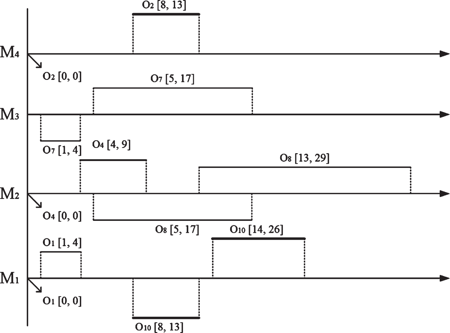
Gantt chart of the scheduling example with interval processing time.

3.2 Mathematical model

The IRPPS model presented in this study focuses on three conflicting objectives, that is, minimizing energy consumption, makespan, and maximum machine load, and deals with the trade-offs among them.

3.2.1 Notations and assumptions

To represent the IRPPS model, the following notations and assumptions are used:

Notations
P _n	the nth part, , where N is the number of parts
F _i	the ith feature, , where I is the number of features in the part
FM _ik	the kth failure mode of F_i, , where K_i is the number of failure modes of F_i
O _nj	the jth operation to P_n, , where J_n is the number of features that need to be reprocessed in part P_n and is equal to the number of operations to P_n
O _l	the lth operation, , where L is the number of operations
M _s	the sth machine, , where S is the number of machines
$\tilde{E}$	the total interval energy consumption
${\tilde{E}}_{p}$	the total interval processing energy consumption
${\tilde{E}}_{idle}$	the total interval idle energy consumption
${\tilde{T}}_{nj}^{s}$	the interval processing time of O_nj that is executed on M_s
${\tilde{ST}}_{nj}^{s}$	the interval start time of the O_nj on the M_s
${\tilde{CT}}_{nj}^{s}$	the interval completion time of O_nj on the M_s
$W_{p}^{s}$	the unit processing power of the M_s
$W_{idle}^{s}$	the unit idle power of the M_s
H _s	the time threshold to turn off M_s
$X_{ni}^{k}$	0-1 decision variable, with 1 indicating that F_i of part P_n has FM_ik, and 0 otherwise
$Y_{ni}^{l}$	0-1 decision variable, with 1 indicating that F_i of P_n is reprocessed by O_l, and 0 otherwise
$β_{nj}^{l}$	0-1 decision variable, with 1 indicating that the F_i is selected as O_nj to process P_n, and 0 otherwise
$δ_{nj}^{s}$	0-1 decision variable, with 1 indicating that O_nj is executed on M_s, and 0 otherwise
$χ_{n^{'} j^{'} nj}^{s}$	0-1 decision variable, with 1 indicating that O_n′j′ and O_nj are adjacent operations executed on M_s, and O_n′j′ precedes O_nj, and 0 otherwise
$σ_{n^{'} j^{'} nj}^{s}$	0-1 decision variable, with 1 indicating that M_s is turned off between adjacent operations O_n′j′ and O_nj (O_n′j′ precedes O_nj) on it, and 0 otherwise
$α_{nj}^{s}$	0-1 decision variable, with 1 indicating that O_nj is the first to be executed on M_s, and 0 otherwise

Assumptions

(1) All parts and features are independent of each other.

(2) All parts have no priority.

(3) All parts and machines are available at the beginning.

(4) All interruptions are ignored.

(5) All transportation times can be ignored.

(6) Each part can only be processed by one machine at a time, and multiple features of the same part cannot be reprocessed simultaneously.

(7) The setup times for the machines are assumed to be negligible.

(8) The energy consumption of the auxiliary equipment is ignored.

(9) The machine startup and shutdown times are ignored.

(10) Infinite buffers and no blocking are considered.

(11) Each operation can be processed on at least one machine.

3.2.2 Formula of the IRPPS model

(1) Objective function for the total energy consumption

In this IRPPS model, the total energy consumption consists of two parts: total interval processing energy consumption and total interval idle energy consumption. In addition, the turn-on/off mode is applied in this model to reduce energy consumption. Inspired by Wu and Sun [33] and Lei et al. [39], to reduce the complexity of the proposed model, the machine needs to be turned off if its idle time exceeds a given time threshold. For example, H_s = 7 means that machine M_s needs to be turned off if its idle time exceeds 7 h.

The total interval processing energy consumption ${\tilde{E}}_{p}$ is calculated using Equation (5): ${\tilde{E}}_{p} = \sum_{s = 1}^{S} \sum_{n = 1}^{N} \sum_{j = 1}^{J_{n}} W_{p}^{s} \cdot δ_{nj}^{s} \cdot ({\tilde{CT}}_{nj}^{s} ⊖ {\tilde{ST}}_{nj}^{s})$ (5)

The variable used to determine the total interval idle energy consumption is calculated using Equation (6) and ${\tilde{E}}_{idle}$ is calculated using Equation (7): $σ_{n^{'} j^{'} nj}^{s} = {\begin{matrix} 1 {\tilde{ST}}_{nj}^{s} ⊖ {\tilde{CT}}_{n^{'} j^{'}}^{s} > H_{s} \\ 0 {\tilde{ST}}_{nj}^{s} ⊖ {\tilde{CT}}_{n^{'} j^{'}}^{s} \leq H_{s} \end{matrix}$ (6) $\begin{matrix} {\tilde{E}}_{idle} = \sum_{s = 1}^{S} \sum_{n = 1}^{N} \sum_{n^{'} = 1}^{N} \sum_{j = 1}^{J_{n}} \sum_{j^{'} = 1}^{J_{n^{'}}} W_{idle}^{s} \cdot χ_{n^{'} j^{'} nj}^{s} \cdot \\ ({\tilde{ST}}_{nj}^{s} ⊖ {\tilde{CT}}_{n^{'} j^{'}}^{s}) \cdot (1 - σ_{n^{'} j^{'} nj}^{s}) \end{matrix}$ (7) where Equation (6) checks whether M_s can be turned off between two adjacent operations.

The objective function of the total interval energy consumption is calculated using Equation (8): ${\tilde{f}}_{1} = \tilde{E} = {\tilde{E}}_{p} \oplus {\tilde{E}}_{idle}$ (8)

(2) Objective function for the interval makespan

The variables used to determine the makespan are calculated using Equations (9) and (10), as follows: ${\tilde{ST}}_{nj}^{s} = {\begin{matrix} 0 & α_{nj}^{s} = 1, j = 1 \\ {\tilde{CT}}_{n (j - 1)}^{s^{'}} & α_{nj}^{s} = 1, j > 1 \\ {\tilde{CT}}_{n^{'} j^{'}}^{s} & α_{nj}^{s} = 0, j = 1 \\ max ({\tilde{CT}}_{n (j - 1)}^{s^{'}}, {\tilde{CT}}_{n^{'} j^{'}}^{s}) & α_{nj}^{s} = 0, j > 1 \end{matrix}$ (9) ${\tilde{CT}}_{nj}^{s} = {\tilde{ST}}_{nj}^{s} \oplus {\tilde{T}}_{nj}^{s}$ (10) where Equations (9) and (10) represent, respectively, the interval start time and interval completion time of O_nj on M_s, ${\tilde{CT}}_{n (j - 1)}^{s^{'}}$ represents the interval completion time of O_n(j-1) on $M_{s}^{'}$ , and ${\tilde{CT}}_{n^{'} j^{'}}^{s}$ represents the interval completion time of the previous adjacent operation executed on M_s prior to O_nj.

The objective function of interval makespan is calculated by Equation (11): ${\tilde{f}}_{2} = max_{1 \leq n \leq N} (\sum_{s = 1}^{S} {\tilde{CT}}_{{nJ}_{n}}^{s})$ (11) where ${\tilde{CT}}_{{nJ}_{n}}^{s}$ is the interval completion time of O_{nJ
_n} on the M_s.

(3) Objective function for the maximum machine load

In the IRPPS model, the maximum machine load is calculated using Equation (12): ${\tilde{f}}_{3} = max_{1 \leq s \leq S} {\sum_{n = 1}^{N} \sum_{j = 1}^{J_{n}} δ_{nj}^{s} \cdot ({\tilde{CT}}_{nj}^{s} ⊖ {\tilde{ST}}_{nj}^{s})}$ (12)

(4) Objectives and constraints

The standard multiple optimization objectives of the IRPPS model are formalized as Equation (13): $F = {\begin{matrix} Minimise (\tilde{f_{1}}) \\ Minimise (\tilde{f_{2}}) \\ Minimise (\tilde{f_{3}}) \end{matrix}$ (13)

The below constraints need be taken into consideration to achieve the aforementioned objectives: $\sum_{i = 1}^{I} \sum_{k = 1}^{K_{i}} X_{ni}^{k} = J_{n}$ (14) $\sum_{l = 1}^{L} \sum_{i = 1}^{I} Y_{ni}^{l} = J_{n}$ (15) $\sum_{s = 1}^{S} δ_{nj}^{s} = 1, \forall j and \forall n$ (16) $\sum_{l = 1}^{L} β_{nj}^{l} = 1, \forall j and \forall n$ (17) where Equation (14) ensures that each defective feature in a part fails owing to one failure mode, Equation (15) indicates that each defective feature can only be reprocessed by one operation, Equation (16) shows that each operation can only be executed on one machine, and Equation (17) indicates that only one O_l in the operation set is selected as O_nj to process P_n.

(5) Equivalent transformation of objective function value

According to Li et al. [10], the mean and variance of the interval numbers can be calculated using Equations (18) and (19), respectively, which are then used to transform the interval objective value into the real value using Equation (20). $M (\tilde{f_{m}}) = \frac{f_{m}^{L} + f_{m}^{R}}{2}$ (18) $σ^{2} (\tilde{f_{m}}) = \frac{{(f_{m}^{L})}^{2} + {(f_{m}^{R})}^{2} - 2 f_{m}^{L} \cdot f_{m}^{R}}{12}$ (19) $\begin{matrix} R [{\tilde{f}}_{m}] = M ({\tilde{f}}_{m}) + ω_{m} \cdot σ ({\tilde{f}}_{m}) \\ = \frac{f_{m}^{L} + f_{m}^{R}}{2} + ω_{m} \cdot \frac{f_{m}^{R} - f_{m}^{L}}{\sqrt{12}} \end{matrix}$ (20) where $f_{m}^{L}$ and $f_{m}^{R}$ represent the lower and upper bounds of objective value ${\tilde{f}}_{m}$ , respectively. $R [{\tilde{f}}_{m}]$ indicates the real value after equivalent transformation, and ω _m (the value is between 0 and 1) is the weight of the uncertainty (i.e., variance) of the objective function m. ω _m can be adjusted according to the requests of real remanufacturing environments.

4 ENSGA-II for the IRPPS model

This section introduces the basic NSGA-II and explores the proposed ENSGA-II.

4.1 The basic NSGA-II

The NSGA-II proposed by Deb et al. [11] has become a widely recognized method for optimizing multi-objective problems in the last two decades. To provide better convergence capabilities and maintain population diversity, the NSGA-II integrates fast non-dominated sorting and crowding distance approaches, which are briefly introduced as follows.

4.1.1 Fast non-dominated sorting

Fast non-dominated sorting is an effective approach for achieving better convergence capabilities. In a multi-objective optimization problem, conflicts may be produced among different objectives. When one objective value improves, the others may worsen. Thus, the fast non-dominated sorting is employed to classify all solutions into different non-dominated ranks. Solutions with lower non-dominated ranks dominate those with higher non-dominated ranks, and the solutions with the same non-dominated rank are not dominated by each other.

4.1.2 Crowding distance (CD)

CD is a common method for keeping the diversity of solutions that equips NSGA-II with lower computational complexities and can be employed to obtain a uniformly spreading Pareto-optimal solution set. The crowded-comparison operator is employed to select the solutions. It is defined as follows: if the solutions are of the same non-domination rank, a higher CD value is preferable. The interval CD is calculated using Equation (21) [22]. $m_{i} = \frac{[f_{m}^{L}, f_{m}^{R}]^{i + 1} - [f_{m}^{L}, f_{m}^{R}]^{i - 1}}{(f_{m}^{C_{max}} + f_{m}^{W_{max}}) - (f_{m}^{C_{min}} - f_{m}^{W_{min}})}$ (21) where $[D_{L}, D_{R}]_{m}^{i}$ is the interval CD of solution i under objective function m. $f_{m}^{C_{max}}$ and $f_{m}^{C_{min}}$ denote the maximum and minimum mid-points of the solutions under objective function m, respectively. $f_{m}^{W_{max}}$ and $f_{m}^{W_{min}}$ represent the maximum and minimum half-widths of the solutions under objective function m, respectively.

4.2 The proposed ENSGA-II

The uncertain IRPPS problem can be considered a hybrid problem that is divided into the remanufacturing process plan selection sub-problem and scheduling sub-problem. On the basis of Section 4.1, the ENSGA-II is proposed to obtain optimal solutions in the uncertain IRPPS model. Three improvements are made to the basic NSGA-II framework in this study: (1) a new multi-dimensional representation scheme is designed to comprehensively characterize the solutions; (2) a new self-adaptive strategy and multiple genetic operators are integrated to increase the diversity of the population; and (3) a new local search strategy is employed to avoid premature convergence and enhance algorithmic exploration.

In Fig. 2, the framework of the ENSGA-II is presented, where N represents the initial population size. P^G and O^G represent the parent and offspring populations in the Gth generation, respectively.

Fig. 2

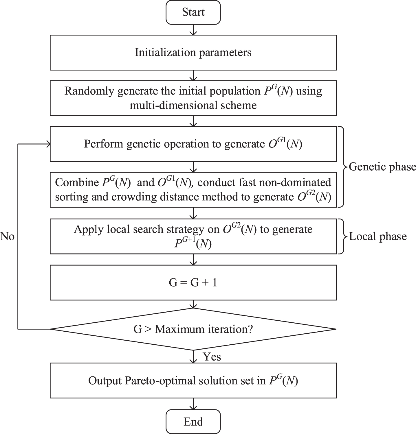
The framework of the ENSGA-II.

4.2.1 Encoding

An efficient encoding scheme is an important part of connecting mathematical models and optimization algorithms. Considering the characteristics of the uncertain IRPPS model, a chromosome should reflect both the information and processing flexibility of the parts. To effectively characterize the IRPPS model, a multi-dimensional representation scheme is proposed.

The multi-dimensional representation scheme comprises two layers: a feature layer and a reprocessing layer. The former includes the part index, features, and failure mode information (i.e., the first dimension), while the latter includes a candidate operation string (i.e., the second dimension) and candidate machine string (i.e., the third dimension). Based on the illustrated flexible process plans shown in Table 1, an example is given to demonstrate the multi-dimensional representation scheme (Fig. 3).

Each value in the first dimension represents a defective feature of one part that fails owing to a failure mode, and the length in this dimension indicates the cumulative number of all defective features of all parts that need to be reprocessed. For example, the last value [4 , 1], indicates that defective feature 5 of part 4 fails owing to failure mode 1 (FM₅₁).

Each value in the second dimension represents the rth candidate operation that is selected to reprocess the corresponding defective feature. For example, the last value 2 indicates that the second candidate operation (i.e., O₆) is selected to reprocess the above defective feature [4 , 1].

Each value in the third dimension represents the qth candidate machine selected to execute the corresponding operation. For example, the last value 1 indicates that O₆ is executed on the first candidate machine (i.e., M₃).

Fig. 3

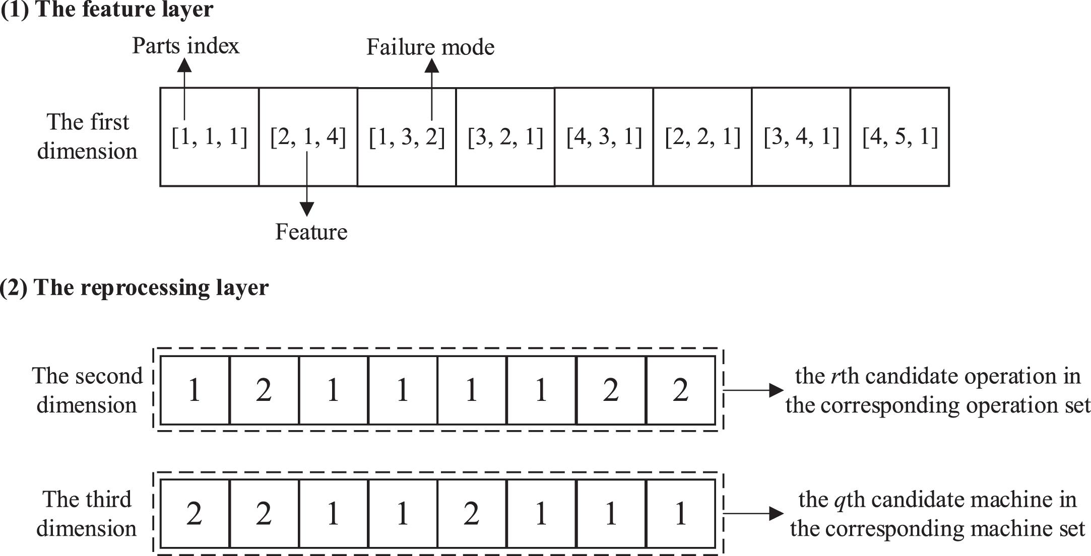
An example of the multi-dimensional representation scheme.

4.2.2 Crossover operators

The precedence operation crossover (POX) and job-based order crossover (JOX) [40] are extended with the proposed multi-dimensional representation scheme, and then randomly selected as the crossover operator to generate the offspring.

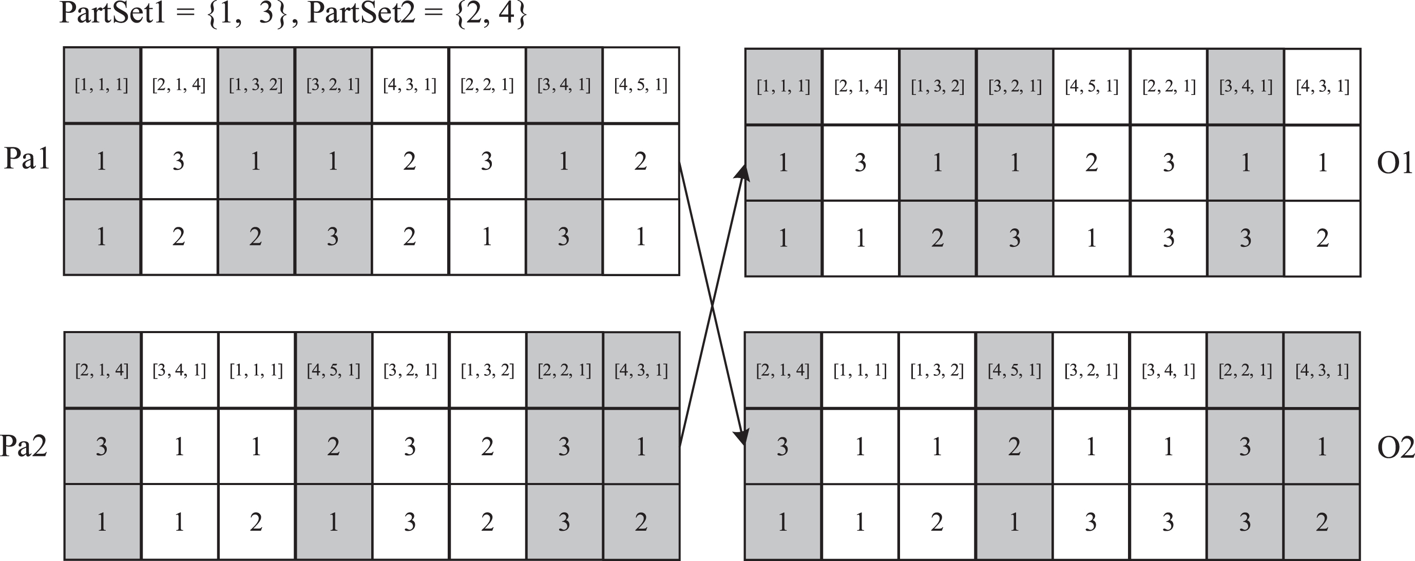
Figure 4 shows an example of the extended POX operator. Detailed steps are listed below:

Randomly divide all the part numbers {1, . . . , n, . . . , N}, into two non-empty sets, PartSet1 and PartSet2.

Duplicate the genes from parent1 (Pa1) and parent2 (Pa2) whose part numbers belong to PartSet1 into offspring1 (O1) and offspring2 (O2), respectively, at the same position.

Duplicate the genes from Pa1 and Pa2 whose part numbers belong to PartSet2 into O2 and O1, respectively, and maintain their precedence order.

Fig. 4

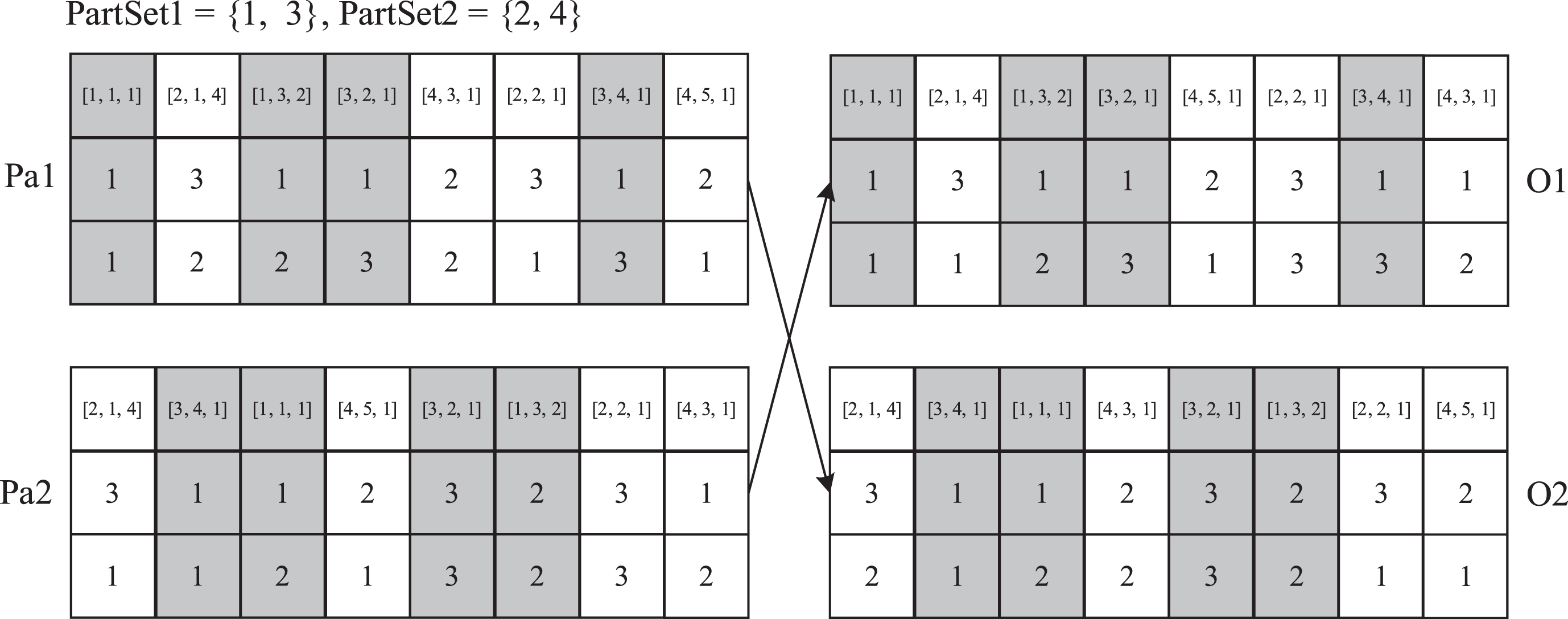
An example of the extended POX operator.

Figure 5 shows an example of the extended JOX operator. Detailed steps are listed below:

Randomly divide all the part numbers {1, . . . , n, . . . , N} into two non-empty sets, PartSet1 and PartSet2.

Duplicate the genes from parent1 (Pa1) whose part numbers belong to PartSet1 into offspring1 (O1), and duplicate the genes from parent2 (Pa2) whose part numbers belong to PartSet2 into O2 at the same position.

Duplicate the genes from Pa1 whose part numbers belong to PartSet1 into O2, duplicate the genes from Pa2 whose part numbers belong to PartSet2 into O1, and maintain their precedence order.

Fig. 5

An example of the extended JOX operator.

In this study, a self-adaptive strategy for crossover probability P_c is proposed for the crossover operation, as shown in Equation (22), where P_{c_initial} is the initial crossover probability, iter_max and iter_current represent the maximum iteration and current iteration, respectively. $P_{c} = P_{c_initial} \times e^{- \frac{iter_current}{iter_max}}$ (22)

4.2.3 Mutation operator

The two-point swapping operator is used to mutate the feature layer, and the single-point mutation operator is used to mutate the reprocessing layer.

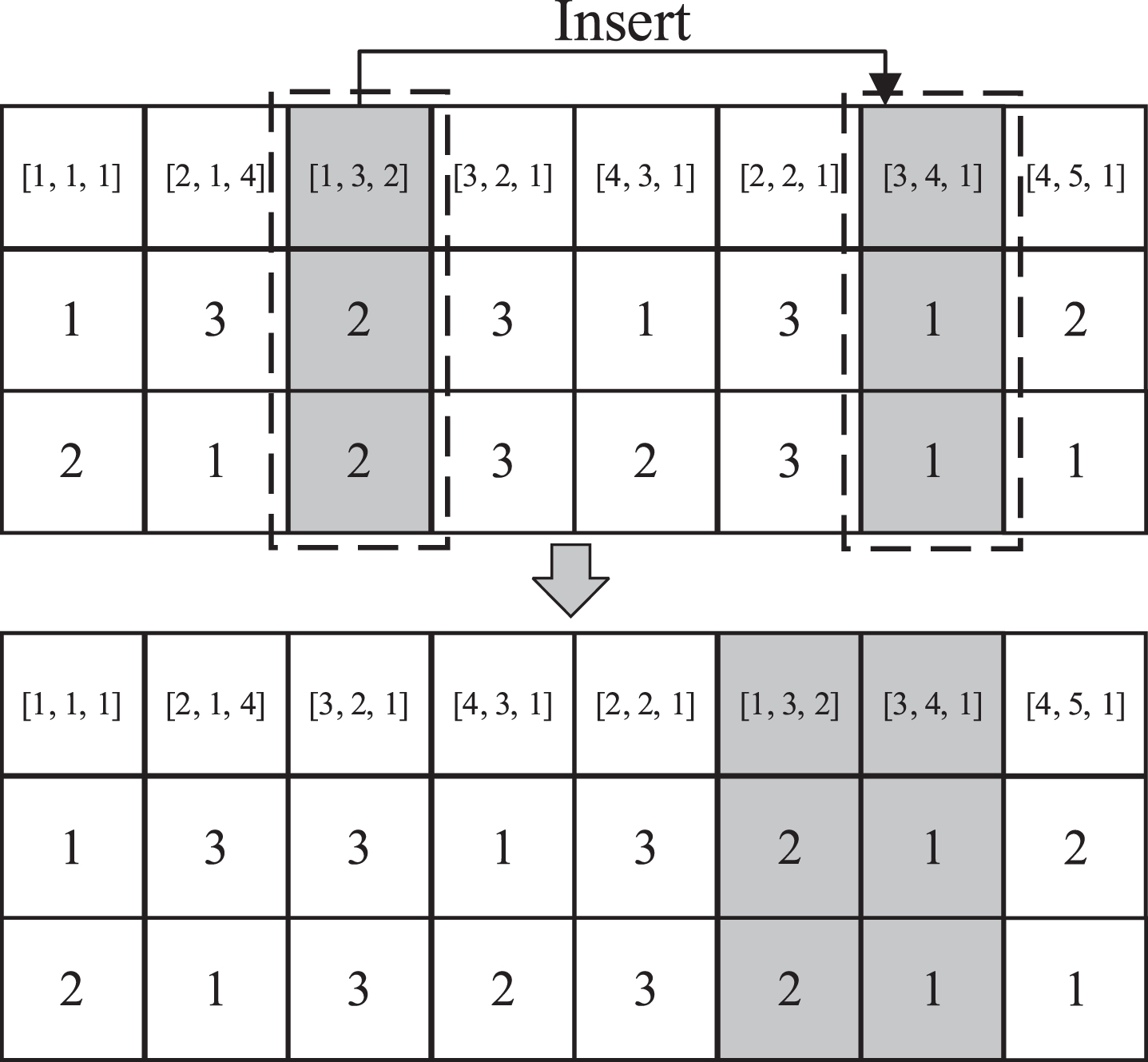
For the two-point swapping operator, Fig. 6 shows an example of randomly selecting two points and swapping the corresponding genes.

For the single-point mutation operator, randomly select one point and replace the gene with a different gene in the candidate set, and do nothing if there is only one gene in the candidate set.

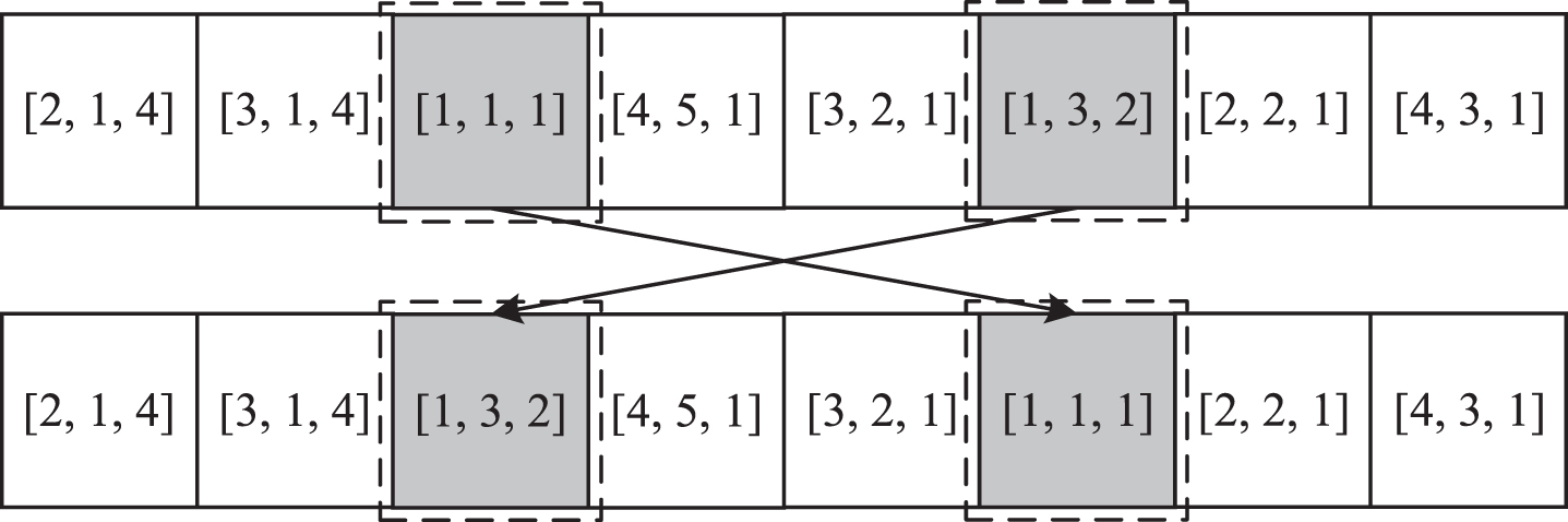
In this study, a self-adaptive strategy for mutation probability P_m is proposed for mutation operation, as shown in Equation (23), where P_{m_initial} denotes the initial mutation probability. $P_{m} = P_{m_initial} \times e^{- \frac{iter_current}{iter_max}}$ (23)

Fig. 6

An example of performing the two-point swapping operator.

4.2.4 Local search strategy

To avoid premature convergence and improve algorithmic exploration, a local search strategy that includes four local search operators is employed to extend the basic NSGA-II algorithm. The first local search operator (LS1) is designed to find a better process plan for each part. The second local search operator (LS2) aims to find a new process plan and generate a scheduling scheme that is better than the current one. The third local search operator (LS3) aims to jump out of the local optimal solution to avoid premature convergence. The fourth local search operator (LS4) is designed to ameliorate the quality of solutions and repair the infeasible solutions obtained by LS3. The above four local search operators are described below.

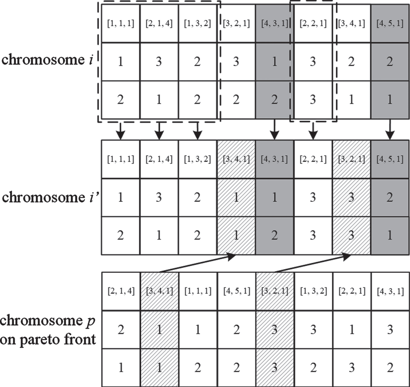
LS1: The process plan of each part depends on the order of the defective features in the feature layer. Figure 7 shows an illustrative example, and detailed steps are listed below:

Fig. 7

An example of performing LS1.

Compare the feature order of each part between chromosomes i and p. Because the feature orders of P₁ (i.e., F₁ are followed by F₃) and P₂ (i.e., F₁ are followed by F₂) are the same between chromosomes i and p, they are kept unchanged at the same position in the new chromosome i’.

Because the feature orders of P₃ and P₄ are different between chromosomes i and p, about half of the parts with the corresponding features (i.e., P₄ with F₃ followed by F₅) are kept unchanged at the same position in the new chromosome i’.

Duplicate the remained parts with the corresponding features (i.e., P₃ with F₄ followed by F₂) from chromosome p to the new chromosome i’, with their precedence order unchanged.

LS2: LS2 is performed on the reprocessing layer to find a new process plan and generate a new scheduling scheme. Figure 8 shows an illustrative example, and detailed steps are listed below:

Randomly select chromosome i in the population and generate a string vector H with 0 and 1, with the same length as the chromosome i.

The genes in the reprocessing layer corresponding to element 1 in the string vector H are kept unchanged at the same position in the new chromosome i’.

The two dimensions in the reprocessing layer of chromosome i represent the selection of candidate operations and candidate machines, respectively. Replace the operation genes corresponding to element 0 in the string vector H with another candidate operation and replace the machine genes with another machine with the shortest processing time in the new chromosome i’.

Fig. 8

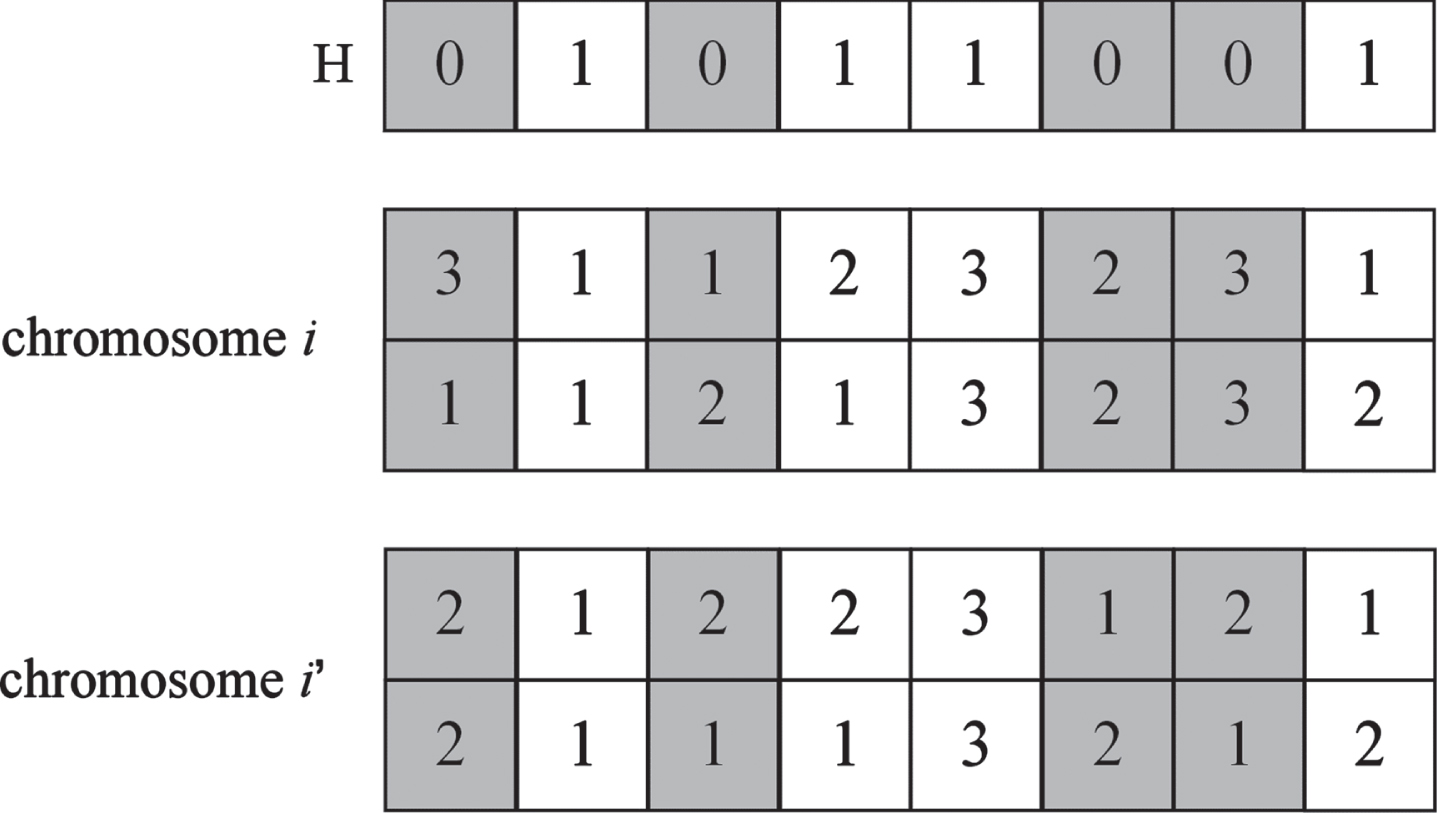
An example of performing LS2 on reprocessing layer.

LS3: LS3 is an insertion operator. Two different genes are randomly chosen, and the former is inserted before the latter to make them adjacent. Figure 9 shows an illustrative example.

LS4: Performing LS3 may result in infeasible solutions; for example, the feature layer might not meet the feature constraints, and the selected operation or machine might not fulfill the corresponding part or operation. Thus, LS4 is designed to repair infeasible solutions. Detailed steps are listed below:

Fig. 9

An example of performing LS3.

Repair of the feature layer. According to the feature constraints, check whether the feature order of each part meets the feature constraints. If one does not, randomly reorganize the feature genes belonging to the part to satisfy the feature constraints.

Repair of the reprocessing layer. According to the repaired feature layer, check whether the corresponding operations and machines can fulfill the required functions. If one does not, randomly select a feasible operation or machine gene in the corresponding candidate set to fulfill the required function.

The pseudocode of the local search strategy is shown in Algorithm 1, where R1, R2, and R3 represent the selection probabilities of LS1, LS2, and LS3, respectively.

Algorithm 1: Local search strategy
Input: a chromosome i
Output: an updated chromosome
1: i ← 0
2: whilei < 10 do
3: generate a random number v between [0, 1]
4: ifv < R1
5: i ’ ← perform the LS1 on i
6: ifi ’ dominates i
7: i ← i ’
8: end if
9: end if
10: ifR1< = v< R1 + R2
11: i^′′← perform the LS2 on i
12: ifi ” dominates i
13: i ← i ”
14: end if
15: end if
16: ifR1 + R2< = v< = R1 + R2 + R3
17: i ”’ ← perform the LS3 on i
18: ifi ”’ dominates i
19: i ← i ”’
20: end if
21: end if
22: end while
23: Return an updated chromosome

The pseudocode of the ENSGA-II is shown in Algorithm 2.

Algorithm 2: ENSGA-II
Input: Maximum iteration: Maxiter, population
Output: Pareto-optimal solution set
1: G ← 0
2: NP₁, NP₂ ←Ø
3. whileG < Maxiterdo
4: determine the crossover and mutation probabilities according to Equations (22) and (23), respectively
5: perform crossover and mutation operators on population P^G (N) to generate offspring population O^G1 (N)
6: NP1 ←O^G1 (N) ⋃ P^G (N)
7: perform fast non-dominated sorting and crowding distance method on NP1 to generate new population O^G2 (N)
8: perform the local search strategy on O^G2 (N) to generate NP2
9: G = G+1
10: P^G (N)← NP2
11: end while
12: Return Pareto-optimal solution set in P^G (N)

5 Simulation experiments

Simulation experiments were conducted in this section to evaluate the performance of ENSGA-II. NSGA-II [34], strength Pareto evolutionary algorithm-2 (SPEA2) [41], and MOPSO [26] are Pareto-based multi-objective algorithms that have been widely used to solve multi-objective scheduling problems. Therefore, the proposed ENSGA-II was compared to the three other baseline multi-objective algorithms, i.e., the NSGA-II, SPEA2, and MOPSO, whose pseudocodes are shown in Algorithms 3–5, respectively. All the experimental simulations were performed in a Python environment on a personal computer with a 64-bit version of Windows 10, an Intel (R) Core with a CPU speed of 3.10 GHz, and 16 GB RAM.

Algorithm 3: NSGA-II
Input: Maximum iteration: Maxiter, initial population: P⁰ (N)
Output: Pareto-optimal solution set
1: g ← 0
2. whileg < Maxiterdo
3: perform crossover and mutation operators to obtain offspring population O^g (N)
4: C^g (2N) ← P^g (N) ⋃ O^g (N)
5: sort C^g (2N) with fast non-dominated sorting and crowding distance, then select the first N chromosome to form P^g+1 (N)
6: g = g + 1
7: end while
8: Return Pareto-optimal solution set

Algorithm 4: SPEA2
Input: Maximum iteration: Maxiter, archive size: $\bar{N}$ , population size: N
Output: Pareto-optimal solution set: A
1: t ← 0
2: generate an initial population P₀ and create the empty archive $\bar{P_{0}}$
3. whilet < Maxiter do
4: calculate fitness values of individuals in P_t and ${\bar{P}}_{t}$
5: copy all nondominated individuals in P_t and ${\bar{P}}_{t}$ to ${\bar{P}}_{t + 1}$
6: if size of ${\bar{P}}_{t + 1}$ > $\bar{N}$
7: reduce ${\bar{P}}_{t + 1}$ with the truncation operator
8: else
9: fill ${\bar{P}}_{t + 1}$ with dominated individuals in P_t and ${\bar{P}}_{t}$
10: perform binary tournament selection with replacement on ${\bar{P}}_{t + 1}$ in order to fill the mating pool
11: apply recombination and mutation operators to the mating pool and set ${\bar{P}}_{t + 1}$ to the resulting population
12: set A to the set of decision vectors represented by the nondominated individuals in ${\bar{P}}_{t + 1}$
13: t = t + 1
14: end while
15: Return set A

Algorithm 5: MOPSO
Input: Maximum iteration: Maxiter, initial population
Output: Pareto-optimal solution set
1: g ← 0
2: use heuristic rules to initialize population, all archives, personal-best positions and global-best position
3. whileg < Maxiterdo
4: generate a new position based on the position update formula
5: generate a random number rand between [0, 1]
6: ifrand < perturbation operator probability
7: execute perturbation operator
8: else
9: update personal-best archives and global-best archive with non-dominated archive update strategy
10: perform variable neighborhood search on global-best archive
11: update the personal-best positions and the global-best position
12: g = g + 1
13: end while
14: Return Pareto-optimal solution set

5.1 Experimental design

To simulate the real remanufacturing environment, the experimental data and parameters were defined as follows. In each instance, the number of parts, which varied from 4 to 30, and the machine number, which ranged from 6 to 12, were randomly generated. The benchmark data of the parts are listed in Table 2, including the feature number range, the operation number, the number of feature constraints, and applicable parts. In addition, the specific feature constraints and other illustrative properties can be found in the literature given in the “Adopted from” column of Table 2. For each feature, the number of failure modes, which varied from 1 to 4, was randomly generated, as was the number of candidate operations for each failure mode and the number of candidate machines for each operation, which both ranged from 1 to 3. The parameters listed in Table 3 were also randomly generated within the corresponding ranges. All experimental data utilized in this study is publicly accessible through Figshare database (https://doi.org/10.6084/m9.figshare.16746637). For each instance in the database, the name includes the total number of parts, the benchmark dataset ID, and the total number of machines. For example, the “Exp (4/1/6)” indicates the total number of parts was 4, the benchmark dataset was #1, and the total number of machines was 6. To reduce accidental errors in experiments, each experiment was conducted 10 times independently and the results were averaged to obtain the final experimental results.

Table 2
Benchmark datasets of parts

ID of Feature Operation Adopted Number of Applicable parts

datasets number number from feature constraints

1 [1, 7] 9 Table 9 of Li et al. [42] 1 /

2 [1, 8] 21 Table 6 of Li et al. [40] 5 packaging machine

3 [1, 14] 18 Table 11 of Li et al. [42] 8 /

4 [1, 10] 15 Table 1 of Li et al. [40] 7 packaging machine

ID of	Feature	Operation	Adopted	Number of	Applicable parts
1	[1, 7]	9	Table 9 of Li et al. [42]	1	/
2	[1, 8]	21	Table 6 of Li et al. [40]	5	packaging machine
3	[1, 14]	18	Table 11 of Li et al. [42]	8	/
4	[1, 10]	15	Table 1 of Li et al. [40]	7	packaging machine

Table 3

The parameters for experiments

Variable	Value	Unit	Type
$W_{p}^{s}$	[8, 25]	kw	Integer
$W_{idle}^{s}$	[1, 3]	kw	Integer
H _s	[6, 9]	h	Integer
${\tilde{T}}_{nj}^{s}$	[5, 20](mid-point)	h	Integer
	[1, 2](half-width)	h	Integer
ω₁/ω₂/ω₃	0.5/0.5/0.5		Decimal

5.2 Performance metrics

To evaluate the proposed ENSGA-II comprehensively, three multi-objective algorithm evaluation indicators, namely, the set coverage [43], spacing [44], and hypervolume [43] indicators are adopted.

(1) Set coverage (SC)

The SC indicator was designed to evaluate the convergence of the Pareto-optimal solution set produced by the various multi-objective algorithms, as shown in Equation (24). $SC (U, V) = \frac{| {u \in U | \exists ν \in V : ν ≻ u} |}{| U |}$ (24) where U and V are two Pareto-optimal solution sets. SC(U, V) is used to measure the proportion of solutions in set V dominated by those in set U. |U| represents the solution number in set U. SC(U, V) = 1 indicates that all the solutions in V are dominated by those in U. SC(U, V) = 0 means that all the solutions in set V are not dominated by any one in set U. The closer the value of SC(U, V) is to 0, the better the convergence of the solutions in set U.

(2) Spacing indicator (SI)

The SI measures the distribution or spreading of solutions over the Pareto-optimal solution set, and are defined in Equations (25) and (26): $SI = \sqrt{\frac{1}{NS} \sum_{i = 1}^{NS} (d_{i} - \bar{d})^{2}}$ (25) $d_{i} = \min_{j} \sum_{m = 1}^{M} | f_{m}^{i} - f_{m}^{j} | (i \neq j, i, j = 1,, N S)$ (26) where NS and M are the number of solutions in the Pareto-optimal solution set and the number of objective functions, respectively. $\bar{d}$ represents the average value of d_i calculated using Equation (26), where $f_{m}^{i}$ denotes the mth objective value of the solution i. The closer to zero the SI is, the more uniform the Pareto-optimal solution is.

(3) Hypervolume (HV)

The HV indicator is utilized to comprehensively evaluate the convergence and distribution of the multi-objective algorithms, which is defined in Equation (27). $\begin{matrix} HV (U, R) = Volume \\ (\underset{i \in U}{\cup} \times [f_{2}^{i}, r_{2}] \times \dots \times [f_{m}^{i}, r_{m}]) \end{matrix}$ (27) where the reference point in the objective space is R = (r₁, r₂, …, r_m) ^T. $[f_{m}^{i}, r_{m}]$ denotes the distance between $f_{m}^{i}$ in set U and r_m. HV(U, R) denotes the volume of the objective space, which uses R as the boundary and is dominated by set U. The larger the HV(U, R) is, the better the performance of set U is.

5.3 Parameter design

The maximum number of iterations was set to 300 for all algorithms. As the HV indicator comprehensively measures the performance of algorithms, it was used for sensitivity analysis of the parameters in the proposed ENSGA-II, including the selection probability of performing local search operators and population size.

The first experiment, Exp (15/1/8), tested the performance of ENSGA-II with different combinations of selection probabilities of local search operators (LS1, LS2, and LS3). In this experiment, the initial population size was fixed at 40. Table 4 shows 13 selection probability combinations of local search operators used for this experiment.

Table 4
Selection probability combinations of local search operators

Combinations LS1 LS2 LS3

C01 1/3 1/3 1/3

C02 0.8 0.1 0.1

C03 0.1 0.8 0.1

C04 0.1 0.1 0.8

C05 0.6 0.3 0.1

C06 0.1 0.6 0.3

C07 0.3 0.1 0.6

C08 0.4 0.4 0.2

C09 0.2 0.4 0.4

C10 0.4 0.2 0.4

C11 0.3 0.6 0.1

C12 0.1 0.3 0.6

C13 0.6 0.1 0.3

Combinations	LS1	LS2	LS3
C01	1/3	1/3	1/3
C02	0.8	0.1	0.1
C03	0.1	0.8	0.1
C04	0.1	0.1	0.8
C05	0.6	0.3	0.1
C06	0.1	0.6	0.3
C07	0.3	0.1	0.6
C08	0.4	0.4	0.2
C09	0.2	0.4	0.4
C10	0.4	0.2	0.4
C11	0.3	0.6	0.1
C12	0.1	0.3	0.6
C13	0.6	0.1	0.3

The HV values produced by ENSGA-II under various combinations of local search operator selection probabilities are shown in Fig. 10. It can be observed that the HV value of C06 is higher than that of the other combinations; therefore, the combinations of selection probabilities of local search operators are set as 0.1, 0.6, and 0.3, respectively, in the experiments that followed.

Fig. 10

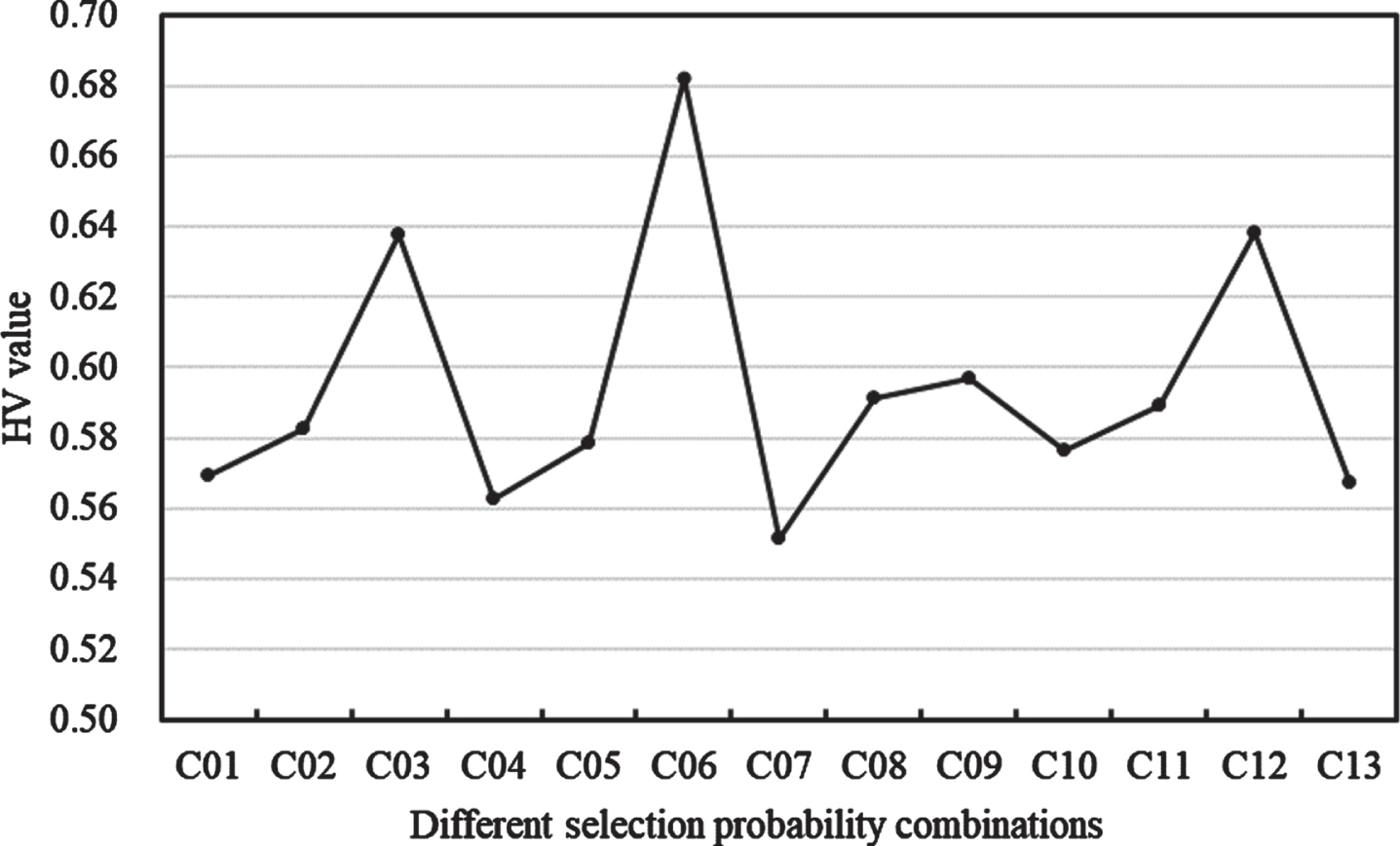
The HV values corresponding to various selection probability combinations.

The second experiment tested the HV values of ENSGA-II with different population sizes on differently scaled datasets. Figure 11 shows that the HV value changes slowly when the initial population size exceeds 40. As large population sizes increase the computational cost associated with the simulations, the initial population size is set to 40 in the experiments that follow. This population size also ensures that an efficient comparison could be made.

Fig. 11

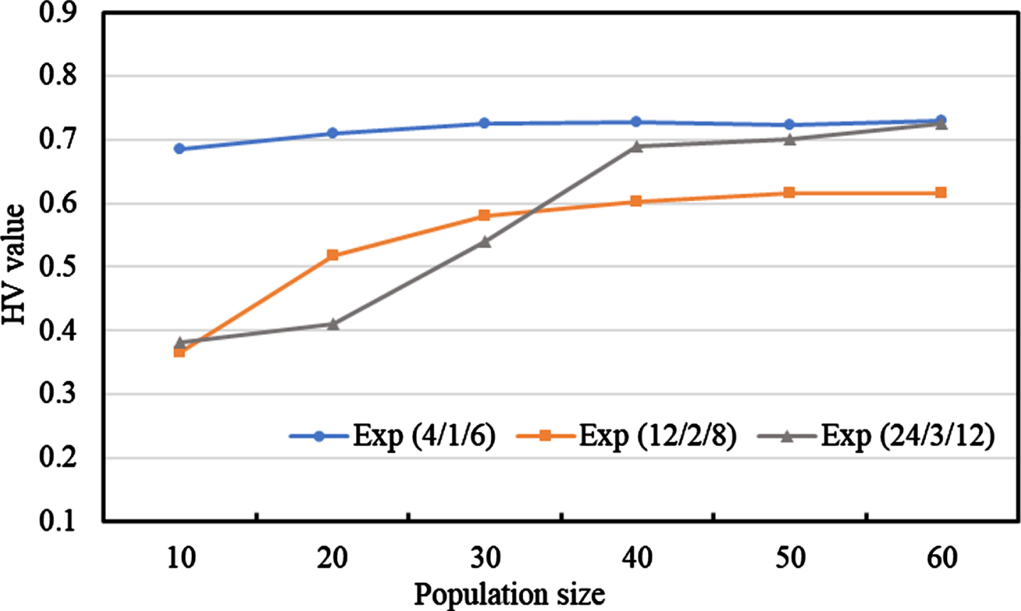
The HV values corresponding to different population sizes.

To make a fair comparison between ENSGA-II and three other baseline algorithms, the number of local search operators executed in the ENSGA-II and NSGA-II, as well as the number of neighborhoods in the MOPSO were all set to 10. Table 5 lists the other parameters of the multi-objective algorithms after the trial run.

Table 5

The other parameters of multi-objective algorithms

Algorithm	Parameters
ENSGA-II	initial crossover probability P_{c_initial} = 0.9
	initial mutation probability P_{m_initial} = 0.3
NSGA-II	maximal self-adaption probabilities = 0.9
	minimal self-adaption probabilities = 0.2
SPEA2	crossover rate = 0.7
	archive size = 30
	mutation rate = 0.3
MOPSO	probability of current position impact = 0.98
	probability of executing the perturbation
	operator = 0.02
	probability of personal-best position impact = 0.6
	probability of global-best position impact = 0.4
	maximum size of personal-best archive = 5
	maximum size of global-best archive = 15

5.4 Comparison of ENSGA-II with other baseline multi-objective algorithms

In the following experiments, the performance comparison between the ENSGA-II and those of other baseline multi-objective algorithms, including the NSGA-II, SPEA2, and MOPSO, are evaluated comprehensively. Tables 6, 7, and 8 (better results are boldfaced) show the comparative results based on the SC, SI, and HV, respectively.

Table 6 compares the results of the SC indicator obtained by four algorithms. It is found that in all conducted experiments, the ENSGA-II demonstrates superior performance over other baseline algorithms significantly. The second and third columns reveal that at least one solution obtained by ENSGA-II dominates all the solutions obtained by NSGA-II in most of the experiments, while the solutions obtained by NSGA-II do not dominate any solution obtained by ENSGA-II. The fourth and fifth columns reveal that at least one solution obtained by ENSGA-II dominates all the solutions obtained by SPEA2, while the solutions obtained by SPEA2 do not dominate any solution obtained by ENSGA-II. The sixth and seventh columns reveal that at least one solution obtained by ENSGA-II dominates the partial solutions obtained by MOPSO, while the solutions obtained by MOPSO do not dominate any solution obtained by ENSGA-II in most of the experiments.

Table 7 compares the results of the SI obtained by four algorithms. It shows that the Pareto-optimal solution set obtained by ENSGA-II exhibits a more uniform distribution than those obtained with the baseline algorithms in most of the experiments.

Table 8 compares the results of the HV indicator obtained by four algorithms. The reference point R = (1, 1, 1) ^T. As shown in Table 8, the majority of experimental results indicate that the ENSGA-II generates the significantly higher HV values than the baseline algorithms. According to the results, the solutions obtained by the ENSGA-II exhibit better convergence and distribution compared to those obtained by the baseline algorithms.

Table 6
The SC comparisons among four algorithms

Datasets	Instance	ENSGA-II(E) vs. NSGA-II(N)		ENSGA-II(E) vs. SPEA2(S)		ENSGA-II(E) vs. MOPSO(P)
		SC(E, N)	SC(N, E)	SC(E, S)	SC(S, E)	SC(E, P)	SC(P, E)
#1	Exp(4/1/6)	1.000000	0.000000	1.000000	0.000000	0.844301	0.042615
	Exp(8/1/10)	1.000000	0.000000	1.000000	0.000000	1.000000	0.000000
	Exp(10/1/9)	1.000000	0.000000	1.000000	0.000000	0.961095	0.000000
	Exp(15/1/8)	0.989286	0.000000	1.000000	0.000000	0.871282	0.036430
	Exp(21/1/10)	1.000000	0.000000	1.000000	0.000000	0.829425	0.000000
	Exp(30/1/10)	1.000000	0.000000	1.000000	0.000000	1.000000	0.000000
#2	Exp(5/2/9)	1.000000	0.000000	1.000000	0.000000	0.972174	0.006174
	Exp(7/2/8)	1.000000	0.000000	1.000000	0.000000	1.000000	0.000000
	Exp(12/2/8)	1.000000	0.000000	1.000000	0.000000	0.966667	0.002703
	Exp(17/2/12)	1.000000	0.000000	1.000000	0.000000	1.000000	0.000000
	Exp(22/2/9)	1.000000	0.000000	1.000000	0.000000	0.926326	0.000000
	Exp(25/2/8)	1.000000	0.000000	1.000000	0.000000	0.994309	0.000000
#3	Exp(6/3/12)	1.000000	0.000000	1.000000	0.000000	1.000000	0.000000
	Exp(9/3/9)	1.000000	0.000000	1.000000	0.000000	1.000000	0.000000
	Exp(16/3/7)	1.000000	0.000000	1.000000	0.000000	0.921951	0.000000
	Exp(18/3/6)	1.000000	0.000000	1.000000	0.000000	1.000000	0.000000
	Exp(20/3/10)	1.000000	0.000000	1.000000	0.000000	1.000000	0.000000
	Exp(24/3/12)	1.000000	0.000000	1.000000	0.000000	1.000000	0.000000
#4	Exp(4/4/7)	1.000000	0.000000	1.000000	0.000000	0.996875	0.000000
	Exp(6/4/6)	1.000000	0.000000	1.000000	0.000000	1.000000	0.000000
	Exp(10/4/8)	1.000000	0.000000	1.000000	0.000000	0.987500	0.002500
	Exp(14/4/10)	1.000000	0.000000	1.000000	0.000000	0.939333	0.000000
	Exp(16/4/9)	1.000000	0.000000	1.000000	0.000000	0.951515	0.008108
	Exp(25/4/12)	1.000000	0.000000	1.000000	0.000000	0.709910	0.108415

Table 7

The SI comparisons among four algorithms

Datasets	Instance	ENSGA-II	NSGA-II	SPEA2	MOPSO
		SI	SI	SI	SI
#1	Exp(4/1/6)	0.095259285	0.182785446	0.238554846	0.063515175
	Exp(8/1/10)	0.097462202	0.162229335	0.645587002	0.215177250
	Exp(10/1/9)	0.083998110	0.154805174	0.391207597	0.139251929
	Exp(15/1/8)	0.070590629	0.138952172	0.272538166	0.097193079
	Exp(21/1/10)	0.073801098	0.134812601	0.174956721	0.116251240
	Exp(30/1/10)	0.067238341	0.078308009	0.199714464	0.072724763
#2	Exp(5/2/9)	0.093865006	0.246931727	0.162459721	0.172838317
	Exp(7/2/8)	0.094529682	0.153771126	0.326422058	0.180439905
	Exp(12/2/8)	0.096259986	0.108418556	0.214818409	0.101932489
	Exp(17/2/12)	0.059209242	0.081100628	0.332665773	0.156562340
	Exp(22/2/9)	0.093380363	0.151538265	0.193708784	0.127477396
	Exp(25/2/8)	0.071470030	0.085567821	0.178588993	0.137684095
#3	Exp(6/3/12)	0.088668820	0.131831757	0.269848934	0.118016976
	Exp(9/3/9)	0.085242897	0.084227198	0.184084461	0.110297266
	Exp(16/3/7)	0.056364522	0.060686459	0.142665619	0.054173407
	Exp(18/3/6)	0.086136742	0.104475521	0.326420970	0.106182368
	Exp(24/3/12)	0.071266100	0.117984636	0.161104697	0.138717204
	Exp(20/3/10)	0.057448312	0.193073742	0.116654767	0.090968744
#4	Exp(4/4/7)	0.128057498	0.116161498	0.418119516	0.142958298
	Exp(6/4/6)	0.115156077	0.138540243	0.326230377	0.135307203
	Exp(10/4/8)	0.079195864	0.140224593	0.187502585	0.140251842
	Exp(14/4/10)	0.069855563	0.096131131	0.180536059	0.073138298
	Exp(16/4/9)	0.054368778	0.126777383	0.295420718	0.147425073
	Exp(25/4/12)	0.081002590	0.159269566	0.156524149	0.188390488

Table 8

The HV comparisons among four algorithms

Datasets	Instance	ENSGA-II	NSGA-II	SPEA2	MOPSO
		HV	HV	HV	HV
#1	Exp(4/1/6)	0.727661003	0.703032474	0.293996597	0.770048931
	Exp(8/1/10)	0.778014910	0.532640321	0.232163632	0.597760451
	Exp(10/1/9)	0.669972408	0.546620031	0.346943422	0.584318183
	Exp(15/1/8)	0.681861079	0.594668907	0.431517176	0.583149634
	Exp(21/1/10)	0.559333320	0.500353976	0.463040313	0.537927206
	Exp(30/1/10)	0.575843330	0.478823886	0.354226177	0.491332611
#2	Exp(5/2/9)	0.696527634	0.695870740	0.500400519	0.668218480
	Exp(7/2/8)	0.680549376	0.613334753	0.498982259	0.625839740
	Exp(12/2/8)	0.602936530	0.557723801	0.448973481	0.575535848
	Exp(17/2/12)	0.636869370	0.574374938	0.417724924	0.547776581
	Exp(22/2/9)	0.622499491	0.574892249	0.509935664	0.653036670
	Exp(25/2/8)	0.625313533	0.517135159	0.537084138	0.529314989
#3	Exp(6/3/12)	0.653466205	0.628038391	0.319359704	0.624731261
	Exp(9/3/9)	0.669518195	0.654028879	0.365704028	0.562733581
	Exp(16/3/7)	0.516178811	0.454832435	0.504899623	0.474640576
	Exp(18/3/6)	0.688517094	0.586658474	0.277007181	0.602786532
	Exp(20/3/10)	0.510741868	0.505339743	0.427428627	0.454583765
	Exp(24/3/12)	0.690040764	0.510764106	0.491402232	0.531193973
#4	Exp(4/4/7)	0.646268486	0.628316443	0.406620860	0.644835450
	Exp(6/4/6)	0.735586625	0.666183038	0.419530402	0.692138274
	Exp(10/4/8)	0.600322725	0.543441336	0.328901311	0.555322284
	Exp(14/4/10)	0.743877809	0.693180196	0.559141786	0.659368820
	Exp(16/4/9)	0.587034873	0.462012059	0.389672696	0.523181215
	Exp(25/4/12)	0.640356092	0.621320349	0.379008989	0.535583840

Figure 12 shows box plots based on the comparative results in Tables 6–8, respectively. It is observed that the performance and stability of the ENSGA-II are superior to those of the baseline algorithms.

Fig. 12

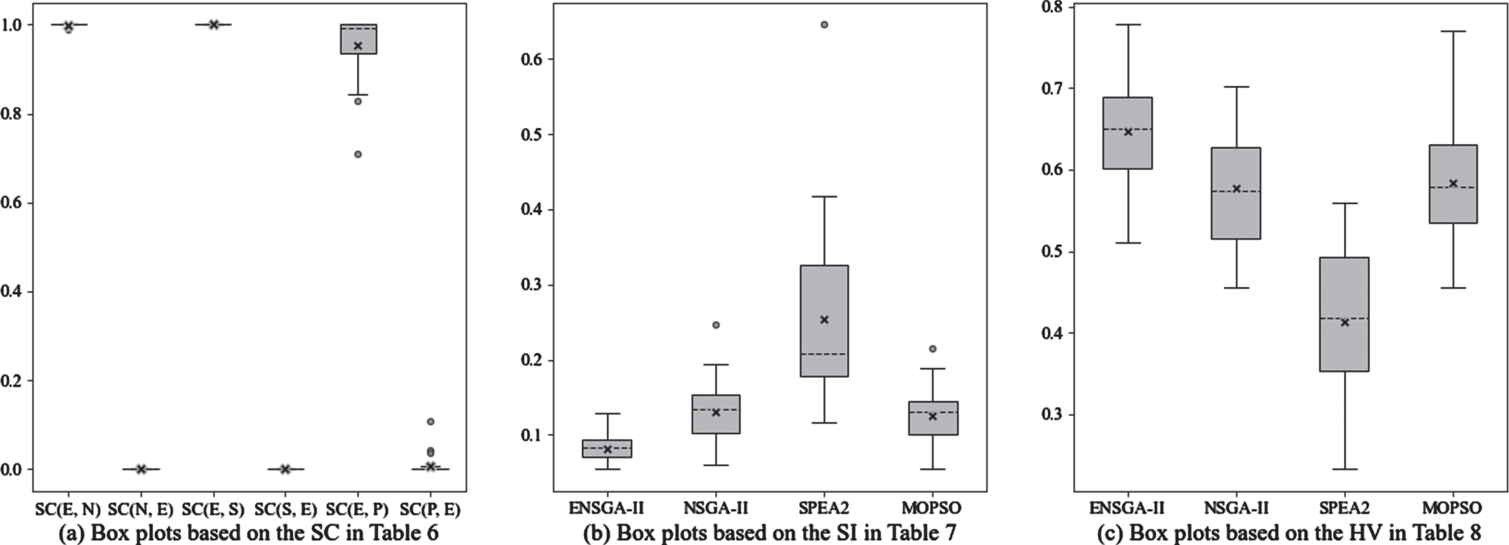
Box plots based on the experimental results.

To make the experimental results more intuitive, Fig. 13 reveals the Pareto-optimal solution sets produced by four algorithms. The majority of solutions produced by the baseline algorithms are dominated by the solutions produced by the ENSGA-II. Moreover, the solution set obtained by the ENSGA-II outperforms those of the baseline algorithms on the convergence and distribution in experiments with different scales. Besides, when the scale of the test instance increases, the ENSGA-II exhibits an excellent performance and reaches the Pareto-optimal solution set more easily than other baseline algorithms.

Fig. 13

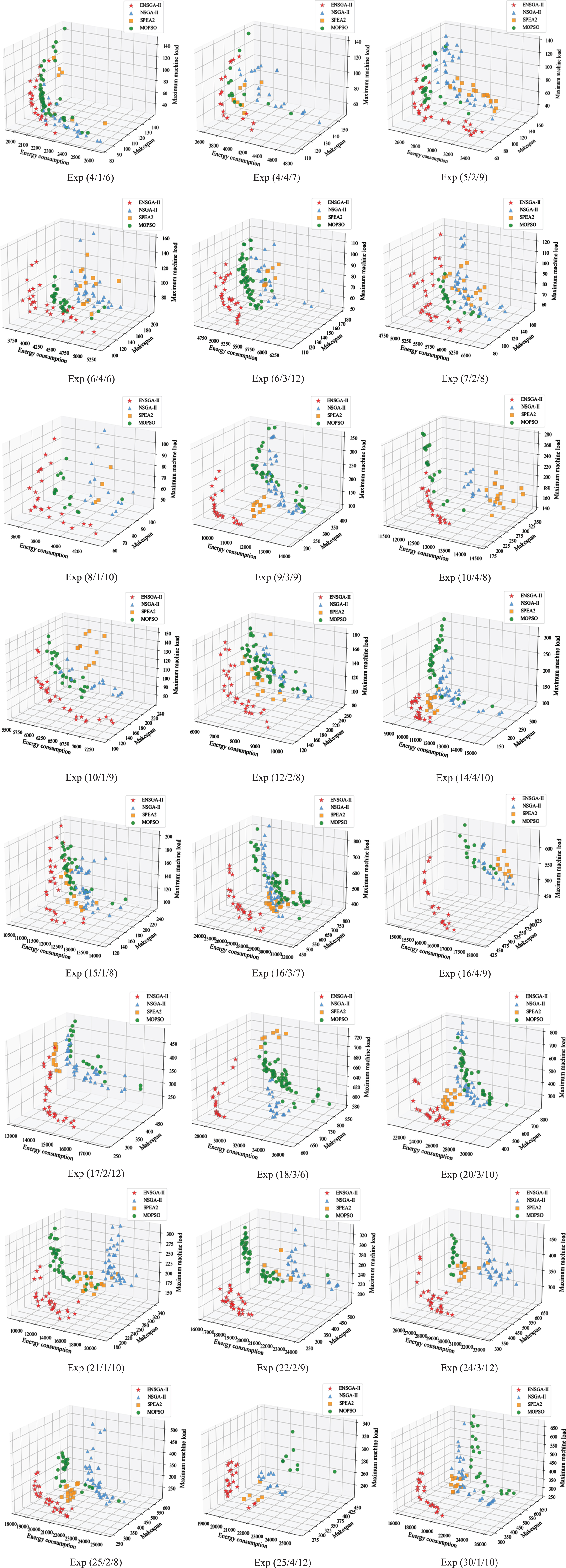
The Pareto-optimal solution sets produced by four algorithms.

In the case of instance Exp(4/4/7), Table 9 shows a set of Pareto solutions obtained by ENSGA-II and the three other baseline algorithms. The findings reveal that the solutions derived from ENSGA-II with three objectives consistently outperform those obtained by the three other baseline algorithms. Such superiority is attributed to the fact that every solution produced by each baseline algorithm is dominated by at least one solution generated by ENSGA-II.

Table 9

The Pareto optimal solutions of four algorithms on the instance Exp(4/4/7)

Solution	ENSGA-II			NSGA-II			SPEA2			MOPSO
	$\tilde{f_{1}}$	$\tilde{f_{2}}$	$\tilde{f_{3}}$	$\tilde{f_{1}}$	$\tilde{f_{2}}$	$\tilde{f_{3}}$	$\tilde{f_{1}}$	$\tilde{f_{2}}$	$\tilde{f_{3}}$	$\tilde{f_{1}}$	$\tilde{f_{2}}$	$\tilde{f_{3}}$
1	[2642, 4204]	[92, 132]	[80, 112]	[2792, 4302]	[91, 147]	[72, 128]	[2857, 4349]	[118, 160]	[51, 95]	[2869, 4385]	[85, 127]	[70, 98]
2	[2788, 4282]	[87, 125]	[60, 84]	[2943, 4465]	[109, 149]	[75, 85]	[2857, 4349]	[101, 143]	[58, 106]	[2804, 4338]	[88, 130]	[80, 112]
3	[2593, 4141]	[100, 160]	[90, 126]	[3590, 5122]	[108, 148]	[56, 70]	[2865, 4355]	[95, 139]	[58, 106]	[2666, 4228]	[104, 150]	[100, 140]
4	[2996, 4506]	[93, 129]	[50, 62]	[2823, 4353]	[117, 161]	[80, 112]	[2870, 4366]	[93, 129]	[51, 95]	[2731, 4275]	[94, 136]	[90, 126]
5	[2776, 4350]	[80, 122]	[58, 108]	[2884, 4436]	[95, 141]	[65, 117]	[2859, 4377]	[86, 134]	[51, 95]	[2796, 4322]	[91, 133]	[80, 112]
6	[2761, 4257]	[86, 126]	[70, 98]	[2831, 4349]	[110, 150]	[80, 112]	[2982, 4484]	[88, 126]	[75, 85]	[2926, 4416]	[100, 136]	[75, 85]
7	[2596, 4144]	[101, 147]	[90, 126]	[2900, 4412]	[90, 138]	[72, 128]	[3045, 4549]	[88, 126]	[51, 95]	[2861, 4369]	[88, 130]	[70, 98]
8	[2771, 4363]	[80, 122]	[60, 84]	[3114, 4702]	[102, 146]	[51, 97]	[3077, 4575]	[88, 126]	[44, 84]	[2926, 4416]	[85, 127]	[58, 106]
9	[3172, 4758]	[85, 125]	[37, 75]	[2819, 4357]	[114, 158]	[80, 112]				[2601, 4181]	[114, 164]	[110, 154]
10	[3166, 4682]	[88, 126]	[40, 56]	[3598, 5126]	[104, 146]	[56, 70]				[2953, 4447]	[85, 127]	[75, 85]
11	[2596, 4164]	[93, 149]	[90, 126]	[2853, 4329]	[111, 155]	[65, 117]				[3027, 4533]	[85, 127]	[51, 95]
12	[2859, 4335]	[83, 123]	[60, 68]	[3281, 4889]	[100, 150]	[44, 86]				[3486, 5088]	[101, 137]	[56, 76]
13	[2952, 4532]	[95, 133]	[37, 75]	[2923, 4431]	[125, 173]	[58, 106]				[3163, 4681]	[102, 144]	[44, 84]
14	[2779, 4353]	[80, 122]	[51, 97]	[3316, 4870]	[106, 142]	[44, 84]
15	[2579, 4155]	[94, 154]	[90, 126]	[3785, 5291]	[110, 150]	[40, 60]
16	[2845, 4337]	[83, 123]	[44, 84]	[3582, 5130]	[105, 147]	[56, 70]
17	[3112, 4620]	[87, 125]	[37, 73]	[3168, 4764]	[99, 151]	[60, 68]
18				[3005, 4593]	[93, 147]	[75, 85]
19				[2937, 4441]	[128, 170]	[58, 106]
20				[3035, 4723]	[86, 138]	[51, 99]

6 Conclusion

With the depletion of resources and the worsening of environmental pollution, remanufacturing has gained significant attention from various sectors as an environmentally friendly approach to sustainable development. In the remanufacturing process, process planning and scheduling plays an important role in actual remanufacturing applications. To effectively cope with the intrinsic uncertainties of the remanufacturing environment, a new IRPPS model under uncertainties was proposed and solved using the ENSGA-II. This study contributes to existing remanufacturing research through the following three main aspects.

A new IRPPS model with the objective of minimizing energy consumption, makespan, and maximum machine load is proposed. It applies interval numbers to represent the uncertainty of processing time and develops a process planning approach that integrates various failure modes to obtain a more practical and effective process plan and scheduling scheme.

To effectively optimize the IRPPS model, the ENSGA-II was proposed by integrating a new multi-dimensional representation scheme, a new self-adaptive strategy, and a new local search strategy.

Experiments were simulated to compare four algorithms in order to comprehensively evaluate the performance of the ENSGA-II in tackling the IRPPS model. The experiments were conducted on 24 sets of instances, showing that ENSGA-II outperforms three other baseline algorithms for all SC metrics, 83.3% for SI metrics, and 91.7% for HV metrics.

In addition, this study has the following deficiencies. In terms of modeling, there is a lack of application in actual remanufacturing cases and analysis of practical factors such as finite buffers and priority differences. In terms of algorithms, the applicability of the proposed algorithm to other scheduling models needs to be explored.

In the future, the following directions can be explored to further refine this study. First, the proposed model should be applied to an actual remanufacturing case and more larger-scale instances. Second, more practical factors should be considered in the proposed model. Furthermore, the issue of machine learning-based search strategies is intriguing and has the potential to enhance the applicability of ENSGA-II to other scheduling models.

Footnotes

Acknowledgments

This work has been supported by National Natural Science Foundation of China (No. 51975512), Philosophy and Social Science Program of Zhejiang Province (No. 21NDJC105YB), and Natural Science Foundation of Xinjiang Province (No. 2021D01A70).

Data availability statement

All experimental data for this research have been public in the Figshare database (https://doi.org/10.6084/m9.figshare.16746637).

Compliance with ethical standards

Conflicts of interest

The authors declare that there is no conflict of interests regarding the publication of this article.

Ethical standard

The authors state that this research complies with ethical standards. This research does not involve either human participants or animals.

References

Gong

G.L.

, Deng

Q.W.

, Chiong

, Gong

X.R.

, Huang

H.Z.Y.

and Han

W.W.

, Remanufacturing-oriented process planning and scheduling: mathematical modelling and evolutionary optimisation, International Journal of Production Research 58(12) (2020), 3781–3799.

W.Y.

, Zhang

C.X.

, Liu

C.H.

and Liu

, Error propagation model and optimal control method for the quality of remanufacturing assembly, Journal of Intelligent & Fuzzy Systems 42(3) (2022), 2533–2547.

Guide

V.D.R.

Jr , Production planning and control for remanufacturing: industry practice and research needs, Journal of Operations Management 18(4) (2000), 467–483.

Baptista

, Barbosa-Póvoa

A.P.

, Escudero

L.F.

, Gomes

M.I.

and Pizarro

, On risk management of a two-stage stochastic mixed 0-1 model for the closed-loop supply chain design problem, European Journal of Operational Research 274(1) (2019), 91–107.

X.Y.

and Chen

W.D.

, Optimal ordering and production decisions for remanufacturing firms with carbon options under demand uncertainty, Environmental Science and Pollution Research 30(12) (2023), 34378–34393.

Shi

J.X.

, Zhang

W.Y.

, Zhang

, Wang

W.R.

, Lin

and Feng

R.J.

, A new environment-aware scheduling method for remanufacturing system with non-dedicated reprocessing lines using improved flower pollination algorithm, Journal of Manufacturing Systems 57 (2020), 94–108.

Petrović

, Vuković

, Mitić

and Miljković

, Integration of process planning and scheduling using chaotic particle swarm optimization algorithm, Expert Systems with Applications 64 (2016), 569–588.

Wang

, Jiang

Z.G.

, Zhang

X.G.

, Wang

Y.N.

and Wang

, A fault feature characterization based method for remanufacturing process planning optimization, Journal of Cleaner Production 161 (2017), 708–719.

Zhang

W.K.

, Zheng

Y.F.

and Ahmad

, An energy-efficient multi-objective scheduling for flexible job-shop-type remanufacturing system, Journal of Manufacturing Systems 66 (2023), 211–232.

10.

X.Y.

, Gao

, Wang

W.W.

, Wang

C.Y.

and Wen

, Particle swarm optimization hybridized with genetic algorithm for uncertain integrated process planning and scheduling with interval processing time, Computers & Industrial Engineering 135 (2019), 1036–1046.

11.

Deb

, Pratap

, Agarwal

and Meyarivan

, A fast and elitist multiobjective genetic algorithm: NSGA-II, IEEE Transactions on Evolutionary Computation 6(2) (2002), 182–197.

12.

Sheikhalishahi

, Eskandari

, Mashayekhi

and Azadeh

, Multi-objective open shop scheduling by considering human error and preventive maintenance, Applied Mathematical Modelling 67 (2019), 573–587.

13.

Gheitasi

, Feylizadeh

M.R.

and Ahari

R.M.

, A multi-objective mathematical model of financial flows in Omni-Channel distribution systems, Journal of Intelligent &Fuzzy Systems 42(6) (2022), 4851–4879.

14.

Deng

S.K.

, Xiao

C.Y.

, Zhu

Y.K.

, Peng

J.Y.

, Li

and Liu

Z.H.

, High-frequency direction forecasting and simulation trading of the crude oil futures using Ichimoku KinkoHyo and Fuzzy Rough Set, Expert Systems with Applications 215 119326. (2023).

15.

Zhang

W.Y.

, Wang

, Liu

X.Q.

and Zhang

, A new uncertain remanufacturing scheduling model with rework risk using hybrid optimization algorithm, Environmental Science and Pollution Research 30 62744–62761. (2023).

16.

Wang

W.J.

, Tian

G.D.

, Zhang

H.H.

, Li

Z.W.

and Zhang

L.L.

, A hybrid genetic algorithm with multiple decoding methods for energy-aware remanufacturing system scheduling problem, Robotics and Computer-Integrated Manufacturing 81 102509. (2023).

17.

Guo

, Zou

J.F.

, Du

B.G.

and Wang

K.P.

, Integrated scheduling for remanufacturing system considering component commonality using improved multi-objective genetic algorithm, Industrial Engineering 182 109419. (2023).

18.

Zhang

, Ong

S.K.

and Nee

A.Y.C.

, A simulation-based genetic algorithm approach for remanufacturing process planning and scheduling, Applied Soft Computing 37 (2015), 521–532.

19.

Zhang

W.K.

, Zheng

Y.F.

, Ahmad

The integrated process planning and scheduling of flexible job-shoptype remanufacturing systems using improved artificial bee colony algorithm, Journal of Intelligent Manufacturing (2022). DOI:10.1007/s10845-022-01969-2.

20.

Zhang

W.K.

, Zheng

Y.F.

and Ahmad

, An energy-efficient multi-objective integrated process planning and scheduling for a flexible job-shop-type remanufacturing system, Advanced Engineering Informatics 56 102010. (2023).

21.

Zhao

J.L.

, Peng

S.T.

, Li

, Lv

S.P.

, Li

M.Y.

and Zhang

H.C.

, Energy-aware fuzzy job-shop scheduling for engine remanufacturing at the multi-machine level, Frontiers of Mechanical Engineering 14(4) (2019), 474–488.

22.

Biswas

, Shaikh

A.A.

and Niaki

S.T.A.

, Multi-objective non-linear fixed charge transportation problem with multiple modes of transportation in crisp and interval environments, Applied Soft Computing 80 (2019), 628–649.

23.

Jamrus

, Chien

C.F.

, Gen

and Sethanan

, Hybrid particle swarm optimization combined with genetic operators for flexible job-shop scheduling under uncertain processing time for semiconductor manufacturing, IEEE Transactions on Semiconductor Manufacturing 31(1) (2017), 32–41.

24.

Fang

Y.L.

, Ming

, Li

M.Q.

, Liu

and Pham

D.T.

, Multi-objective evolutionary simulated annealing optimisation for mixed-model multi-robotic disassembly line balancing with interval processing time, International Journal of Production Research 58(3) (2020), 846–862.

25.

Bhunia

A.K.

and Samanta

S.S.

, A study of interval metric and its application in multi-objective optimization with interval objectives, Computers & Industrial Engineering 74 (2014), 169–178.

26.

Huang

, Tian

, Wang

and Ji

Z.C.

, Multi-objective flexible job-shop scheduling problem using modified discrete particle swarm optimization, SpringerPlus 5(1) (2016).

27.

Abed-Alguni

B.H.

and Alawad

N.A.

, Distributed Grey Wolf Optimizer for scheduling of workflow applications in cloud environments, Applied Soft Computing 102 107113. (2021).

28.

Wang

, Sheng

B.Y.

, Lu

Q.B.

, Yin

X.Y.

, Zhao

F.Y.

, Lu

X.C.

, Luo

R.P.

and Fu

G.C.

, A novel multi-objective optimization algorithm for the integrated scheduling of flexible job shops considering preventive maintenance activities and transportation processes, Soft Computing 25 (2021), 2863–2889.

29.

Alawad

N.A.

and Abed-alguni

B.H.

, Discrete island-based cuckoo search with highly disruptive polynomial mutation and opposition-based learning strategy for scheduling of workflow applications in cloud environments, Arabian Journal for Science and Engineering 46(4) (2021), 3213–3233.

30.

Bezdan

, Zivkovic

, Bacanin

, Strumberger

, Tuba

and Tuba

, Multi-objective task scheduling in cloud computing environment by hybridized bat algorithm, Journal of Intelligent & Fuzzy Systems 42(1) (2022), 411–423.

31.

, Huang

Y.X.

, Meng

L.L.

, Gao

, Zhang

and Zhou

J.J.

, A Pareto-based collaborative multi-objective optimization algorithm for energy-efficient scheduling of distributed permutation flow-shop with limited buffers, Robotics and Computer-Integrated Manufacturing 74 102277(2022).

32.

Liu

Y.Q.

, Li

H.Z.

, Zhu

J.W.

, Lin

Y.S.

and Lei

W.D.

, Multi-objective optimal scheduling of household appliances for demand side management using a hybrid heuristic algorithm, Energy 262 125460 (2023).

33.

X.L.

and Sun

Y.J.

, A green scheduling algorithm for flexible job shop with energy-saving measures, Journal of Cleaner Production 172 (2018), 3249–3264.

34.

Zhang

W.Y.

, Xiao

J.H.

, Zhang

, Lin

and Feng

R.J.

, A utility-aware multi-task scheduling method in cloud manufacturing using extended NSGA-II embedded with game theory, International Journal of Computer Integrated Manufacturing 34(2) (2021), 175–194.

35.

Yuan

M.H.

, Li

Y.D.

, Zhang

L.Z.

and Pei

F.Q.

, Research on intelligent workshop resource scheduling method based on improved NSGA-II algorithm, Robotics and Computer-Integrated Manufacturing 71 102141 (2021).

36.

Afsar

, Palacios

J.J.

, Puente

, Vela

C.R.

and Gonzalez-Rodriguez

, Multi-objective enhanced memetic algorithm for green job shop scheduling with uncertain times, Swarm and Evolutionary Computation 68 101016 (2022).

37.

Moscato

, Cotta

An accelerated introduction to memetic algorithms, Handbook of Metaheuristics, Springer, Cham (2019), 275–309.

38.

Wang

Y.J.

, Wang

G.G.

, Tian

F.M.

, Gong

D.W.

and Pedrycz

, Solving energy-efficient fuzzy hybrid flow-shop scheduling problem at a variable machine speed using an extended NSGA-II, Engineering Applications of Artificial Intelligence 121 105977 (2023).

39.

Lei

D.M.

, Li

and Wang

, A two-phase meta-heuristic for multiobjective flexible job shop scheduling problem with total energy consumption threshold, IEEE Transactions on Cybernetics 49(3) (2018), 1097–1109.

40.

X.Y.

, Gao

, Pan

Q.K.

, Wan

and Chao

K.M.

, An effective hybrid genetic algorithm and variable neighborhood search for integrated process planning and scheduling in a packaging machine workshop, IEEE Transactions on Systems, Man and Cybernetics: Systems 49(10) (2019), 1933–1945.

41.

Zitzler

, Laumanns

, Thiele

SPEA2: Improving the strength Pareto evolutionary algorithm, Technical Report, Swiss Federal Institute of Technology (ETH), Zurich, Switzerland, 103. (2001).

42.

X.Y.

, Gao

and Wen

X.Y.

, Application of an efficient modified particle swarm optimization algorithm for process planning, The International Journal of Advanced Manufacturing Technology 67(5) (2013), 1355–1369.

43.

Zitzler

and Thiele

, Multiobjective evolutionary algorithms: a comparative case study and the strength Pareto approach, IEEE Transactions on Evolutionary Computation 3(4) (1999), 257–271.

44.

Schott

J.R.

Fault Tolerant Design Using Single and Mmulticriteria Genetic Algorithm Optimization, Doctoral dissertation, Massachusetts Institute of Technology, Boston, MA, US. (1995).

A new integrated remanufacturing process planning and scheduling model under uncertainties using extended non-dominated sorting genetic algorithm-II

Abstract

Keywords

1 Introduction

2 Related work

2.1 Remanufacturing process planning and scheduling

2.2 Interval number theory

3.1 Problem description

3.2.1 Notations and assumptions

3.2.2 Formula of the IRPPS model

4.1 The basic NSGA-II

4.1.1 Fast non-dominated sorting

4.1.2 Crowding distance (CD)

5.1 Experimental design

Table 6 The SC comparisons among four algorithms

Footnotes

Acknowledgments

Data availability statement

Compliance with ethical standards

Conflicts of interest

Ethical standard

References

Table 6
The SC comparisons among four algorithms