Sage Journals: Discover world-class research

Abstract

Nowadays, the massive industrial data has effectively improved the performance of the data-driven deep learning Remaining Useful Life (RUL) prediction method. However, there are still problems of assigning fixed weights to features and only coarse-grained consideration at the sequence level. This paper proposes a Transformer-based end-to-end feature-level mask self-supervised learning method for RUL prediction. First, by proposing a fine-grained feature-level mask self-supervised learning method, the data at different time points under all features in a time window is sent to two parallel learning streams with and without random masks. The model can learn more fine-grained degradation information by comparing the information extracted by the two parallel streams. Instead of assigning fixed weights to different features, the abstract information extracted through the above process is invariable correlations between features, which has a good generalization to various situations under different working conditions. Then, the extracted information is encoded and decoded again using an asymmetric structure, and a fully connected network is used to build a mapping between the extracted information and the RUL. We conduct experiments on the public C-MAPSS datasets and show that the proposed method outperforms the other methods, and its advantages are more obvious in complex multi-working conditions.

Keywords

Remaining useful life prediction multi-working conditions self-supervised learning transformer feature-level mask

1. Introduction

In recent years, sensor technology and computing systems have made rapid progress. The predictive health management (PHM) has received increasing attention in many industrial applications. PHM is designed to improve reliability and availability and reduce equipment maintenance costs [1]. PHM can reduce equipment downtime and facilitate predictive maintenance by making plans prior to the onset of failures. A key task of PHM is to predict the RUL of equipment reliably [2]. By accurately predicting the RUL, operators can know in advance when the system will fail. So, the operations can avoid catastrophic failures by developing predictive maintenance plans. On the other hand, they can also reduce maintenance costs by reducing some unnecessary maintenance activities. Therefore, the prediction of RUL is of great significance to the research in this field [3].

According to the literature review, RUL prediction methods can be roughly divided into model-based and data-driven methods [4]. Model-based methods require accurate dynamic modeling of mechanical equipment or components to describe the degradation trend of components [5]. The degradation process is modeled by mathematical methods, which require a thorough understanding of the system’s physical structure and degradation process. With the larger scale of modern industrial equipment and more complex structure, the nonlinear relationship between various components turns out to be more complicated. It is difficult to use the model-based method to establish a dynamic RUL prediction model. Meanwhile, there are problems of poor adaptability and scalability for the model-based methods.

Nowadays, with the development of information technology, a large amount of historical data can be collected from multiple sensors during the operation of the systems, significantly promoting the development of data-driven methods. Unlike model-based methods, data-driven methods require less prior knowledge and have better generalization ability, so they have been widely used in industry [6]. Data-driven approaches can be further divided into machine learning approaches and deep learning approaches. Some machine learning methods have been used in RUL prediction, such as extreme learning machine (ELM) [7], artificial neural network (ANN) [8], hidden Markov model (HMM) [9], and support vector regression (SVR) [10]. However, lacking professional experience often leads to less reasonable screening and prediction results. Traditional machine learning methods do not particularly consider the temporal dependency of time series, which will also lead to inaccurate prediction results for RUL. On the contrary, the deep learning model has drawn much attention recently because of its strong ability to extract high-dimensional representation from time series automatically [11].

Among deep learning-based methods, recurrent neural networks (RNN), convolutional neural networks (CNN), and their variants and hybrid networks are widely used. As a deep learning method specially designed for sequence problems, RNN can extract useful and important information from previously processed data across time steps and integrate it into the current cell state to model sequence data [12]. However, due to the serial structure of RNN, it is key to retain the necessary information of all time steps during the calculation process, which naturally causes gradient disappearance and gradient explosion during training, which makes it difficult to train. In addition, there is the problem of long computing time and poor efficiency. Although the improved Long Short Term Memory (LSTM) [13, 14, 15] method and Gated Recurrent Unit (GRU) [16] method can alleviate the above problems when dealing with long-term sequences. The problem of losing relevant important historical information still exists because only the latest sequence information is concerned during mapping. CNN-based methods usually employ 1D convolution and pooling filters to extract temporal information along the time dimension. However, when extracting latent relationships in long time series, CNN needs to increase the size of the convolution kernel and the network depth to obtain a larger receptive field to capture longer time series [17], resulting in a complex and huge model. Therefore, CNNs, RNNs, and their hybrid networks are limited in extracting long-term sequence relationships.

Another problem that has been widely studied recently is that the time steps and features that are more relevant to degradation should be given greater weight in the RUL prediction. The attention mechanism is an effective way to learn this correlation [17]. Its purpose is to analyze the correlation between different parts of the sequence and pay different attention to different parts. It can be modeled without considering the distance of each part in the sequence. Attention mechanism has been widely applied in the image [18], natural language processing [19], timing modeling, and other applications. Some work attempts to apply attention mechanism to predict RUL in RNN/CNN structure [2, 3, 14]. However, when dealing with long time series, they still face the problems of high computational complexity and large receptive field. The Transformer network [20] was recently proposed to handle sequence modeling. Transformer block integrating the encoder, self-attention mechanism, and residual network can capture long-term dependencies efficiently and highly parallel. And it can easily adapt to different input sequence lengths. References [6, 17, 21, 22] capture the correlation between time points in the time dimension by using a transformer-based model and assigning different weights to different time points. Some references [17, 21, 22] note the different effects of different features on the degradation. Different weights are given to different features by methods such as the attention mechanism, which fully uses important information in the data and achieves good results in the RUL prediction. However, for the methods described above, there are still two deficiencies that need to be improved:

•
In the current methods, whether the temporal attention in Transformer or the channel attention, they all only consider correlations at the sequence level. In practice, different components are coupled with each other. Degradation information is contained in the variation of each component sensor and between the different component sensors. This information is helpful for RUL prediction. Therefore, if the correlation between each sequence is only considered coarse-grained and the prediction model is not designed for the correlation between feature points, the rich feature information in the multi-dimensional time series cannot be fully learned. This limits the model’s learning ability and affects the final prediction results.
•
Most methods assign uniform weights to features in the case of multiple working conditions, which do not consider the correlation between different features at different times and the variation of this correlation. In practical problems, mass sensor data are often collected under different working conditions. Under different working conditions, the importance of different features for system or equipment degradation is not invariable. For example, different working conditions will induce different forms of degradation, and the importance of different corresponding characteristics to degradation will also change. If such correlations and variations in correlations are ignored, the model’s learning performance and generalization performance will be restricted, especially when dealing with multi-condition problems.

Aiming at the two problems mentioned above, we propose an RUL prediction method of feature mask self-supervised assisted learning approach based on Transformer (FMSL). First, the input features are subjected to self-supervised learning. Unlike the traditional method, which only considers the correlation between the entire sequence, we specially design a feature-level mask block for the correlation between features in the feature dimension, randomly removing several features in the input features through the random mask. Then, it enters two learning streams formed by stacking Transformer encoding blocks with the original feature sequence and makes the model pay more attention to the correlation between feature levels through joint optimization with the final RUL prediction. Through the mask reconstruction task, the model can simultaneously consider the correlation between different features at different times, extract more fine-grained abstract semantic information, and improve the generalization of the model.

The main contributions can be summarized as follows:

•
An end-to-end prediction architecture is proposed, in which the self-supervised method is introduced for supervised RUL prediction. By designing a random mask and reconstruction learning task for fine-grained features, a self-supervised method is added to traditional supervised RUL prediction. Through the joint learning of the mask reconstruction task and RUL prediction task, the model is promoted to extract the fine-grained temporal dependency and inter-dimensional correlation of time series to obtain robust feature extraction ability.
•
A self-supervised learning method for the fine-grained feature-level mask reconstruction method is proposed, which randomly masks the data at different time points under all features in a time window. Then feature extraction is performed on the masked data using the encoder, forcing the model to learn the precise correlation between different time points under all features. This correlation is always stable under different working conditions and does not change easily, which greatly enhances the generalization ability of the model and makes the model perform well under multiple working conditions.
•
Experiments are conducted on the widely used C-MAPSS turbofan engine dataset to evaluate the proposed method. We conduct ablation experiments and compare the proposed method with other state-of-the-art methods. The results show that the proposed method can significantly improve prediction performance.

The rest of this article is organized as follows. Section 2 introduces the literature and works related to our proposed method. Section 3 describes the proposed approach in detail. Section 4 contains the details of the experimental setup, experimental results, and analysis. Finally, the discussion, conclusions, and future works of the research are presented in Section 5 and Section 6.
2. Related work

By modeling the functional relationship between the equipment degradation process and the condition monitoring data, the method based on deep learning can automatically capture the important feature information from the original data to achieve end-to-end prediction [17]. In this section, we will review deep learning-based methods such as CNN/RNN and the methods that apply attention mechanisms to RUL prediction.

Deep learning neural networks have the ability of automatic feature extraction and great nonlinear fitting [23]. Currently, CNN, RNN, and their variants or hybrid network methods are widely used in RUL prediction [2]. For instance, Wang et al. [24] proposed a data-driven Bi-directional Long Short Term Memory (BiLSTM) network. The method can fully learn sensor data’s forward and backward dependencies and reveal hidden degradation patterns under different working conditions through the visual analysis of hidden layers. Experiments on the CMAPSS data set show that BiLSTM is superior to other traditional RUL estimation methods. Li et al. [25] proposed a data-driven method based on a deep convolutional neural network (DCNN). As CNN obtains local information through convolution operations, the long-distance time feature information of the long-term sequence can be obtained by deepening the depth of the network. Experiments show that the proposed method achieves higher prediction accuracy than traditional CNN and RNN methods. Combining the advantages of CNN and LSTM, Kong et al. [26] proposed a feature extraction method that integrates CNN and LSTM to extract spatial and temporal features better. Because of the powerful ability of deep learning to extract feature information, RNN, CNN, and improved methods (such as BiLSTM and DCNN) have achieved good results in the RUL prediction. However, they will still suffer from the limitations of important feature loss, high time complexity, and oversized models when dealing with long-term sequences.

In recent years, methods based on attention mechanisms have become the main research direction of RUL prediction. CNN and RNN combine attention-based methods to enhance their prediction performance. Moreover, some transformer-based methods consider the different importance of time series and the effects of different feature sequences on degradation through an attention mechanism-based approach. Song et al. [27] proposed an attention mechanism method based on a Temporal Convolutional Network (TCN), which utilizes distributed attention to weigh different sensors and time steps, respectively. The time series is then used for information extraction. Zeng et al. [28] also proposed a method based on deep attention residual neural network (DARNN). It assigns different weights to feature sequences and time series by using channel attention and temporal attention, respectively. Then RUL is predicted by the deep residual network and RNN module. In contrast to the above methods that consider temporal and feature attention, respectively, Liu et al. [3] proposed a learnable feature-level attention method. The method proposed a parameter matrix that can learn continuously with the training process. Each eigenvalue in the 2D feature data is assigned a weight value. The RUL is then predicted by BiLSTM and CNN. With the development of the Transformer model, its powerful sequence feature extraction performance and parallel attention method provide a new idea for RUL prediction. Transformer-based methods are less affected by increasing sequence lengths. The model is calculated in parallel, which is efficient and does not generate an oversized model like the CNNs method. Zhang et al. [17] noticed the problem that the traditional Transformer considers the information of the time series and the feature sequence together, which affects the prediction accuracy. They proposed a method to separately pay attention to the time series and the feature sequence and fuse the extracted features to predict the RUL. Different from the attention method in [17], Liu et al. [22] used a CNN model combined with channel attention to learn the importance of different features and time series. Dual attention-based architectures combine the advantages of channel attention and temporal attention and assign greater weights to more important features and time steps.

It can be found from the above literature that although some good results have been achieved in RUL prediction, it is still worth further exploration. Nowadays, the weight values learned by most methods (whether between feature sequences or between time series) are fixed. But in reality, due to differences in working conditions and failures, the importance of different sequences especially features sequences, is different in various conditions. Using the feature weights learned in one situation to predict the RUL in another situation will produce poor prediction results. Therefore, our research focuses more on exploring the information contained in the feature data that does not change with the external working environment. Based on this information, we can further accurately predict the RUL and improve the model’s generalization performance.

3. Methodology

In this section, we define the RUL prediction problem and then introduce the overall structure and key components of the proposed FMSL method in detail.

3.1 Problem definition

The RUL of a component or system is defined as the time or cycle length that the component or system can continue to operate normally from the current time. The purpose of RUL prediction is to predict the normal operation time of the system based on the monitoring data of the present system or components. From the data perspective, the RUL prediction problem is defined as establishing a regression mapping between input features ${{X}^{t\times m}}\in{{\mathbb{R}}^{t\times m}}$ and RUL labels ${{Y}_{t}}$ . The formula is as follows:

$\displaystyle{{Y}_{t}}=f({{X}^{t\times m}})$ (1)

where $f$ represents the mapping equation between input features and RUL labels. $t=(1,2,\ldots,T)$ , $m=(1,2,\ldots,M)$ , $T$ is the time step length, and $M$ is the feature number.

Figure 1.

The overall architecture of the FMSL method.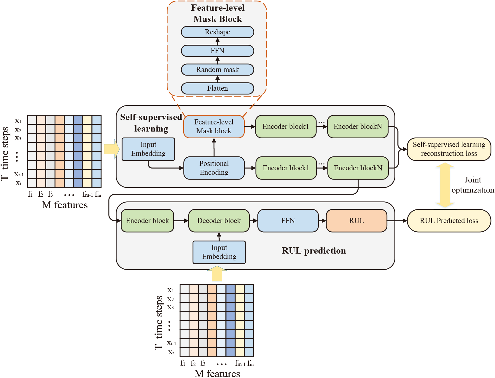

3.2 Model architecture

The proposed FMSL method adopts the encoder-decoder structure, which consists of two parts: the self-supervised learning part and the RUL prediction part. The overall architecture of the FMSL is shown in Fig. 1. The input features first undergo a self-supervised learning process. Different from the encoding process of previous methods, the input features enter two learning streams after input embedding and position encoding, respectively. One of the learning streams is stacked only by traditional Transformer encoding layers, and the other is stacked by feature-level mask blocks and traditional Transformer encoding layers. The two learning streams encode the original input features and features after feature-level masking, respectively. By comparing the latent variables encoded by the two learning streams, the encoder can learn more fine-grained feature-level information instead of simply learning fixed feature weights through labels. Then, to stabilize the model’s learning, the feature information extracted by the learning stream stacked by the traditional Transformer coding layer is input into the subsequent remaining life prediction process. When predicting RUL, the input feature information is re-encoded and entered into the decoder with the original input features together. Through the multi-head attention mechanism, the attention between the current encoded information and the final stage degraded information in the original feature is realized, and the predicted RUL is then output through a fully connected feedforward network (FFN). The FMSL method jointly optimizes the RUL prediction loss and mask reconstruction loss. We will describe the two parts of the FMSL method in detail later.

3.3 Self-supervised learning

The self-supervised learning process mainly consists of two learning streams: one is stacked by the encoder layer of the traditional Transformer to extract the original feature information, and the other is stacked by the mask block and encoder layer for feature restoration. The self-supervised learning process mainly consists of an input embedding layer, positional encoding layer, feature-level mask block, and encoder layer.

3.3.1 Input embedding layer

This layer is essentially a fully connected feedforward neural network. Raw input data can be mapped from low dimensional space to high dimensional space through this layer, increasing the nonlinearity of the model. In this paper, the original feature data will first be processed through the sliding window (see the Section 4.4.2 for details of the sliding window). We define the original feature sequence after the sliding window processing as ${{X}_{in}}\in{{\mathbb{R}}^{T\times{{D}_{\textit{input}}}}}$ , where ${{D}_{\textit{input}}}$ refers the original dimension of the input sequence, $T$ represents that there are $T$ time points within the sliding window. After passing through the input embedding layer, the original input features ${{X}_{in}}$ are mapped to ${{D}_{E}}$ dimensional vectors ${{X}_{em}}\in{{\mathbb{R}}^{T\times{{D}_{E}}}}$ .

3.3.2 Positional encoding layer

Different from the structure of RNN and LSTM, Transformer-based networks do not consider the position information of the sequence. If two-time points ${{x}_{t}}$ , ${{x}_{t+i}}$ swap positions, the output of the final model will not change. To use the positional information, we add tokens to the original feature sequence to make the model fully utilize the position information between positions. There are several commonly used positional encodings, such as learnable positional encoding [19] and trigonometric function positional encoding [20]. Among them, the learnable positional encoding is to set a randomly initialized learnable vector for each position. It can be continuously learned with the model training, and different position vectors can be assigned to different positions. The trigonometric function positional encoding also assigns different position vectors to different positions, but the trigonometric function positional encoding is an artificially set fixed vector, unlike the learnable vector. The experiments of the original Transformer show that the final effect of the model using the learnable positional encoding and the trigonometric function positional encoding is similar, so in order to reduce the model parameters, we use the trigonometric function positional encoding. The trigonometric function positional encoding formula is as follows:

$\displaystyle{{p}_{(\textit{posi},2i)}}=\sin(\textit{posi}/{{10000}^{2i/{{D}_{% Em}}}})$ (2) $\displaystyle{{p}_{(\textit{posi},2i+1)}}=\cos(\textit{posi}/{{10000}^{2i/{{D}% _{Em}}}})$ (3)

where posi refers to the position of the time series and $i$ refers to the feature dimension. The input ${{X}_{em}}$ is sent to the positional encoding layer, and then the sequence ${{X}_{\textit{posi}}}\in{{\mathbb{R}}^{T\times{{D}_{E}}}}$ encoded by the positional encoding layer will be input to the feature-level mask block and encoder layer.

Figure 2.

Flowchart of the feature-level mask. All features within a time window are pulled into one dimension by flattening, and fine-grained features are randomly masked using mask tokens. Remove the masked features and use FFN to restore them to the original dimensions. 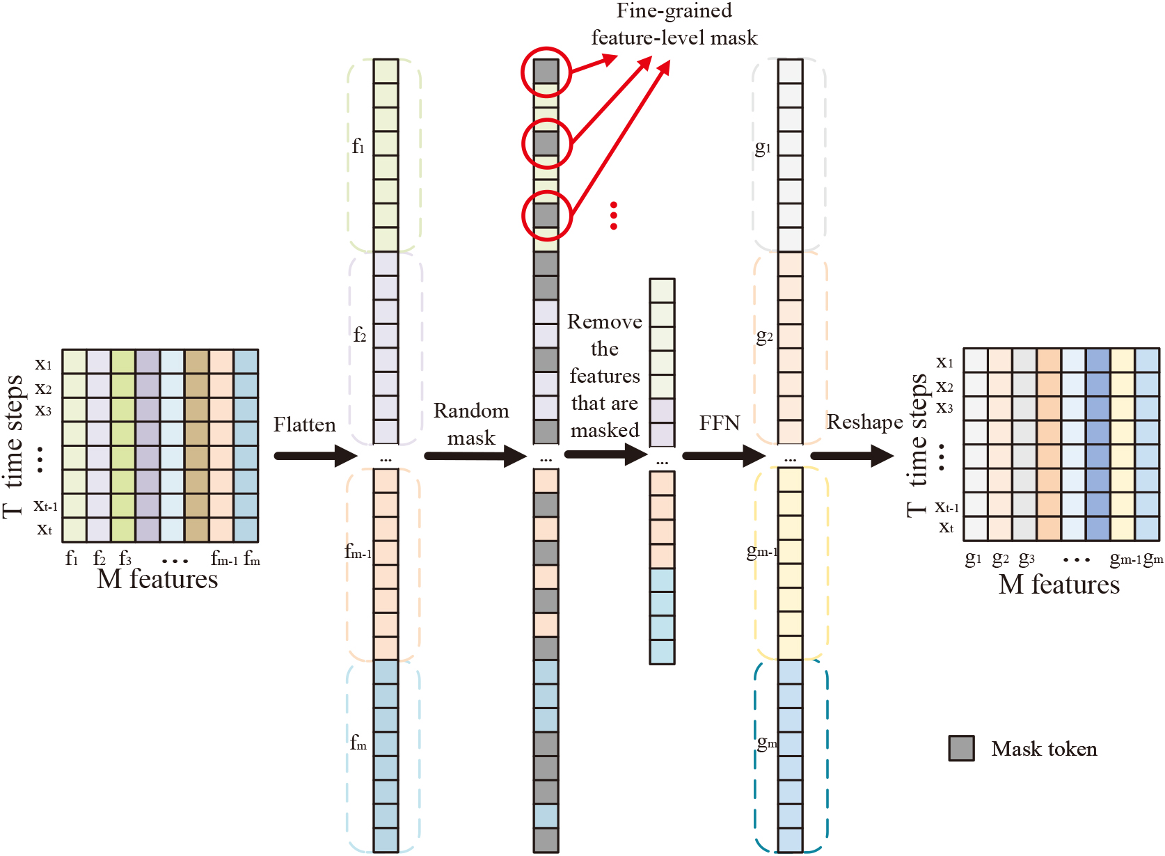${{f}_{i}}$ represents the original feature, ${{g}_{i}}$ represents the reconstruction feature, $i=(1,2,\ldots,m)$ .

3.3.3 Feature-level mask block

The importance of the same feature for degradation in different working conditions should be different, so the weights of features in different working conditions should not be uniform and constant. We propose feature-level mask blocks to enable the model to learn more precise correlations between features rather than being restricted by fixed feature weights. For the output ${{X}_{\textit{posi}}}$ after positional encoding, we will flatten the 2D matrix into a 1D sequence and then conduct sampling and deletion on the feature level of this 1D sequence. Our sampling strategy is straightforward and simple: we randomly sample from the uniform distribution to generate the index of the mask and remove the corresponding selected feature values. We call this process the “random mask.” After that, we input the 1D sequence after masking into the fully connected network layer and restore it to the original total feature number $T\times{{D}_{E}}$ through the transformation of the neural network. Re-transform it into a 2D matrix of the input feature shape ( ${{\mathbb{R}}^{T\times{{D}_{E}}}}$ ) to facilitate feature extraction and restoration in the subsequent stacked encoder layer. Figure 2 shows the flow chart of the feature-level mask block.

Figure 3.

Structure of the encoder and decoder.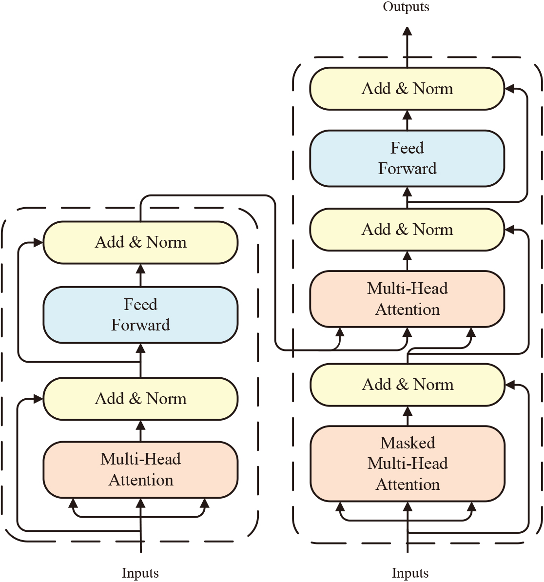

3.3.4 Encoder layer

The encoder mainly contains two network sub-layers: multi-head self-attention mechanism and FFN. The structure of the encoder layer is shown in Fig. 3. The multi-head attention mechanism is improved from the self-attention mechanism. First, three required vector matrices are obtained for the self-attention mechanism by training three neural networks: the query $Q\in{{\mathbb{R}}^{T\times{{D}_{E}}}}$ , the key $K\in{{\mathbb{R}}^{T\times{{D}_{E}}}}$ , and the value $V\in{{\mathbb{R}}^{T\times{{D}_{E}}}}$ . The dot product of the query with keys is then calculated, and a scaling factor $\sqrt{{{D}_{E}}}$ is used to obtain a stable gradient during training. Then the softmax function is used for the dot product value after scaling by a scale factor to get the attention weight of the value vector. Finally, multiply the attention weight and the value vector to obtain the final attention output, and the calculation formula is as follows:

$\displaystyle\textit{Attention}(Q,K,V)=\textit{softmax}\left(\frac{Q{{K}^{T}}}% {\sqrt{{{D}_{E}}}}\right)V$ (4)

where ${{K}^{T}}$ refers to the transpose of the matrix $K$ . $Q{{K}^{T}}$ refers to the similarity between query and key. The similarity is normalized with the softmax function to ensure that the range of similarity values does not increase with the stacking of attention. Through the above process, two time points with large similarity will be calculated with a large weight, even if they are far apart from each other. So the attention mechanism is good at capturing the correlation between long time series. The multi-head attention mechanism extracts information from different subspaces by setting multiple attention heads based on self-attention, which makes the network show better predictive performance. The calculation formula of the multi-head attention mechanism is as follows:

$\displaystyle\textit{MultiHeadAttention}(Q,K,V)=\textit{Concat}({{h}_{1}},{{h}% _{2}},\ldots,{{h}_{i}},\ldots,{{h}_{h}}){{W}^{o}}$ (5)

where the parameter matrix ${{W}^{o}}\in{{\mathbb{R}}^{h{{D}_{E}}\times{{D}_{E}}}}$ , $h$ represents the head number of the multi-head attention mechanism. ${{h}_{i}}=\textit{Attention}{{(Q,K,V)}_{i}}$ represents the self-attention result of the ith self-attention head.

The results of the multi-head attention mechanism are input to the feedforward neural network through residual connection and layer normalization. The role of residual connection is to avoid gradient vanishing as the number of model layers increases during the training process. Layer normalization is to accelerate the convergence speed and makes the model more robust.

3.4 Prediction of RUL

The input embedding layer, encoder layer, decoder layer, and feedforward neural network layer constitute the RUL prediction part. For the abstract information learned in the self-supervised learning part, the abstract information will be more conducive to reconstructing the original feature sequence because of the influence of the joint training of mask reconstruction loss. If the information is directly used for the RUL prediction, the results may be unsatisfactory because the extracted abstract information focuses too much on reconstructing the original feature sequences. So we will extract the information once again after the encoder layer. Then, the important degradation information extracted by the decoder is considered so that the abstract information input into the feedforward neural network contains more degradation information related to the RUL. After that, it is mapped through a feedforward neural network to get the final RUL value.

The main structure of the decoder layer which mainly consists of a masked multi-head attention mechanism and encoder-decoder attention mechanism is shown in Fig. 3. For RUL prediction, we believe that among all the time points in the time window of the original feature, the time points closer to the time point of the final RUL prediction contain more important degradation trends information. Therefore, we use the masked multi-head attention mechanism to mask out the earlier time points in the time window, making sure that the model can notice more important point-wise information which is more relevant to degradation. At the encoder-decoder attention mechanism, the query comes from the output after residual layer connection and layer normalization, and the keys and values come from the encoder output. The information of the encoder output can then be extracted, which can focus on important degradations in the decoder to predict the RUL more accurately.

3.5 Joint optimization

3.5.1 Reconstruction loss

The self-supervised learning method of feature mask reconstruction is used to enable the model to pay more attention to the fine-grained correlation between features. For a given input window sample ${X}^{i}_{in}\in{{\mathbb{R}}^{T\times M}}$ , we put this data through two learning streams respectively to obtain the output ${X}^{i}_{\textit{mask-out}}$ and ${X}^{i}_{\textit{out}}$ . We define the Mean Square Error (MSE) between the two outputs of self-supervised learning as the reconstruction loss. The calculation formula of the reconstruction loss is as follows:

$\displaystyle{{L}_{\textit{rec}}}=\frac{1}{N}\sum\limits_{i=1}^{N}\left\|{X}^{% i}_{\textit{mask-out}}-{X}^{i}_{\textit{out}}\right\|^{2}$ (6)

where ${{L}_{\textit{rec}}}$ refers to the loss of reconstruction, and $N$ refers to the total samples number.

3.5.2 Predicted loss of RUL

The MSE between the predicted RUL value and the actual RUL label value of each input window sample is defined as the RUL prediction loss. The calculation formula of the prediction loss is as follows:

$\displaystyle{{L}_{\textit{rul}}}=\frac{1}{N}\sum\limits_{i=1}^{N}{\left\|% \textit{RUL}_{\textit{pre}}^{i}-\textit{RUL}^{i}\right\|^{2}}$ (7)

where ${{L}_{\textit{rul}}}$ refers to the predicted loss of RUL, $\textit{RUL}_{\textit{pre}}^{i}$ refers to the predicted RUL value and $\textit{RUL}^{i}$ represents the real RUL label value.

3.5.3 Joint loss

The FMSL aims to simultaneously optimize the feature-level mask reconstruction loss and RUL prediction loss. Joint optimization of these two losses can make the model learn more fine-grained correlations between features and can also provide more abstract potential representations to improve the accuracy of RUL prediction. The joint loss can be expressed by the following formula:

$\displaystyle L=(1-\alpha){{L}_{\textit{rec}}}+\alpha{{L}_{\textit{rul}}}$ (8)

where $L$ represents the joint loss used for training and $\alpha$ is a parameter that can control the proportion of mask reconstruction loss and RUL prediction loss. The parameter values and the influence of different parameters on the experimental results will be analyzed in detail in subsequent experiments.

4. Experiment

We will detail the experimental datasets, evaluation metrics, parameter settings, and experimental results in this section. The performance of FMSL is evaluated through experiments and compared with state-of-the-art RUL prediction methods to verify the advantages of FMSL. All experiments were performed on a workstation equipped with Intel(R) Core(TM) I9-10900x 10-core 3.70GHz CPU and NVIDIA GeForce RTX 3090 GPU. The code is written using PyTorch, and the network training and testing are completed on the GPU.

4.1 Benchmark dataset

In this paper, we evaluate our method using the widely used C-MAPSS dataset, which is generated by a thermo-dynamical simulation model to simulate damage propagation and performance degradation [22, 29]. To enhance the authenticity of the data, random measurement noise is added to the sensor simulation output to simulate the noise fluctuation of real data. The layout diagram of the engine simulation is illustrated in Fig. 4, and it includes low and high-pressure compressors, a combustor section, and low and high-pressure turbines. By adjusting the settings, we can simulate various operating conditions for the engine, such as altitudes ranging from sea level to 40,000 ft (12,192 m), Mach numbers from 0 to 0.90, and sea-level temperatures ranging from $-$ 60 to 103 ${}^{\circ}$ F ( $-$ 51 to 39 ${}^{\circ}$ C). The C-MAPSS dataset contains four different sub-datasets collected under different working conditions. The FD001 dataset simulates data in one operating condition and one failure mode; the FD002 dataset simulates data in six operating conditions and one failure mode; the FD003 dataset simulates data in one operating condition and two failure modes; the FD004 dataset simulates data in six operating conditions and two failure modes. Each subset provides a training set and a test set. The data of the training set includes the entire life cycle of the engine running from a certain point to the end of life. The test set only contains sensor measurement data recorded for a specific operating cycle of a specific number of engines. It is unknown whether it is a normal operating or degraded cycle. Our goal is to train the model using the sensor measurements recorded in the given training set to make RUL predictions for each engine in the test set. The data provided by C-MAPSS includes measurements from 21 different sensors, but not all of the sensors can provide useful degradation information. Sensor 1, 5, 6, 10, 16, 18, and 19 always keeps constant. Therefore, we used the remaining 14 sensors after deleting these sensors for RUL prediction. In addition, previous studies have shown that the mean value and regression coefficient estimation of time series data can provide useful information [14], which is helpful for RUL prediction. Therefore, we add this feature information to the feature sequence. Table 1 shows the details of the C-MAPSS dataset.

Table 1
Details of the C-MAPSS data set

Subsets	FD001	FD002	FD003	FD004
Training number of engines	100	260	100	249
Testing number of engines	100	259	100	248
Fault modes	1	6	1	6
Operation conditions	1	1	2	2
Training samples	17731	35819	21820	41578
Testing samples	100	259	100	248

Figure 4.

Layout diagram of the engine simulation [29].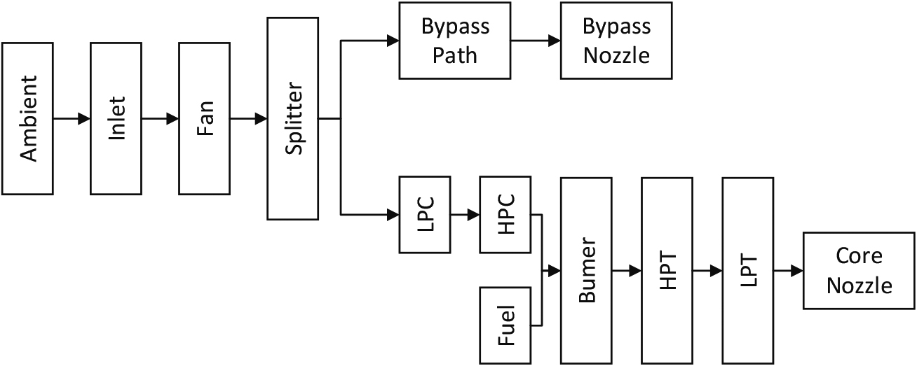

4.2 Evaluation metrics

In this experiment, we use the root mean square error (RMSE) and score metric to verify the performance of our proposed method. Assuming that the $N$ is the number of samples, ${{y}_{i}},\widehat{{{y}_{i}}}$ is the ith real RUL label and the ith predicted RUL, respectively. The root mean square error can be calculated as follows:

$\displaystyle\textit{RMSE}=\sqrt{\frac{1}{N}\sum\limits_{i=1}^{N}{{{(\widehat{% {{y}_{i}}}-{{y}_{i}})}^{2}}}}$ (9)

RMSE treats the larger predicted value as the same as the smaller predicted value. However, for actual PHM tasks, compared with the predicted RUL which is greater than the actual RUL, we prefer the predicted RUL, which is less than the actual RUL. Therefore, the score metric was proposed in the 2008 Prognostic and Health Management (PHM) Data Challenge [29]. The score metric gives more penalty to delayed prediction, and its specific formula is as follows:

$\displaystyle\textit{Score}=\left\{\begin{array}[]{ll}\sum_{{i=1}}^{N}{\left({% {e}^{-\frac{\widehat{{{y}_{i}}}-{{y}_{i}}}{13}}}-1\right),}&\widehat{{{y}_{i}}% }\leqslant{{y}_{i}}\\ \sum_{i=1}^{N}{\left({{e}^{\frac{\widehat{{{y}_{i}}}-{{y}_{i}}}{10}}}-1\right)% ,}&\widehat{{{y}_{i}}}>{{y}_{i}}\\ \end{array}\right.$ (10)

4.3 Parameter settings

The Adam optimizer is used during training to optimize the model. In addition, 5% of the data in each original data subset is divided into verification sets. And the early stop strategy is applied to avoid overfitting. When the verification loss in 15 consecutive cycles is greater than the minimum verification loss recorded in history, the training process is stopped in advance. The optimal training result is obtained with the network parameter that has the minimum verification loss. During the self-supervised learning process, the number of stacked encoders for both learning streams is 4. The stacked encoder and decoder modules are 2 and 1 during the RUL prediction process. We set the epoch to 100 for FD001 and FD003 datasets and 200 for FD002 and FD004 datasets. The batch size is set to 256, and the learning rate is set to 0.001. We carried out special experiments for parameter selection and analysis to get the best model parameters. The influence of parameters on the predicted results will be discussed later.

4.4 Data preprocessing

4.4.1 Regularization

Data collected by different sensors have different units and scales, which will affect the accuracy of RUL prediction [30] and make it difficult for the neural network to converge. Min-max normalization is used to limit the value of each sensor to [0, 1] and transform the data with different units to dimensionless data. The specific formula of min-max normalization for data ${{X}_{i}}\in{{\mathbb{R}}^{m}}$ (where $m$ represents the number of features) is as follows:

$\displaystyle\widetilde{{{X}_{i}}}=\frac{{{X}_{i}}-\min({{X}_{i}})}{\max({{X}_% {i}})-\min({{X}_{i}})}$ (11)

where $\widetilde{{{X}_{i}}}$ represents regularized ${{X}_{i}}$ , $\min({{X}_{i}})$ represents the minimum value in ${{X}_{i}}$ , $\max({{X}_{i}})$ represents the maximum value in ${{X}_{i}}$ . Figure 5 shows the regularized data.

Figure 5.

Regularized data of engine 10 in the FD001 dataset.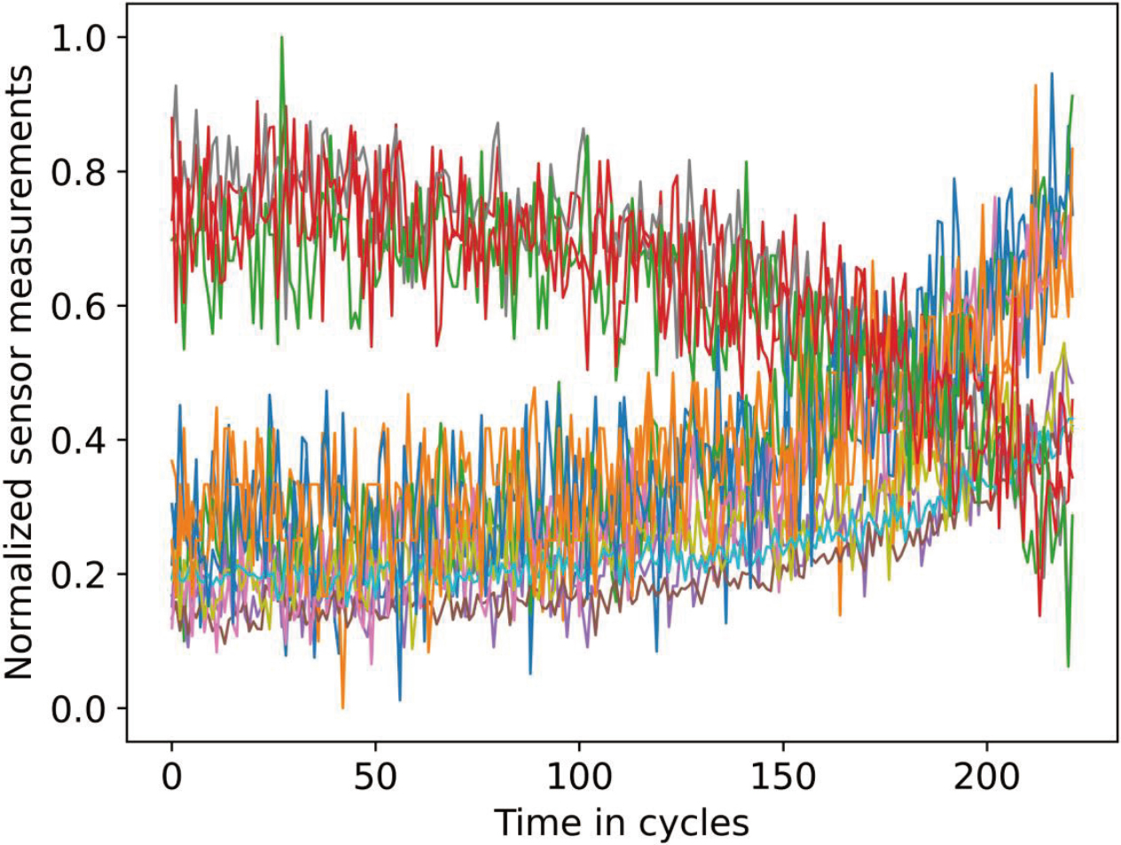

4.4.2 Sliding window and RUL label

The sliding window is used to process the original feature data to obtain the windowed samples. Figure 6 shows an example of sliding window processing and RUL labels. A longer time window contains more valuable information, which helps improve predictive performance [31]. However, a long time window may make the model more complex and affect its applicability [22]. Therefore, we will conduct experiments to discuss the influence of time window size on the model’s prediction performance and select the appropriate window size (see Section 4.5.3 for experiment details). $W$ in Fig. 6 is the size of the time window, and each sliding step is set to 1. The interval from the last time point in the time window to the failure point is the RUL of this time point. The RUL of this point is labeled as the RUL label of the entire window. The figure shows two sliding windows ( ${{T}_{0}}\sim{{T}_{W}}$ and ${{T}_{n}}\sim{{T}_{W+n}}$ ) and their corresponding RUL labels.

Figure 6.

Sliding windows and their corresponding RUL labels.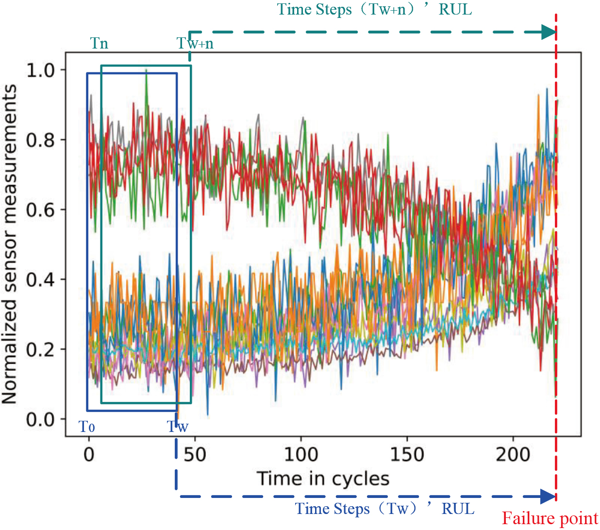

4.4.3 Piece-wise RUL

An important problem for RUL prediction is obtaining usable RUL labels from the data when given continuous complete life cycle data from normal operation to failure. Some scholars assume that the degeneration of the components varies linearly with time. However, system degradation can be ignored in the early stage of the whole life cycle in practice. For learning models, if the RUL label changes linearly with time, it will mislead the model and further affect the prediction results of the model. Therefore, piece-wise is used to represent the real remaining life, as shown in Fig. 7. It assumes that RUL remains unchanged at the beginning of the operation. When the system reaches the degradation point, RUL decreases linearly with time. Following previous studies [6, 17, 30], we use a constant ${\textit{RUL}_{\max}}$ to represent the initial RUL and set it to 125.

Figure 7.

Piece-wise RUL and actual RUL.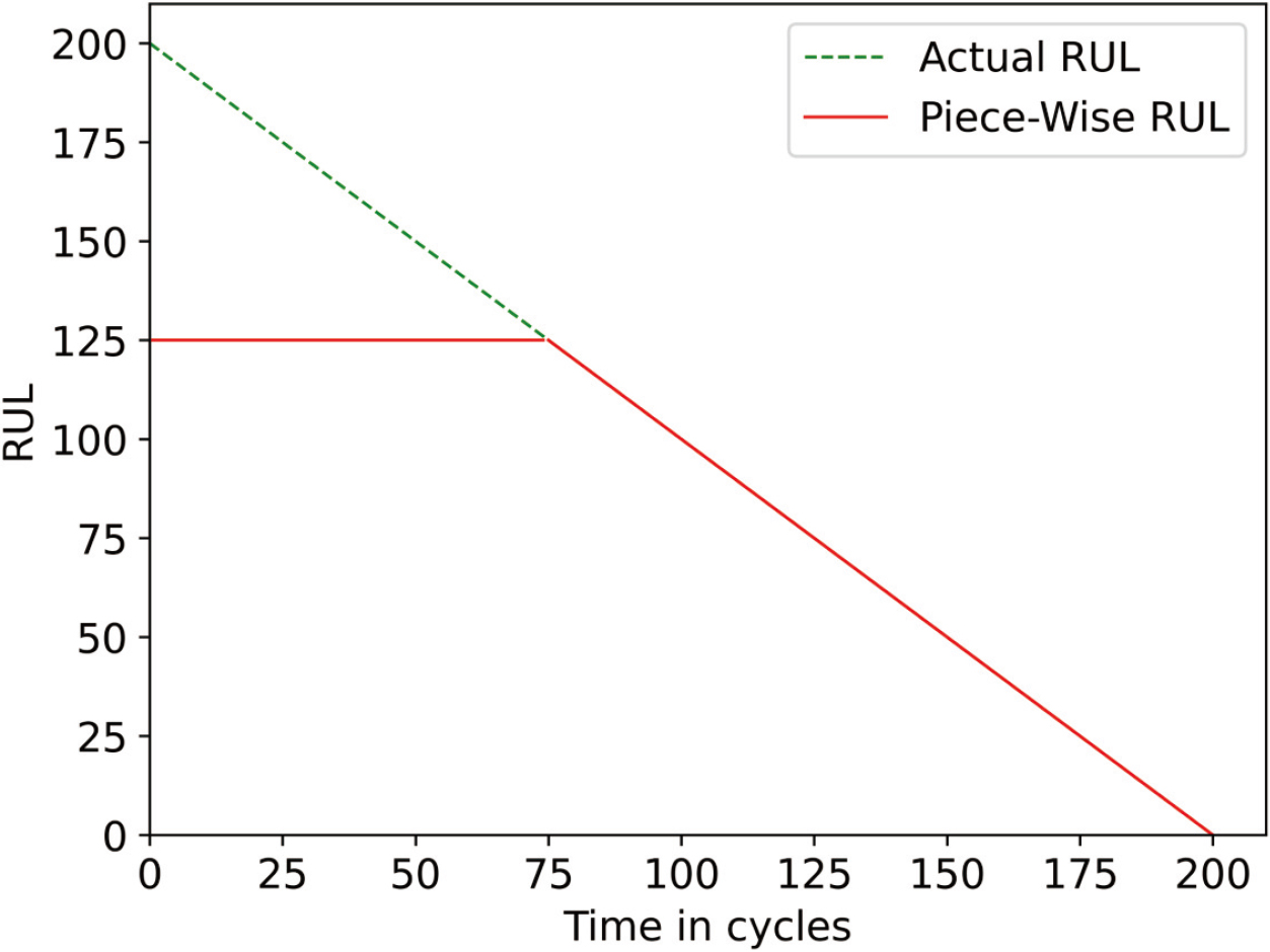

4.5 Experimental analysis

In this part, we compare the proposed method with other SOTA methods to verify the performance of the FMSL. We also performed ablation experiments to evaluate the effect of the feature-level mask reconstruction task. In addition, the influence of the mask rate and other parameters on the method will also be discussed.

4.5.1 Comparison with other methods

We compare the FMSL method with some machine learning and other state-of-the-art deep learning RUL prediction methods to verify the performance of the FMSL method. These methods include four categories: methods based on machine learning [32], methods based on RNN/CNN [24, 25, 26], methods combined with attention mechanism [3, 27, 28], and methods based on Transformer [17, 22]. In order to reduce the randomness of the results, our results are averaged after repeating the prediction ten times. Table 2 shows the RUL prediction performance of the FMSL method and other SOTA methods. The bold results indicate the best performance.

Table 2
Performance comparison of the proposed method and state-of-the-art methods

Methods	FD001	FD002	FD003	FD004	Average	FD001	FD002	FD003	FD004	Average
	RMSE					Score
LR	20.82	21.71	21.77	30.74	23.76	1251.32	2797.95	2731.29	15466.85	5561.85
GBRT	17.41	17.55	21.08	19.82	18.97	1107.41	2716.1	2896.36	3253.24	2493.28
SVR	20.96	41.99	21.05	45.35	32.34	1381	589900	1598	371140	241004.75
BiLSTM	13.65	23.18	13.74	24.86	18.85	295	4130	317	5430	2543.00
DCNN	12.61	22.36	12.64	23.31	17.73	273.7	10412	284.1	12466	5858.95
KONG	16.13	20.46	17.12	23.26	19.24	303	3440	1420	4630	2448.25
DATCN	11.78	16.95	11.56	18.23	14.63	229.48	1842.38	257.11	2317.32	1161.57
DARNN	12.04	19.24	10.18	18.02	14.87	261.95	933.58	247.85	2587.44	1007.71
AGCNN	12.42	19.43	13.39	21.5	16.69	225.51	1492	227.09	3392	1334.15
DAST	11.43	15.25	11.32	18.36	14.09	203.15	924.96	154.92	1490.72	693.44
DAA	12.25	17.08	13.39	19.86	15.65	198	1575	290	1741	951.00
FMSL	12.32	12.74	12.32	17.14	13.63	266.36	625.63	306.04	1348.92	636.74

Table 1 shows that FD001 and FD003 are the data of one or two kinds of faults collected under one working condition, respectively. In comparison, FD002 and FD004 are the data of one or two kinds of faults collected under six working conditions, respectively. Therefore, the prediction difficulties of the data subsets FD001 and FD003 are less than that of FD002 and FD004, which can also be clearly reflected in the experimental results: The RMSE and score of the FD001 data subset are 12.32 and 266.36, respectively, while those of the FD004 data subset is 17.14 and 1348.92, respectively. Although FD002 and FD004 are data collected under six working conditions, FD002 contains only one fault type, and FD004 contains two fault types. So the RMSE and score of FD004 are also larger than those of FD002, indicating that FD004 is harder to predict RUL. In addition, as shown in Fig. 8, we plot the visualized results of predicted RUL using the FMSL method and actual RUL for all engines in four test data subsets. In order to facilitate observation and analysis, the engine units are sorted by actual RUL value from largest to smallest. The $X$ axis represents the number of the engine unit, and the $Y$ axis represents the number of RUL cycles. As can be seen from Fig. 8, models can accurately predict whether the engine is in normal working condition or in the process of degradation (the actual RUL is less than the maximum RUL 125). Moreover, we find that when the real RUL of the engine is small, the RUL predicted by the model is significantly more accurate. This is because the engine gradually changes from normal operation to degradation and failure with the use of the engine. A smaller true RUL of the engine indicates that the engine has degraded for a longer time and is closer to failure. The data collected during this process contains more degradation information, and the degradation characteristics become more and more obvious. Therefore, the proposed method can extract more degradation information from the sensor data to better predict the engine’s RUL.

Figure 8.

Visualization results of RUL prediction (a) FD001 test data subset (b) FD002 test data subset (c) FD003 test data subset (d) FD004 test data subset.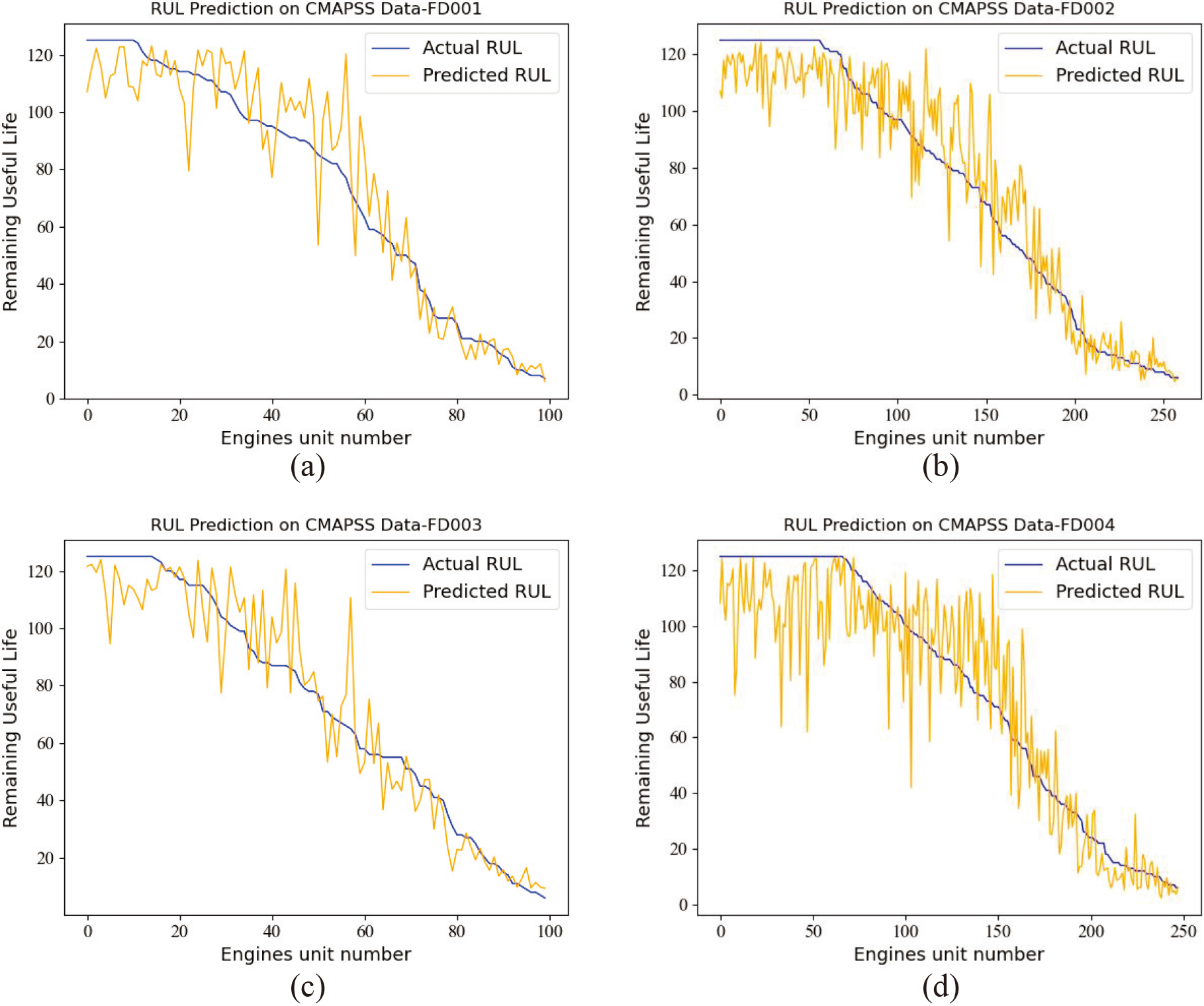

In addition, we also compared our method with other methods. It can be seen from Table 2 that the RMSE and score of our proposed method on the FD002 data subset are 12.74 and 625.63, and the RMSE and score on the FD004 data subset are 17.14 and 1348.92. Compared with other methods, our results have a great improvement. For example, in the FD002 data set, the proposed method improves by 16% and 32% in RMSE and score, respectively, compared with the second-ranking method. This is because our method uses a self-supervised learning method of feature mask and reconstruction. Through the joint learning of the masking reconstruction task and the RUL prediction task, the model learns more fine-grained correlations and dependencies of different features at different times. This will make our model more generalized when dealing with data collected under complex working conditions such as FD002 and FD004, and the experimental results have well confirmed our ideas. It can be seen from the table that although the proposed method does not achieve the best results on FD001 and FD003 datasets, it also achieves competitive results. The proposed method performs slightly worse on the above two datasets than some methods that consider the serial correlation as a whole. When the data is collected under a single working condition, an overall mapping relationship can be used to obtain better results. However, such an overall mapping will have the negative effect of confusion under multiple operating conditions, leading to the erroneous mapping between the degradation information of different operating conditions and the RUL. The poor performance of these methods on the FD002 and FD004 datasets in the table can also reflect this reason. In reality, a large amount of collected sensor data is often obtained under various working conditions, so the situation of multiple working conditions should be considered more seriously. The proposed method achieves the best average results on the two evaluation metrics of the four datasets, considering the multi-condition problem. Based on the above results and discussion, the FMSL model proposed in this paper has better modeling ability and powerful information extraction ability for complex multi-dimensional time series data and has a better application prospect in practical RUL prediction.

4.5.2 Ablation study of FMSL

In this work, we propose a feature-level mask reconstruction self-supervised learning method. The model can learn a more stable correlation between features by designing specifically for fine-grained features. This enables the model to achieve better prediction performance in complex situations such as multiple operating conditions. To evaluate the effectiveness of the feature-level mask, we conduct ablation experiments. In the experiment, we carried out the experiment of our proposed method and the experiment of removing the feature-level mask block, respectively. The model without the feature-level mask block is equivalent to an original Transformer model with an asymmetric encoding and decoding structure, and the model adopts the same number of encoding and decoding layers as our proposed method. We conducted experiments on all four data subsets, and the experimental results are shown in Table 3. It can be seen from the experimental results that compared with the original Transformer model, our proposed method has a large improvement on all data subsets. It also shows that the proposed joint optimization of the feature-level mask block and the corresponding reconstruction loss can enable the model to learn overall information between features that is applicable under different working conditions, resulting in better prediction performance and generalization performance of the model.

Table 3
Ablation study of the proposed architecture

Method	Metric	FD001	FD002	FD003	FD004
FMSL w/o feature-leavel mask	RMSE	12.76	13.78	12.79	17.26
	Score	287.69	666.39	412.44	1435.94
FMSL	RMSE	12.32	12.74	12.32	17.14
	Score	266.36	625.63	306.04	1348.92

4.5.3 Parameter analysis

There are three important parameters in the proposed method: the length of the sliding window, the masking rate of the feature-level mask block, and the proportion of prediction loss in the joint loss ( $\alpha$ in the formula $L=(1-\alpha){{L}_{\textit{rec}}}+\alpha{{L}_{\textit{rul}}}$ ).

It is necessary to set an optimal sliding time window size [21]. A small sliding time window may lack sufficient degradation information, while a large sliding time window will enlarge the size of the model and increase the complexity of training and prediction. Therefore, setting an appropriate sliding time window will improve the prediction accuracy. In order to select the optimal sliding window length and not to make the sliding window too large or too small, we test the model performance with different sliding time window sizes from 20 to 80 for each subset of data at ten intervals. The experimental results are shown in Fig. 9. From the figure, we can find that FD001 and FD002 have relatively simple data and a fast degradation process, and the long-term window may include both normal operation and degradation time, which will interfere with the prediction. Therefore, a small-length sliding time window achieves better experiment results. However, when processing the data collected under complex conditions such as FD003 and FD004, the prediction effect of a small sliding window is poor because it contains less degradation information. Therefore, considering the two results of RMSE and Score for different data subsets, we choose the sliding window length of the FD001 data subset to be 30. The sliding window length of the FD002 data subset is 70. The sliding window length of the FD003 data subset is 30. The sliding window length of the FD004 data subset is 80.

Figure 9.

Influence of different sliding window lengths on model performance (a) Performance of different sliding window lengths on different data subsets (RMSE) (b) Performance of different sliding window lengths on different data subsets (Score).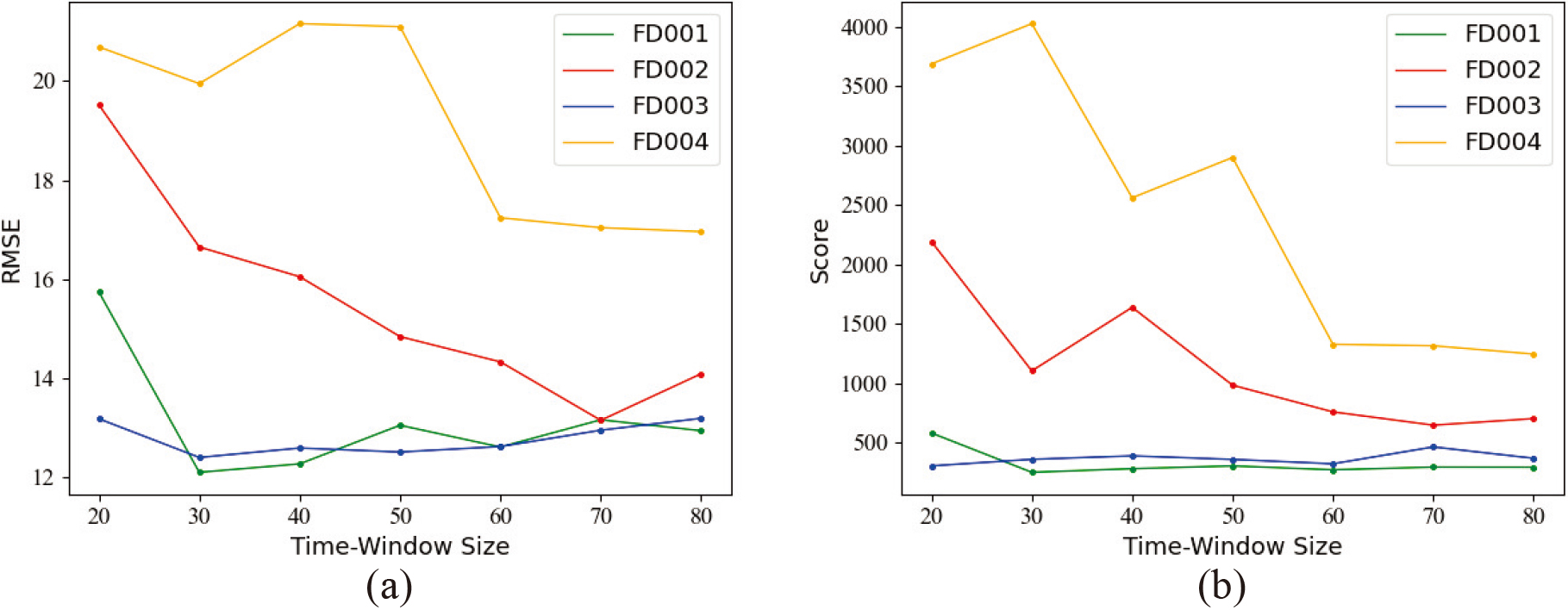

The mask rate of the feature-level mask block refers to the random mask rate of the original feature data in the self-supervised learning process. We take the most complex FD004 data subset as an example to test the model’s predictive performance at different mask rate settings with an interval of 0.1. Experiment results are shown in Fig. 10a. Different masking rates affect the information loss and feature learning ability of the model. We aim to achieve a balance between information loss and model learning ability by adjusting the masking rate to achieve optimal prediction results.When the masking rate is 0.1, the information loss is minimal and the model achieves good results. As the masking rate increases, information loss becomes greater while the model’s learning ability becomes stronger, leading to the prediction results first getting worse and then getting better. However, when the masking rate is greater than 0.4, the model’s RUL prediction performance gradually deteriorates as the masking rate increases. This may be due to the masking rate being too high, resulting in a limited amount of original information available for the model to utilize and leading to a significant loss of useful information and reduced prediction performance. At a masking rate of 0.2, our proposed method has the worst results on the FD004 data subset. Nevertheless, it still outperforms the results of the ablation experiments without the introduction of the self-supervised learning task, indicating the usefulness of our self-supervised task for prediction. Another important parameter is the percentage of prediction loss in the joint loss. By tuning this hyperparameter, we can adjust the proportion of reconstruction loss and prediction loss in the overall loss. We also take the FD004 data subset as an example and test the model’s predictive performance at different proportion of the predicted loss in the overall loss with an interval of 0.1. Experiment results are shown in Fig. 10b. The abscissa in the figure represents the proportion of the predicted loss in the overall loss. The figure shows that the prediction performance of the model decreases as the proportion of predicted loss to total loss increases. This indicates that paying more attention to self-supervised learning in model training can significantly improve prediction accuracy. And it also reflects from the side that the feature-level mask block can enable the model to learn more representative information between features. Through joint learning of the self-supervised learning task and prediction task, the model can learn a more robust representation that is advantageous for the RUL prediction task.

Figure 10.

Influence of different masking rates and proportions of prediction loss in the joint loss on model performance (a) Performance of FD004 data subsets at different masking rates (b) Performance of FD004 data subsets at different proportions of prediction loss in the joint loss.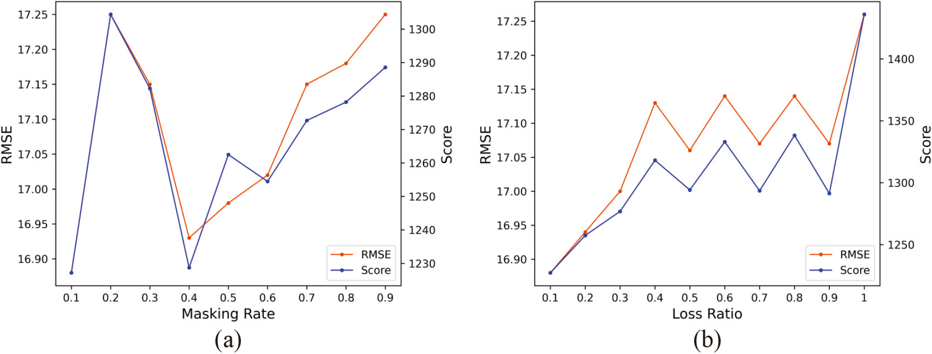

5. Discussion

This paper introduces self-supervised learning in RUL prediction, achieving optimal average performance with a well-designed model. Traditional RUL prediction methods utilize attention mechanisms to calculate the correlation between the entire sequence or features, neglecting the finer-grained point-wise information. This leads to the loss of useful information for RUL prediction. In addition, data are usually collected under various working conditions, and the importance of different features may change during the system’s degradation. Traditional attention-based methods may not capture this change since they do not consider the dependency of different features at different times, thereby affecting RUL prediction accuracy.

Self-supervised learning has recently gained attention in extracting representations from unlabeled data for downstream tasks [33]. By incorporating a self-supervised task of feature-level mask reconstruction, the model is encouraged to consider feature-level correlation from a finer-grained perspective. Reconstructing the entire original sample using feature points that are not masked enables the model to learn the dependency and the changes of correlation between different features at different times. By learning the mask reconstruction task and the RUL prediction task jointly, the model can extract point-wise and overall trend information simultaneously, enabling it to better model complex time series and improve RUL prediction accuracy.

Although the proposed method significantly improves the prediction performance on complex datasets with multiple working conditions and obtains the optimal average performance, it does not achieve the best results on all datasets. This may be caused by the overfitting problem under simple working conditions, which requires further investigation and improvement in future research.

6. Conclusion

The FMSL in this paper is different from the traditional deep learning method that only considers the correlation between the entire sequences. We have specially designed the model to learn the correlation between the feature values. The proposed feature-level mask block makes the model pay more attention to point-wise information. Through the joint learning of the masking reconstruction task and the RUL prediction task, the model learns more fine-grained correlations and dependencies of different features at different times. In this way, the model’s generalization performance is enhanced, so the model has better performance under complex working conditions. It alleviates the problem that the coarse-grained feature extraction limits the model’s learning performance and generalization performance, which is commonly found in previous studies.

In practical situations, collecting massive amounts of data under multiple operating conditions is common. The proposed method has better practicability and wider application prospects. We conduct ablation experiments and compare the FMSL method with other SOTA methods. The experimental results demonstrate the effectiveness of feature-level mask reconstruction self-supervised task and the superiority of FMSL. In the future, we will focus on the potential of attention methods and mask reconstruction methods in terms of model interpretability. An important research direction in the future is to improve the interpretability of the depth prediction model.

Footnotes

Acknowledgments

The author would like to thank the colleagues of the deep learning group who participated in this discussion.

References

Yuan

Dong

Lin

Liu

, Remaining useful life estimation of engineered systems using vanilla LSTM neural networks, Neurocomputing 275 (2018), 167–179. doi: 10.1016/j.neucom.2017.05.063.

Ragab

Chen

Kwoh

C.-K.

Yan

, Attention-based sequence to sequence model for machine remaining useful life prediction, Neurocomputing 466 (2021), 58–68. doi: 10.1016/j.neucom.2021.09.022.

Liu

Jia

Lin

, Remaining useful life prediction using a novel feature-attention-based end-to-end approach, IEEE Transactions on Industrial Informatics 17(2) (2021), 1197–1207. doi: 10.1109/TII.2020.2983760.

Liu

Jia

Zhang

Tan

, A multi-head neural network with unsymmetrical constraints for remaining useful life prediction, Advanced Engineering Informatics 50 (2021), 101396. doi: 10.1016/j.aei.2021.101396.

Park

J.M.

Youn

B.D.

Choi

J.-H.

Kim

N.H.

, Model-based fault diagnosis of a planetary gear: A novel approach using transmission error, IEEE Transactions on Reliability 65(4) (2016), 1830–1841. doi: 10.1109/TR.2016.2590997.

Huang

, Remaining useful life estimation via transformer encoder enhanced by a gated convolutional unit, Journal of Intelligent Manufacturing 32(7) (2021), 1997–2006. doi: 10.1007/s10845-021-01750-x.

Liu

Cheng

Wang

Long

, A method for remaining useful life prediction of crystal oscillators using the Bayesian approach and extreme learning machine under uncertainty, Neurocomputing 305 (2018), 27–38. doi: 10.1016/j.neucom.2018.04.043.

Ali

J.B.

Chebel-Morello

Saidi

Malinowski

Fnaiech

, Accurate bearing remaining useful life prediction based on Weibull distribution and artificial neural network, Mechanical Systems and Signal Processing 56 (2015), 150–172. doi: 10.1016/j.ymssp.2014.10.014.

Zhu

Liu

, Online tool wear monitoring via hidden semi-markov model with dependent durations, IEEE Transactions on Industrial Informatics 14(1) (2018), 69–78. doi: 10.1109/TII.2017.2723943.

10.

Loutas

T.H.

Roulias

Georgoulas

, Remaining useful life estimation in rolling bearings utilizing data-driven probabilistic e-support vectors regression, IEEE Transactions on Reliability 62(4) (2013), 821–832. doi: 10.1109/TR.2013.2285318.

11.

Pan

Chen

, A multi-head attention network with adaptive meta-transfer learning for RUL prediction of rocket engines, Reliability Engineering & System Safety, 2022, 108610. doi: 10.1016/j.ress.2022.108610.

12.

Liu

Zhou

Zheng

Jiang

Zhang

, Fault diagnosis of rolling bearings with recurrent neural network-based autoencoders, ISA Transactions 77 (2018), 167–178. doi: 10.1016/j.isatra.2018.04.005.

13.

J.-Y.

Chen

X.-L.

Yan

, Degradation-aware remaining useful life prediction with LSTM autoencoder, IEEE Transactions on Instrumentation and Measurement 70 (2021), 1–10. doi: 10.1109/TIM.2021.3055788.

14.

Chen

Zhao

Guretno

Yan

, Machine remaining useful life prediction via an attention-based deep learning approach, IEEE Transactions on Industrial Electronics 68(3) (2021), 2521–2531. doi: 10.1109/TIE.2020.2972443.

15.

Miao

Sun

Liu

, Joint learning of degradation assessment and RUL prediction for aeroengines via dual-task deep LSTM networks, IEEE Transactions on Industrial Informatics 15(9) (2019), 5023–5032. doi: 10.1109/TII.2019.2900295.

16.

Song

Peng

Liu

, Lithium-ion battery remaining useful life prediction based on GRU-RNN, in: 2018 12th International Conference on Reliability, Maintainability, and Safety (ICRMS), IEEE, 2018, pp. 317–322. doi: 10.1109/ICRMS.2018.00067.

17.

Zhang

Song

, Dual-aspect self-attention based on transformer for remaining useful life prediction, IEEE Transactions on Instrumentation and Measurement 71 (2022), 1–11. doi: 10.1109/tim.2022.3160561.

18.

Chen

Xie

Dollár

Girshick

, Masked autoencoders are scalable vision learners, in: Proceedings of the IEEE/CVF Conference on Computer Vision and Pattern Recognition, 2022, pp. 16000–16009. doi: 10.48550/arXiv.2111.06377.

19.

Devlin

Chang

M.-W.

Lee

Toutanova

, Bert: Pre-training of deep bidirectional transformers for language understanding, arXiv preprint arXiv:1810.04805, 2018. doi: 10.48550/arXiv.1810.04805.

20.

Vaswani

Shazeer

Parmar

Uszkoreit

Jones

Gomez

A.N.

Kaiser

Ł.

Polosukhin

, Attention is all you need, Advances in Neural Information Processing Systems 30 (2017). doi: 10.48550/arXiv.1706.03762.

21.

Ren

Liu

Huang

Yang

, MCTAN: A Novel Multichannel Temporal Attention-Based Network for Industrial Health Indicator Prediction, IEEE Transactions on Neural Networks and Learning Systems, 2022, 1–12. doi: 10.1109/TNNLS.2021.3136768.

22.

Liu

Song

Zhou

, Aircraft engine remaining useful life estimation via a double attention-based data-driven architecture, Reliability Engineering & System Safety 221 (2022), 108330. doi: 10.1016/j.ress.2022.108330.

23.

Qin

Cai

Gao

Zhang

Cheng

Chen

, Remaining Useful Life Prediction Using Temporal Deep Degradation Network for Complex Machinery with Attention-based Feature Extraction, arXiv preprint arXiv:2202.10916, 2022. doi: 10.48550/arXiv.2202.10916.

24.

Wang

Wen

Yang

Liu

, Remaining useful life estimation in prognostics using deep bidirectional lstm neural network, in: 2018 Prognostics and System Health Management Conference (PHM-Chongqing), IEEE, 2018, pp. 1037–1042. doi: 10.1109/PHM-Chongqing.2018.00184.

25.

Ding

Sun

J.-Q.

, Remaining useful life estimation in prognostics using deep convolution neural networks, Reliability Engineering & System Safety 172 (2018), 1–11. doi: 10.1016/j.ress.2017.11.021.

26.

Kong

Cui

Xia

, Convolution and long short-term memory hybrid deep neural networks for remaining useful life prognostics, Applied Sciences 9(19) (2019), 4156. doi: 10.3390/app9194156.

27.

Song

Gao

Jia

Pang

, Distributed attention-based temporal convolutional network for remaining useful life prediction, IEEE Internet of Things Journal 8(12) (2020), 9594–9602. doi: 10.1109/JIOT.2020.3004452.

28.

Zeng

Jiang

Song

, A deep attention residual neural network-based remaining useful life prediction of machinery, Measurement 181 (2021), 109642. doi: 10.1016/j.measurement.2021.109642.

29.

Saxena

Goebel

Simon

Eklund

, Damage propagation modeling for aircraft engine run-to-failure simulation, in: 2008 International Conference on Prognostics and Health Management, IEEE, 2008, pp. 1–9. doi: 10.1109/PHM.2008.4711414.

30.

Zhao

Zhang

Zio

, Remaining useful life prediction using multi-scale deep convolutional neural network, Applied Soft Computing 89 (2020), 106113. doi: 10.1016/j.asoc.2020.106113.

31.

Huang

C.-G.

Huang

H.-Z.

Y.-F.

, A bidirectional LSTM prognostics method under multiple operational conditions, IEEE Transactions on Industrial Electronics 66(11) (2019), 8792–8802. doi: 10.1109/TIE.2019.2891463.

32.

Sateesh Babu

Zhao

X.-L.

, Deep convolutional neural network based regression approach for estimation of remaining useful life, in: Database Systems for Advanced Applications: 21st International Conference, DASFAA 2016, Dallas, TX, USA, April 16–19, 2016, Proceedings, Part I 21, Springer, 2016, pp. 214–228.

33.

Eldele

Ragab

Chen

Kwoh

C.K.

Guan

, Time-Series Representation Learning via Temporal and Contextual Contrasting, in: Proceedings of the Thirtieth International Joint Conference on Artificial Intelligence, IJCAI-21, 2021, pp. 2352–2359. doi: 10.24963/ijcai.2021/324.

A feature-level mask self-supervised assisted learning approach based on transformer for remaining useful life prediction

Abstract

Keywords

1. Introduction

3. Methodology

3.1 Problem definition

3.3 Self-supervised learning

3.3.1 Input embedding layer

3.3.2 Positional encoding layer

3.5 Joint optimization

3.5.1 Reconstruction loss

4.1 Benchmark dataset

Table 1 Details of the C-MAPSS data set

4.4 Data preprocessing

4.4.1 Regularization

4.5.1 Comparison with other methods

Table 2 Performance comparison of the proposed method and state-of-the-art methods

Table 3 Ablation study of the proposed architecture

6. Conclusion

Footnotes

Acknowledgments

References

Table 1
Details of the C-MAPSS data set

Table 2
Performance comparison of the proposed method and state-of-the-art methods

Table 3
Ablation study of the proposed architecture