
Abstract
Accurate prediction the remaining useful life (RUL) of rolling bearings under complex environmental conditions is crucial for prognostics and health management (PHM). In this paper, A new method for rolling bearing RUL prediction based on improved empirical wavelet transform (IEWT) and one-dimensional convolutional neural network (1D-CNN) is proposed to overcome the interference of noise and other disturbance signals. Firstly, in view of the problem of too many spectrum divisions in the traditional empirical wavelet transform (EWT) process, the mutual information value is used to re-determine the frequency band demarcation point in the EWT. The IEWT method is introduced to adaptively divide the original vibration signal to obtain a series of empirical mode functions (EMFs). Secondly, the effective components after IEWT decomposition are extracted by mutual information and kurtosis criteria and used to extract multi-dimensional time-frequency domain features. Finally, the 1D-CNN is constructed with the percentage of remaining life as the tracking metric to predict the RUL of the bearings. Based on two publicly available rolling bearing datasets, the model proposed in this paper have high prediction accuracy, which is better than other prediction models. Compared to other methods, its mean absolute error (MAE) and root mean square error (RMSE) are reduced.
Introduction
Rolling bearings are key components of rotating electromechanical equipment whose reliable operation increases the safety and efficiency of modern production equipment. Generally speaking, bearings often experience different types of failures in different environments. If effective protection measures are not taken in time, the whole machine may fail and cause huge economic losses. Therefore, accurate estimation of the running state of the bearing can provide early warning reports for equipment maintenance personnel and improve the safety of equipment operation. 1
At present, the mainstream forecasting methods of remaining useful life (RUL) mainly include model-driven and data-driven methods. Model-driven prediction methods combine physical models with measured data to predict the future degradation behavior of the system as well as the RUL.
However, it is difficult to describe the complex process of bearing degradation comprehensively and clearly under different environments. Therefore, it is hard to construct a mathematical analysis model to predict bearing RUL.2,3
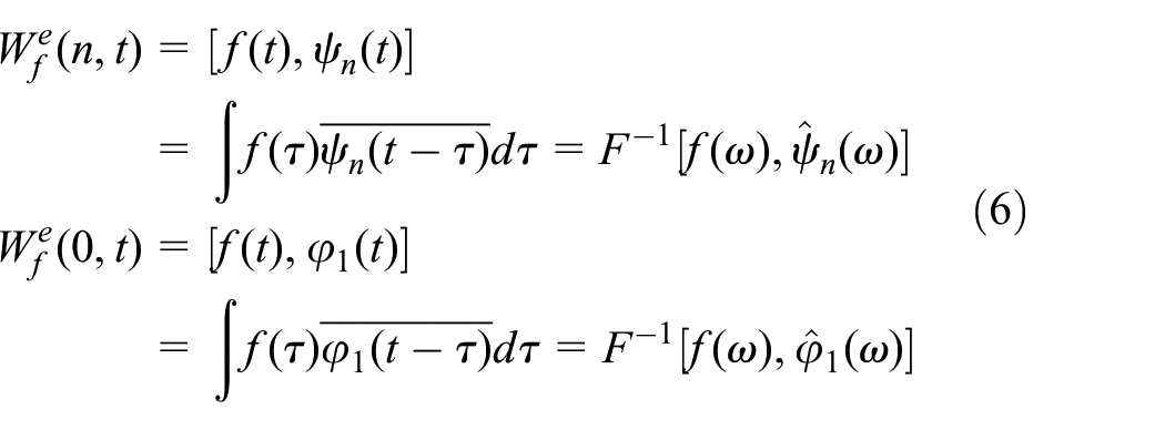
Data-driven RUL prediction can automatically infer causal relationships hidden in the data and directly extract degenerate features of complex systems. It can better deal with massive monitoring data and provide accurate RUL prediction results. 4 In some existing studies, the relevant degradation features are mainly extracted from the time-frequency domain. Wavelet packet decomposition (WPD), 5 empirical mode decomposition (EMD), 6 and Hilbert-Huang transform (HHT) 7 are used to capture the degradation trend of bearings by constructing a health index (HI).
However, a large number of degenerate features not only require expert experience, but also easily lead to feature redundancy. Neural networks can capture small changes in the bearing degradation process and are used by many scholars. Refs,8–10 based on convolutional neural network (CNN) to extract the degradation features of mechanical equipment for RUL prediction. Yoo and Baek 11 build HI based on continuous wavelet transform (CWT) to synthesize time-frequency image features, and CNN is used to build a model. Recurrent neural networks (RNN) 12 and its variants long short-term memory networks (LSTM)13,14 are also used for RUL prediction.
With the development of deep learning, more related algorithms are applied to estimate RUL. The use of deep networks improves the predictive performance of HI. Existing studies have shown that deep learning combined with different neural networks can achieve good results in RUL prediction. However, there is still room for improvement in bearing life prediction methods based on deep networks. Moreover, most of the existing researches directly process the original vibration signal and construct the HI through the original signal (or original Fourier spectrum, edge spectrum, etc.). In practical engineering applications, due to environmental noise and signal attenuation, the fault signal of rolling bearing is often very weak compared with the strong background noise. Especially in the early stage of bearing operation, the fault signal is often annihilated by the background noise. 15 Therefore, if the weak fault features of the bearing are extracted from the raw vibration signal, the prediction accuracy of RUL can be further improved, and the adaptability of the algorithm under different working conditions can also be improved. 10
Aiming at the above problems, a new bearing RUL prediction method based on improved empirical wavelet transform (IEWT) weak fault feature extraction is proposed in this paper. Firstly, the collected bearing vibration signal is divided adaptively by EWT. The spectrum is re-divided and combined according to the mutual information (MI) value to reduce the number of frequency bands and overcome the problem of too much spectrum division of EWT. Secondly, minimum entropy deconvolution (MED) is used to reduce the noise of the reconstructed signal. Six features of wavelet packet entropy, root mean square, variance, frequency kurtosis, frequency skewness, and energy are extracted from the denoised empirical mode functions (EMFs) to characterize the bearing degradation. Finally, a 1D-CNN is used to predict the RUL.
The organization and layout of the rest of this paper are as follows: Section 2 introduces the basic structure knowledge of IEWT and CNN; Section 3 explains the construction of the model in this paper and the evaluation indicators used; Section 4 presents the specific experimental process and experiments results; the last section is the conclusion of this paper and a prospect for future work.
Preliminaries
Improved empirical wavelet transform
EWT is an adaptive analysis method based on the wavelet theoretical framework. The method firstly divides the spectrum of the original vibration signal, constructs a set of adaptive wavelet filter bank, and then analyzes the different frequency components to extract the signal with tight support characteristics. After the original signal is processed by EWT, the signal-to-noise ratio can be effectively reduced and the signal quality can be improved.
Firstly, the fast Fourier transform (FFT) is performed on the original vibration signal to obtain the frequency spectrum. The frequency range is defined as

Where,
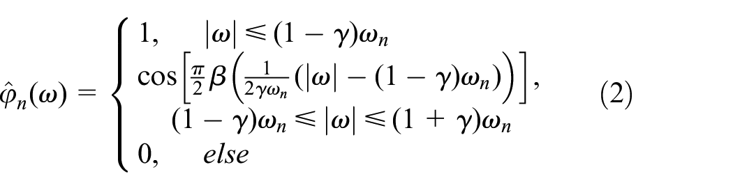

Where,

From the above analysis, it can be seen that the core of EWT is to reasonably divide the Fourier spectrum, that is, to accurately find
Among them:
Based on the above formula, the reconstructed signal of the original vibration signal can be expressed as:

In the above formula: *represents the convolution operation,
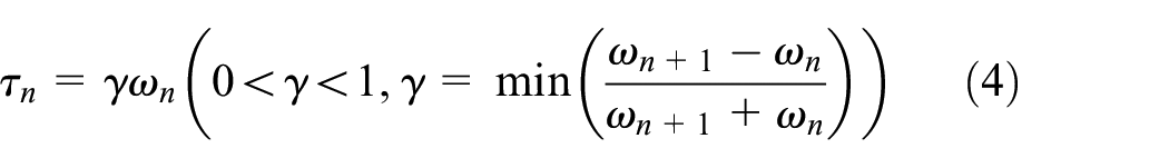
The traditional EWT adopts a scale-space method to adaptively divide the spectrum to obtain the initial demarcation point. However, the number of demarcation points obtained at this time is large, and the frequency bands divided by the spectrum are too many, which brings inconvenience to the subsequent analysis. In this paper, the frequency band is re-partitioned by mutual information value according to the reference. The adjacent frequency bands whose component mutual information value is greater than the average value are merged into the same frequency band, and the adjacent frequency bands whose component mutual information value is smaller than the average value are merged into one frequency band.
Mutual information is used to measure the uncertainty difference between two random variables. It can measure the degree of correlation between two random variables and is more accurate than the correlation coefficient. 16 The mutual information between variable X and variable Y is defined as follows:

Among them:
Figure 1 is the flow chart of IEWT reconstruction signal. The process of IEWT spectrum allocation is as follows:

IEWT reconstruction signal flow chart.
Minimum entropy deconvolution
The vibration signal of rolling bearing is decomposed by IEWT to obtain discrete modal components. In order to extract the more obvious shock signal in the signal, the component with larger kurtosis value is selected to reconstruct the signal. Applying MED to extract shock signals from mixed multi-source interference signals can effectively reduce the impact of acquisition paths on signal attenuation, and further highlight the shock characteristics of vibration signals. It has achieved good analysis results in the extraction of rolling bearing fault features. The specific content of the algorithm can be found in Ref. 16. The bearing vibration signal after denoising by MED can better reflect the degradation state of the rolling bearing in this life cycle, which is conducive to better evaluation of its RUL.
1D-CNN
CNN is a very popular deep learning framework model with powerful feature extraction capabilities and has achieved good applications in image recognition, natural language processing, and other fields. CNN mainly consists of three main parts: convolutional layers, pooling layers, and fully connected layers.
The function of the convolution layer is to perform a convolution operation on the input data and the local area of the convolution kernel, and make the local receptive field traverse the entire input data by sliding the convolution kernel window. The convolution formula is defined as follows:

In the above formula:

Activation function.
The role of the pooling layer is down sampling, which reduces the dimensionality of the feature map while manipulating the most important signals. The max pooling expression is as follows:

Among them:
In the CNN structure, one or more fully connected layers are connected after multiple convolutional layers and pooling layers. Each neuron in the fully connected layer is fully connected with all neurons in the previous layer. Connection layers can integrate local information from convolutional or pooling layers.
Experiment framework
In this section, the details of all the steps of the introduced RUL prediction will be discussed. The specific experimental framework is shown in Figure 3 below.

Experimental framework flow chart.
Firstly, IEWT is used to adaptively divide the bearing vibration signals and the appropriate EMF is selected based on the kurtosis value for signal reconstruction. Secondly, MED is applied to the reconstructed signal to reduce noise. Six characteristic indexes of wavelet packet entropy, root mean square (RMS), variance, frequency kurtosis, frequency skewness, and energy are extracted from the optimal EMF. Finally, the 1D-CNN is introduced to predict the RUL.
In the 1D-CNN structure, the size of the first convolution kernel is 6 * 1 and the stride is 6. Each kernel computes and operates on 6 features simultaneously, and the convolutional layer is followed by a corresponding max-pooling layer to reduce computation. The ReLU function is used as the activation function.
Bearing degradation feature extraction
The degenerate features are extracted from the reconstructed signal, including root mean square (RMS), energy, variance, frequency kurtosis and frequency skewness, and wavelet packet entropy. The extracted feature expressions are shown in Table 1.
Extracted feature index.

Where,
Percentage of remaining life
Set the life label of the

In formula (11),
Evaluation index
In this paper, the following five metrics are used to measure the predictive performance of the proposed predictive model: mean absolute error (MAE), root mean squared error (RMSE), correlation index (


In formulas above,
Experiment verification
Dataset description
In order to verify the effectiveness and superiority of this method in dealing with the rolling bearing RUL prediction problem, two experimental datasets are used to verify the experiments.
FEMTO-ST dataset (IEEE PHM 2012)
The experiments collected different working conditions on the PRONOSTIA 18 platform as shown in Figure 4. The horizontal vibration signal frequency is 25.6 kHz and is recorded every 0.1 s. The sampling interval is 10 s. The specific sampling description is shown in Figure 5 and Table 2.

PRONOSTIA experimental platform.

Sensor data collection process.
Test bed condition information.

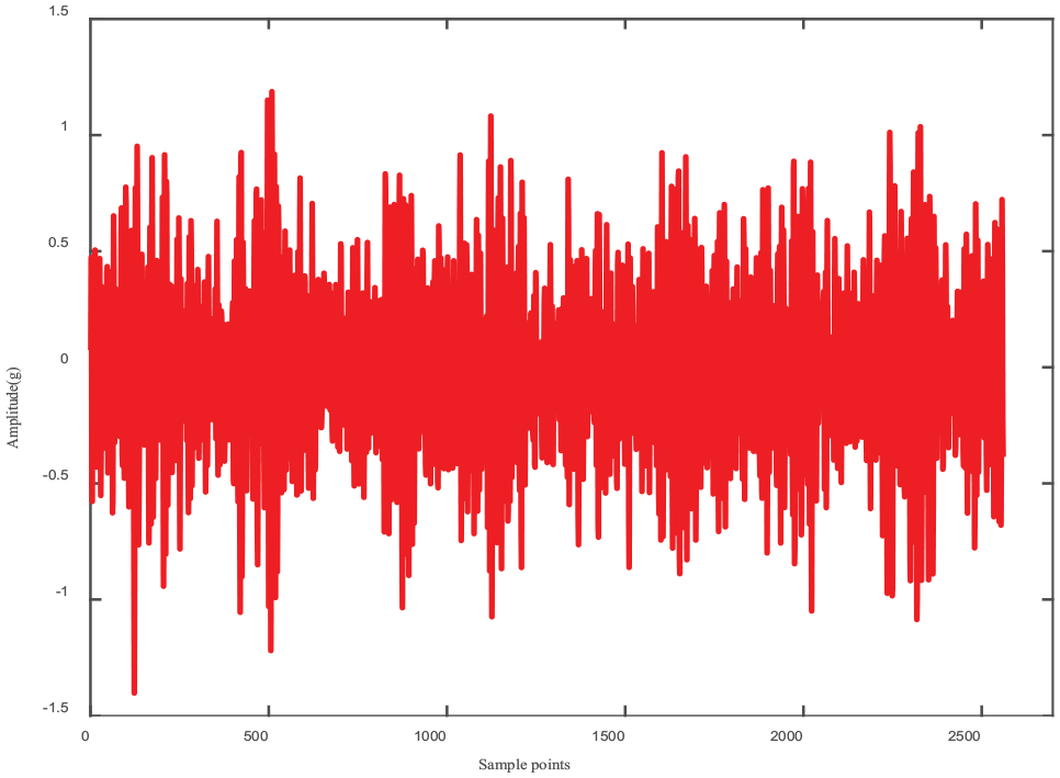
The original vibration signal of the bearing 1_1 during its entire service life is shown in the Figure 6. The horizontal and vertical coordinates represent time and vibration amplitude. As time goes by, the amplitude of the bearing vibration signal gradually increases, indicating that the signal has a rich diagnosis useful information.

Raw vibration signal of PHM Bearing 1_1.
XJTU-SY Dataset
The XJTU-SY dataset 19 contains the full life cycle vibration signals of 15 rolling bearings under 3 working conditions. The experimental platform is shown in Figure 7. The sensor sampling frequency is 25.6 kHz, and the sampling interval is 1 min. Each sampling time is 1.28 s, and each sampling point is 32,768. Table 3 gives a detailed description of the dataset. Figures 8 and 9 are diagram of the sampling process and original vibration signal, respectively.

XJTU-SY dataset experimental platform.
Condition information.


Sensor data collection process.

Raw vibration signal of XJTU-SY Bearing 1_1.
Experiment procedure
Take the PHM bearing 2_7 dataset as an example to illustrate the effect of IEWT. Figure 10 shows the initial 16 frequency bands obtained according to the scale-space method. Based on the initial demarcation point, the frequency bands are re-divided according to mutual information, as shown in Figure 11 below.

Initial frequency band.
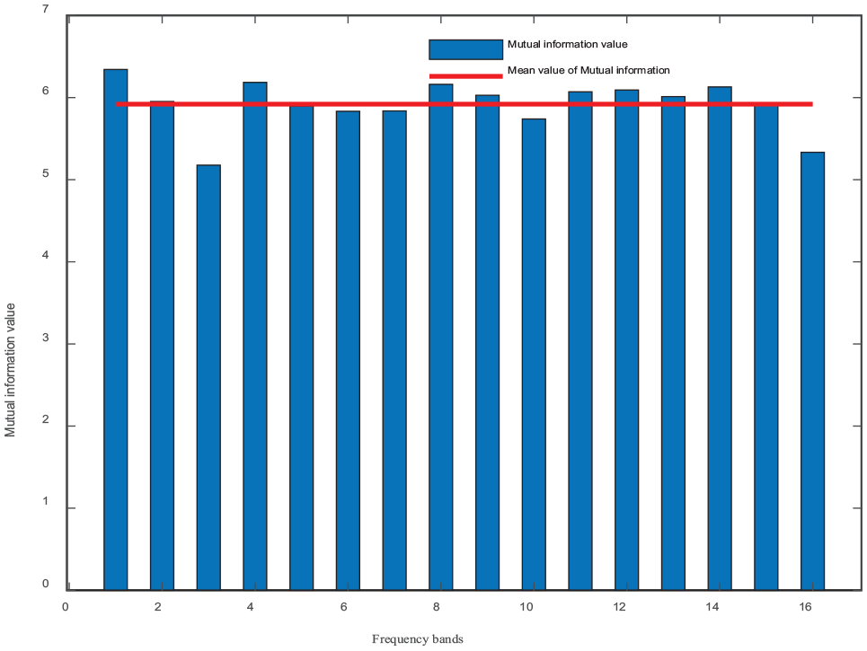
Mutual information value of each frequency band.
The spectrum is re-divided according to the component mutual information in the above Figure 12, and the adjacent frequency bands whose mutual information value is greater or less than the average value are combined to obtain the re-divided spectrum from left to right. The number of bands has been reduced from 16 to 6. Figure 13 is a time domain plot of the repartitioned components.

Re-divided frequency band.

Time series plot of the new component.
Figures 14 and 15 are the original bearing vibration signal and the reconstructed signal after IEWT processing. Figures 16 and 17 are the Fourier spectrum of original vibration signal and reconstructed signal. After filtering out the optimal component of IEWT, the interference of noise and other interference is suppressed. The extracted component signals preserve the main fault information of the bearing. Therefore, the constructed factor can more effectively reflect the bearing failure characteristics and thus better predict the remaining life of the bearing. The corresponding six feature indicators are calculated for each collected data, and the percentage of remaining lifespan is used as a tracking indicator for 1D-CNN training.

Original vibration signal.
Reconstructed signal.

Fourier spectrum of original vibration signal.

Fourier spectrum of reconstructed signal.
A 1D-CNN model is constructed to estimate the RUL as shown in Figure 18. The hidden hyperparameters of CNN are robust. The CNN structure used in this article has seven layers, including three convolutional layers, two maximum pooling layers, and two fully connected layers. The experiment was performed using Windows 10 (Microsoft, USA) system, the central processing unit (Central Processing Unit, CPU) used a 1.80 GHz i5 processor, the memory was 8GB, and the experiment software used MATLAB 2019a (MathWorks, USA) version.

The typical 1D-CNN architecture.
Experiment results
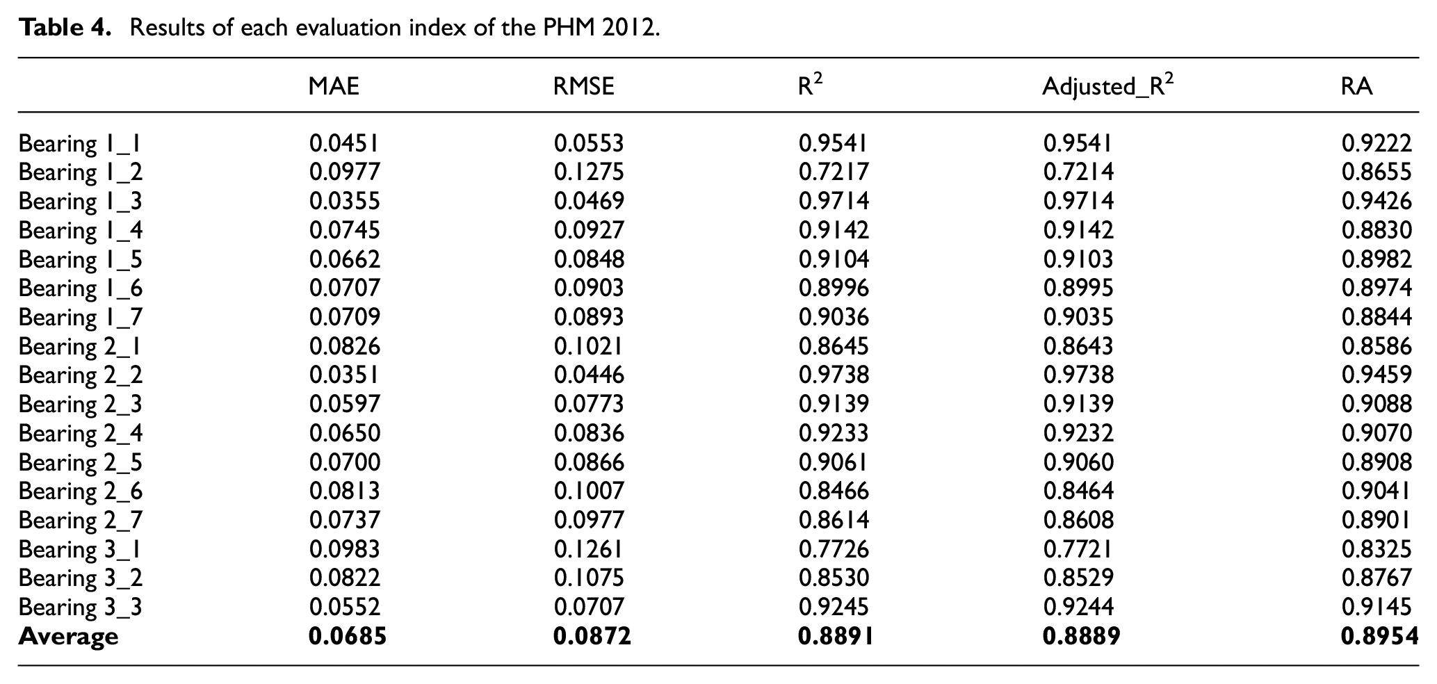
Each time the data passed into the 1D-CNN structure is normalized 6-dimensional feature data. During the training of the 1D-CNN, the optimizer uses the “adam” optimizer, which runs for 200 iterations. Through the leave-one-out method test, the results of the five evaluation indicators of each bearing are as follows Tables 4 and 5.
Results of each evaluation index of the PHM 2012.
Results of each evaluation index of the XJTU-SY.

For the PHM 2012 dataset, it can be seen that the prediction effect under the three working conditions is still relatively consistent, and the trend of the remaining life of the bearing can be better predicted. The load of the first working condition is 4 kN, which is relatively low in the comparative experimental load, so the bearing running time is relatively long. The collected training data is longer, so the training model is more effective. In the same experiment, the third condition had the largest load. The corresponding bearing has a shorter operating time and less data is collected. The samples trained by the 1D-CNN model are greatly reduced, and the error of the corresponding model is relatively large, but it is still within an acceptable range.
For the XJTU-SY dataset, the radial load of working condition 1 is 12 kN, which is the largest in the same experiment and the corresponding speed is the lowest. The radial load of working condition 3 is 10 kN, the maximum speed is 2400 r/min, and the collected data is also the most. Figures 19 and 20 are renderings of rolling bearing RUL predictions under different operating conditions in the two datasets.

PHM 2012 dataset predicted result. (a) PHM bearing 1_1 predicted result, (b) PHM bearing 2_2 predicted result, (c) PHM bearing 3_1 predicted result, (d) PHM bearing 3_3 predicted result.

XJTU-SY dataset predicted result. (a) XJTU-SY bearing 2_1 predicted result, (b) XJTU-SY bearing 2_3 predicted result, (c) XJTU-SY bearing 3_3 predicted result, (d) XJTU-SY bearing 3_5 predicted result.
As a comparative experiment, EMD, stationary wavelet transform (SWT), and variational mode decomposition (VMD) are selected to compare with IEWT. And in order to show the robustness of 1D-CNN, LSTM is selected for comparative experiments. In the experiments, the number of EMD layers is adaptive. The number of SWT layers is 3, and the wavelet basis is “morlet.” The number of VMD layers is 5. The number of nerve cells in each hidden layer of LSTM is 150, and the number of hidden layers is 5.
In the selected PHM dataset, the corresponding average value of the evaluation index calculated for each bearing is calculated, and the results are shown in the Table 6. The MAE for IEWT-CNN, EMD-CNN, SWT-CNN, VMD-CNN, and IEWT-LSTM are 0.0685, 0.0814, 0.1196, 0.0719 and 0.0726, respectively. Comparing the other four methods, the MAE proposed in this paper decreased by 15.85%, 42.73%, 4.73%, and 5.64%, respectively.
Evaluation index comparison for PHM 2012 dataset.

In the selected XJTU-SY dataset, the evaluation index of each bearing and the corresponding mean value are calculated. The results are shown in the Table 7. The MAE of the method proposed in this paper is 0.0451 and the RMSE is 0.0523. Among them, MAE, RMSE, and MAPE are all smaller than the prediction results obtained by EMD-CNN, SWT-CNN, VMD-CNN and IEWT-LSTM. Moreover, R2, adjusted_R2, and RA are all higher than the prediction accuracy of the above four models, indicating that the model proposed in this paper is superior to the above four models. Compared with several other methods, the complexity of the model is also relatively low, and the running time is relatively fast.
Evaluation index comparison for XJTU-SY dataset.

Conclusion
In this paper, A new method for rolling bearing RUL prediction based on IEWT weak fault feature extraction and 1D-CNN is proposed to overcome the interference of noise and other disturbance signals. Firstly, the bearing vibration signal is adaptively divided by EWT, and the frequency bands are re-divided according to the mutual information value to reduce the number of frequency bands. Secondly, some appropriate components are selected according to the kurtosis index, and deconvolution with minimum entropy is used to reduce the noise of the reconstructed signal. Six feature metrics are extracted from the denoised EMF. Based on the constructed feature metrics, a 1D-CNN is applied to predict the RUL of rolling bearings. Finally, based on the validation on two public rolling bearing datasets, the proposed bearing RUL prediction method has higher prediction performance.
In the future, this method will be applied to more industrial scenarios, including gearboxes and aero-engines, etc. In addition, some other methods of adaptively extracting features to construct HI should be applicable. Other potential degradation metrics will try to combine with the CNN model for higher health prediction accuracy. Future work also includes applying the proposed framework to a wider range of case studies on experimental data in other applications, as well as investigating other potential degenerate labels to achieve higher RUL estimation accuracy.
Footnotes
Handling Editor: Chenhui Liang
Declaration of conflicting interests
The author(s) declared no potential conflicts of interest with respect to the research, authorship, and/or publication of this article.
Funding
The author(s) disclosed receipt of the following financial support for the research, authorship, and/or publication of this article: This work was supported in part by the National Natural Science Foundation of China under Grant 61671338 and Grant 51877161 and Open fund of Hubei Key Laboratory of Metallurgical Industry Process System Science (No. Y202007).