
Abstract
Despite the rapid development in very recent years of Artificial Intelligence models to predict poverty risk, this problem still remains an unsolved open challenge, especially from a multidimensional perspective. One of the main challenges is related to the scarcity of labelled and high-quality data for training models coupled with the lack of a general reference model to build good predictors. This results in the proposal of a variety of approaches tailored to specific contexts. This paper presents our proposal to address multidimensional poverty prediction, starting from an unlabelled dataset. We focus on the case of a fragile population, the older adults; our approach is highly flexible and can be easily adapted to various scenarios. Firstly, starting from expert knowledge, we apply a stochastic method for estimating the probability of an individual being poor, and we use this probability to identify three levels of risk. Then, we train an XGBoost classification model and exploit its tree structure to define a ranking of feature relevance. This information is used to create a new set of aggregated features representative of different poverty dimensions. An explainable novel Naive Bayes model is then trained for predicting individuals’ deprivation level in our particular domain. The capacity to identify which variables are predominantly associated with poverty among older adults offers valuable insights for policymakers and decision-makers to address poverty effectively.
Introduction
Poverty, as highlighted by the Organization for Economic Cooperation and Development (OECD), is undeniably one of the most significant social problems of our global community. It is crucial to recognise that poverty impacts not only developing countries but also vulnerable groups within all societies. The Council of Europe 2 reveals the profound correlation between poverty and human rights, emphasising that extreme wealth imbalance results in extreme inequality in the realisation of fundamental human rights. Therefore, addressing poverty is tied to mitigating this inequality, and being able to predict it becomes a crucial first step in defeating it. The application of AI to the problem of poverty prediction represents a recent development, with significant early work published in 2016 [26], and a rapid increase in interest in 2021 [44]. The increasing use of AI in addressing poverty, and more broadly, in achieving the Sustainable Development Goals, particularly over the past two years, is closely related to the cumulative impacts of the COVID-19 pandemic, the Russia-Ukraine conflict, and climate change [9, 40]. At first, poverty and its corresponding indicators were considered solely in relation to monetary aspects, mainly measuring income-related indicators [7, 21]. However, recent developments recognise that poverty is the product of a multifaceted interaction of various aspects, requiring the definition of multidimensional indicators [42, 43]. The concept of multidimensional poverty includes several definitions and measurement methodologies, reflecting different approaches to data collection and analysis. Moreover, addressing the needs of vulnerable populations requires the identification of suitable measures capable of capturing their peculiarities.
The research presented in this paper is related to the
In this paper, we present our classification approach aimed at identifying three levels of poverty risk, considering the following key issues: Pre-process the collected data to ensure data quality and remove noise from the features used to feed ML algorithms; Apply a procedure to automatically assign labels to the collected data, starting from preliminary information acquired from domain experts and taking into account the multifaceted aspects of poverty; Identify which are the features that are mostly relevant to predict poverty risk; Apply different supervised Machine Learning models on a set of aggregated features selected from the relevant ones; Identify the variables that are mainly responsible for predicting poverty in the elderly population, thereby directing the efforts of policymakers and municipalities to prevent and effectively address it.
The paper is organised as follows. A preliminary analysis of the state of the art is reported in Section 2, considering the role of AI in predicting multidimensional poverty. Subsection 3.1 presents the
State of the art
Despite poverty being a well-recognised issue, the use of AI models for predicting poverty remains relatively recent, with notable developments observed since 2016 [11, 26], and experiencing a considerable acceleration starting from 2021. Literature reviews or surveys systematically evaluating the contribution of AI within this field are scarce [25, 44]. Particularly, the contribution of AI models has become increasingly significant in recent years, in conjunction with a shift in perspective on poverty, which has progressively been acknowledged as a multidimensional issue intricately tied to various facets and unique characteristics of the targeted population, including factors such as age and geographic location. Multidimensional measures of deprivation include diverse indicators fitting into a synthetic scale [12, 14], which is deemed to reflect basic living standards and the inability to meet the minimum acceptable way of life in one?s own society. Several methodologies for assessing poverty from a multidimensional perspective exist, including those aiming to aggregate data from different sources, and statistical approaches, i.e., principal component analysis, or cluster analysis [4], which are considered appropriate when they effectively capture the joint distribution of deprivations, identify those experiencing poverty, and yield a single cardinal figure for evaluating poverty levels.
One major challenge in predicting poverty using AI lies in the scarcity of high-quality labelled data. Various proxies, such as the Proxy Means Test (PMT) labels, can be considered as ground truth for ML training. However, these proxies are not easily verifiable [33]. Traditionally, datasets for poverty prediction are related to demographic and livelihood indicators [1], household surveys [5, 39], or remote sensing data, such as satellite images or geospatial data [23, 28], but to the best of our knowledge, no dataset at a subject-based level has been shared with the research community. Among different ML techniques for poverty classification, decision tree [39, 47], random forest [13, 33], and ensemble approaches [1, 48] are the most used.
The pioneering work by Jean et al. [26] proposed to analyse high-resolution satellite images to predict poverty considering a Convolutional Neural Network (CNN) model pre-trained on ImageNet, and the more recent work of Wijaya et al. [46] applied a deep neural network to estimate city-level poverty starting from e-commerce data, considered as indicators of consumption and purchasing power. Despite these advancements, deep learning models have not been widely adopted, instead, traditional machine learning approaches based on hand-crafted features and explainable AI models [49] are preferred. These approaches excel in identifying specific characteristics associated with poverty, which is essential for developing targeted poverty prevention strategies. In line with this, AI models have been applied for feature selection [41] and feature ranking [6] to create models that rely only on the most important variables [39].
Materials and methods
The AMPEL Dataset
A questionnaire designed by domain experts was administered to senior adults by trained interviewers, to gather data on various aspects of their living conditions. We have considered several measures and multidimensional poverty indexes as well as standardised questionnaires. Finally, we decided to follow the social inclusion approach introduced in [42]. An individual can be poor, that is, socially excluded, despite having adequate income [35], when they do not participate in key activities of the society in which they live. In fact, the concept of exclusion refers to the systematic exclusion of individuals, families, and groups from economic, political, and social activities that are fundamental to the quality of life [22, 28]. Based on these theoretical justifications, therefore, it was decided to prepare a questionnaire aimed at measuring the many factors that contribute to the material and social deprivation of older people, namely: socioeconomic conditions (economic stress, material deprivation, housing conditions); difficulty in accessing health care and services; health (general health conditions, physical and sensory limitations, chronic diseases and conditions, risk factors, psychological well-being) [36]; daily life (social support, generalised trust, safety, social relationships, participation in social activities); and subjective well-being.
The resulting questionnaire thus covered topics such as monetary aspects, environment, social networks, and quality of life, with a total of 125 variables (features) for each individual. The questionnaires were administered to 496 people, (336 females) with an average age of 76.4 (standard deviation = 8.9). The questionnaire in the original Italian version, together with its English translation are available to the research community 4 . Both the questionnaire and the protocol chosen to administer it have been reviewed and approved by the Research Ethics Committee at The University of Milano-Bicocca, Italy.
The geographical distribution of the elderly subjects considered in our study is illustrated in both Table 1 and Fig. 1.
Target municipalities for the AMPEL dataset
Target municipalities for the
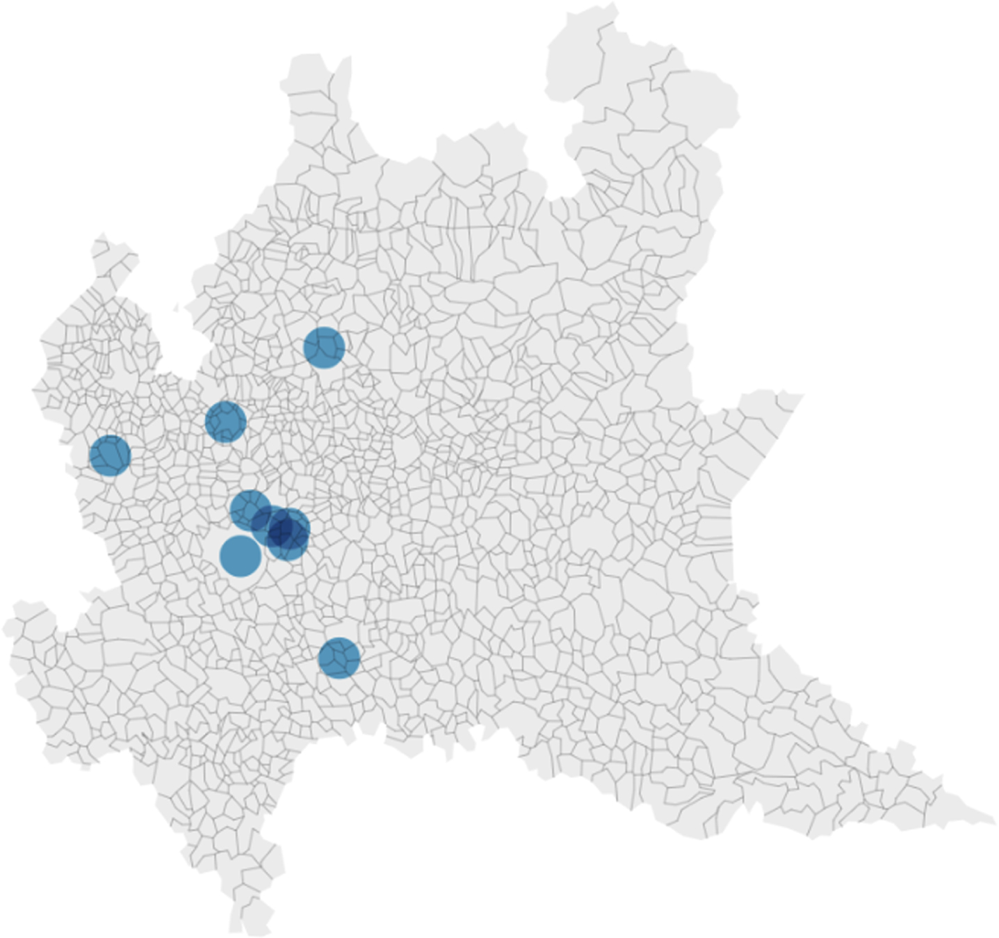
Map of the considered municipalities in Lombardy - Italy.
The collected variable type can be i) Categorical variables, which assume a fixed set of values and include binary variables (e.g., private health insurance coverage: yes or no), or ii) Numerical variables, which can be either discrete (e.g., the number of individuals that live in a house) or continuous (e.g., the height and weight of a person). It should be noted that in the collected dataset, the numerical features are considerably less than the categorical ones, a topic that will be addressed in Section 3.3.
The collected variables captured by the questionnaire can be grouped in 5 different categories as suggested in [42]:
The prediction of multidimensional poverty using innovative AI based solutions requires addressing methodological challenges to face the complexity of the task, especially in cases in which the dataset comprises a limited sample size (496 individuals) and includes missing values due to participant information gaps. In this Section, a methodology is presented to address these critical data issues and the lack of labelling. This approach is illustrated through a pipeline of four distinct phases, as in Fig. 2: The proposed framework.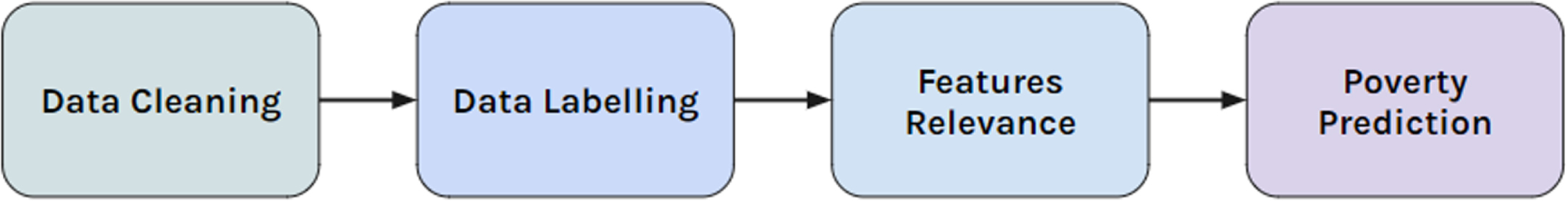
This dataset requires essential preliminary data pre-processing steps to clean and normalise the data entries. Firstly, generalities and irrelevant features, such as those with an excessive number of missing or noisy values, are removed. When possible, missing values are filled with relevant ones. For instance, if an individual lacks a specific condition and does not answer the relevant question in the form, all such entries are thus filled with a categorical value representing the absence of that specificcondition.
The dataset comprises data collected from a survey, including features that are answers to open-ended questions, presenting considerable name heterogeneity, with answers that are semantically equivalent but syntactically different. To mitigate this effect, whenever feasible, semantically similar values are mapped to a common one.
Related and dependent features represent another significant issue in this dataset. To reduce redundancy, the dataset is simplified by grouping redundant features into a single meaningful one.
The majority of the features in our dataset are categorical, and only a few are numerical, such as age or number of cigarettes smoked weekly.
Considering the small number of observations in this dataset, namely 496, the numerical features are simplified, reducing their information by binarising their values. For example, instead of representing the number of people living with an individual, a possibly challenging numerical value to handle in a categorical dataset, this information is transformed into whether this individual lives alone. This type of feature engineering is applied with the same logic over all the numerical features remaining in the dataset, thus transforming it into an entirely categorical dataset. The steps illustrated above are repeated on the whole dataset and allow reducing the number of features from 125 to 103. From a computational perspective, this feature reduction may not be significant, but it could help to eliminate some noise, enhancing the quality of the classification results and providing better explainability.
Data labelling
Due to the absence of a standard definition and a specific indicator of multidimensional poverty, the challenge lies in determining the poverty risk level of each individual in the dataset to build a ground truth on which Machine Learning prediction models can be trained.
This issue has been solved by applying the framework described in a previous study [20] and originally proposed by Liberati et al. [30]. This approach assesses the likelihood of poverty for each individual by considering a weighted sum of the deprivation indices associated with each feature (established through a cut-off value). Instead of defining a fixed importance weight vector, this technique builds an embedded representation at the individual level, obtained by randomly sampling the weight distribution and evaluating an aggregated index. This procedure is crucial for classifying individuals within the dataset into three poverty levels: high (represented with red colour), medium (yellow colour), or low (green colour) depending on the resulting index distribution. As mentioned above, the implementation follows the methodology reported in [20], with adjustments made to the initial deprivation cut-offs to align with the characteristics of the new dataset. All the details of the implementation of this labelling method are reported in [20], but to understand how the vector space has been built, all the steps have been summarised below (and illustrated in Fig. 3): Data labelling: the first matrix represents for each row a subject, for each column a feature. The second matrix is the Deprivation Matrix, obtained by applying the cut-offs defined by the domain expert. This matrix is multiplied with a matrix of weights to obtain the Deprivation Score Matrix. Our procedure extracts 10000 different weight vectors from a uniform distribution. In the example reported in figure, m = 4. The last matrix is the Poverty Indicator Matrix, which reports the poverty rank, of each individual within the considered population.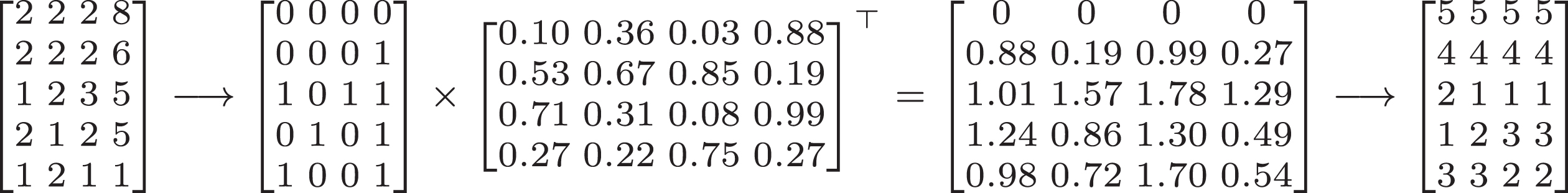
Using their ranking distribution, reported in the Poverty Indicator Matrix, individuals can be classified into three levels of poverty, high (visually coded with red colour), medium (visually coded with yellow colour) or low (visually coded with green colour).
To qualitatively analyse the results of this labelling procedure, we show, in Fig. 4, the distribution of individuals belonging to different classes, for increasing sample size m. Here the 2D spatial representation of the embedding vectors using TSNE [45] (T-distributed Stochastic Neighbor Embedding) is visualised. TSNE is a dimensionality reduction technique, commonly used in ML and data analysis for visualising high-dimensional data in a lower-dimensional space. In particular, we report how vectors representing individuals of different classes are distributed in the embedding representation space considering m equal to 5, 10, 50, 100, 1000 and 10000 respectively. We note that by increasing m, the three groups of individuals tend to cluster and become visually distinguishable in the representation space.
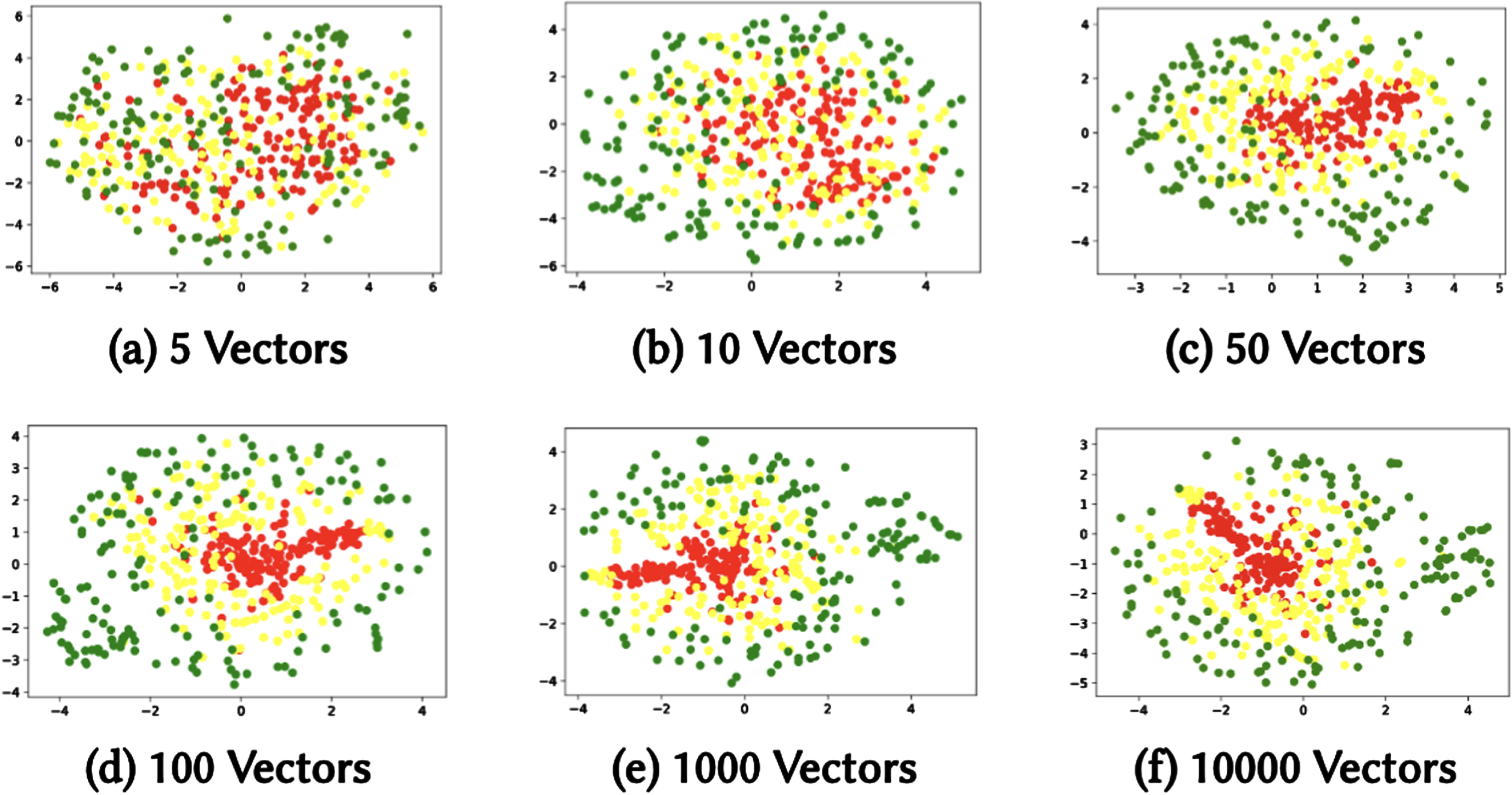
TSNE representation of vector spaces by varying the number of weight vectors.
This behaviour better explains the advantages of employing a set of randomised vectors:
Using a sample size m adequately high allows the model to reach stable results in terms of label assignment to individuals, as shown in Table 2.
Groups size depending on number of weight vectors
One of the relevant aspects of this project is to understand the contribution of features belonging to different domain dimensions, to an individual’s poverty. To address this issue, we analysed the feature correlation through Cramer’s V [18], a measure of association between two nominal variables based on Pearson’s χ2 test. We observed that the only significant correlations are observed among features related to health status (HS). Therefore, to obtain an estimation of the feature relevance, we trained a machine learning model on the labelled dataset. In particular, the Information Gain value of each feature in the tree-based model XGBoost [15] was investigated.
Once fitted to the data, an XGBoost model can return the importance of each feature based on its contribution in predicting the right label. This importance can be defined following various metrics; in this case, particular interest lies in the gain score of each feature, defined as the average gain across all splits the feature is used in. The gain of a specific feature represents its relative contribution to the classification of each tree in the model; it quantifies the amount of information gained about the target class after adding the relative split in the model.
The information gain of a tree-based model is a powerful metric, but it can be biased, especially in case where the dataset has a large number of features (103 after the pre-processing step) and a low number of observations (496). In such circumstances, the model is at high risk of overfitting, as verified by our experiment 5 .
To address this issue, a 5-fold cross-validation process is adopted. The dataset is initially divided into two subsets: 80% is used for training, while the remaining 20% is retained for testing. In the training subset of the dataset, a 5-fold cross-validation of the XGBoost model is carried on, and all of the 5 models fitted in the process are saved, along with their gain scores. To avoid overfitting, these scores are then averaged across the 5 models. Having computed these scores, it is now possible to rank eachfeature.
In Fig. 5 the variables in the top-10 positions are reported, considering the poverty dimension to which they were assigned by the domain expert (see Section 3.1). In Table 3 a detailed description of each of them is provided, sorted by their averaged gain scores across the cross-validated XGBoost models. The associated questions are reported in the last column. The complete list of the survey questions is made available for the research community in Italian (original version) and in English through the AMPEL Dashboard presented in Section 5.
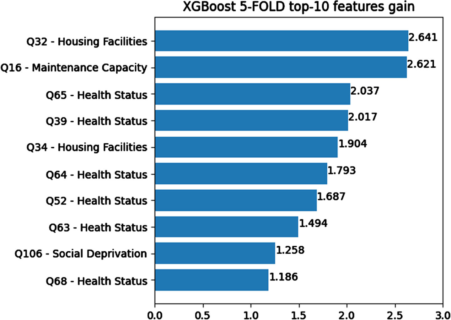
Top 10 features by their gain scores obtained as the average of the scores across the 5 cross-validated models.
Questions corresponding to the first top-10 features
From the analysis of Fig. 5 and Table 3, it emerges that 7 out of 10 among the top-10 features are assigned to the Health Status dimension. This finding is not surprising, as poverty is associated with health-related outcomes, including physical and mental disorders [24]. The presence of multiple conditions, i.e., the comorbidity and multimorbidity status, negatively impacts wealth as people age: the presence of comorbidities was associated with 20–22% wealth loss over three-years [27] and such a negative effect extends from individuals to their networks [32]. Additionally, prevalent mental health conditions, such as depression, act as a booster for multimorbidity and total healthcare expenditure among older adults [17]. Moreover, a clear bi-directional relationship exists between adverse economic situations, health status and disability [8, 19].
The second most relevant variable is related to an overall evaluation of the quality of life, which is consistent with studies that highlight the strong relation between poverty, life satisfaction and happiness [2].
To give more insight, we also computed the relevance of each poverty dimension by averaging the gains of their features. Results, reported in Fig. 6, show a relatively balanced distribution. Despite the abundance of features related to the Health Status in the top-10 rank, depicted in Fig. 5, this dimension is not dominant among the five considered, and the most prominent one is the Housing Facilities.
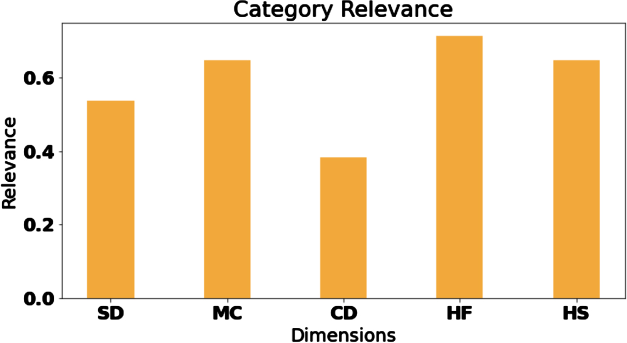
Category Relevance computed using the gain scores obtained from XGBoost. The score has been normalised by the size of each dimension MC = Maintenance Capacity (10), CD = Consumption Deprivation (12), HS = Health Status (41), HF = Housing Facilities (11), and CD = Social and Context Deprivation (12).
Computing the relevance of both single features and poverty dimensions is of paramount importance, as it offers to municipal policymakers valuable insights, guiding them to identify appropriate interventions to effectively address and prevent poverty. In addition, this analysis enables to focus on a subset of questions that should be prioritised when administering a new questionnaire to a different sample of individuals.
Three distinct classification models are examined in this study: XGBoost [16], Categorical Naive Bayes [37] and a novel hybrid approach that combines XGBoost feature gain scores with a Naive Bayes classifier, taking into account the five poverty dimensions defined in Section 3.1.
Through the following analysis, the same 80% portion of the dataset previously used for feature relevance is employed to train the presented models, while the remaining 20% is retained for the testing. Thus, all the models are trained on identical data and assessed on the same test set.
In this Section, the proposed models are evaluated considering three different metrics: accuracy, recall and F1-score.
The XGBoost classification model
Building upon our previous work [20], we seek to leverage the insight gained into the impact of each feature. We first examine XGBoost model in its categorical classification setting. This model provides the baseline for subsequent predictive models, and it is chosen because of several factors: it offers substantial interpretability by visualising the aforementioned feature importance, and both training and inference on the model are remarkably fast. With these considerations in mind, our XGBoost model achieves 79% of overall accuracy across the test set as reported in Table 4.
Performance of the XGBoost classifier
Performance of the XGBoost classifier
To gain more explainablity, we also considered a Naive Bayes Classifier. Naive Bayes models assume conditional independence between the various features of the dataset. Such an assumption is reasonable given that the questions asked to the individuals cover different subjects, albeit sometimes related to the same topic. Once again, the model is trained on the entire training set, achieving slightly better results than the XGBoost model with a global accuracy of 84% as shown in Table 5.
Performance of the Categorical Naive Bayesian classifier
Performance of the Categorical Naive Bayesian classifier
Increasing the number of features tends to add more information to the model. Ideally, this can lead to better discrimination between classes. However, this also has its downsides: as the number of features grows, so does the risk of overfitting the train data: the model might learn unrelated noise while losing the ability to generalise on the test set later.
Naive Bayes classifiers are known for their simplicity and effectiveness in many classification tasks [37]. However, they tend to be less informative as the number of features increases. To create a model as explainable as possible, it can be interesting to study how the model’s performance changes while increasing the number of features it is trained with.
In Fig. 7, we present the performance evaluation of the model employing a 5-fold strategy, showcasing the model performance as we increment the number of features. Note that features have been selected following the order of the average gain score computed on the 5 cross-validated XGBoost models as discussed in Section 3.5.
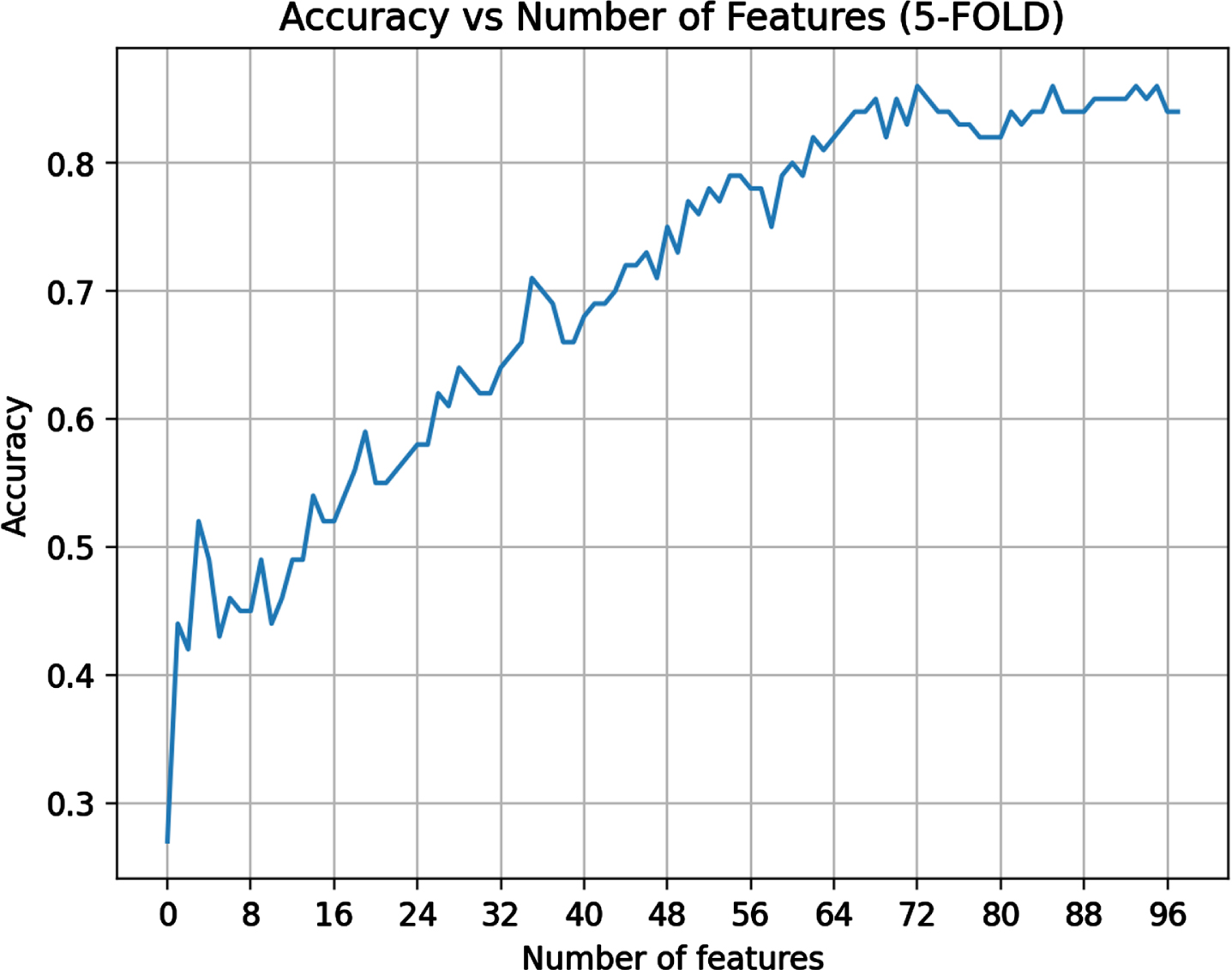
Accuracy of the Categorical Naive Bayes classifier concerning the number of features selected from a list, ordered for the gain scores obtained applying the XGBoost model.
The accuracy trend appears irregular, varying the number of features considered, probably due to the small number of observations in the dataset. However, it is still possible to appreciate the incremental tendency that stabilises around the upper 60 ones.
The purpose of this model’s introduction is to provide a predictive model that is as understandable as possible and that can function in a multidimensional environment using a reduced number of features. These dimensions correspond to the five groups defined in Section 3.1: Social Deprivation, Maintenance Capacity, Consumption Deprivation, Housing Facilities and Health Status.
For each dimension, a new feature is computed by linearly combining the XGBoost information gain of each feature with its relative cut-off defined by the domain expert. To improve the generalisation power of the model, the gain used for this linear combination is the one averaged from the 5 cross-validated models in Section 3.5.
Starting from the binary deprivation matrix defined in Section 3.4, each row describes the features where an individual is considered deprived. These rows are here referred to as deprivation vectors. Each column represents, for a given feature, the distribution of individuals that exceeds the cut-offs defined by the domain expert.
Let us define a as the vector of the feature information gains, i.e. each a
i
with i ∈ {1, ⋯ n} is the gain score of the i-th feature, and let b be the deprivation vector where each b
j
with j ∈ {1, ⋯ n} represents if and individual is deprived or not for the j-th feature. Then we define the individual deprivation score as:
If we group the elements of the deprivation vector into the five poverty dimensions, the resulting values represent the ’magnitude’ of deprivation experienced by the individual in each of the five dimensions.
At this point, each individual is encoded into 5 values that will now be used to determine their poverty class. To this end, a Naive Bayes classifier is applied, having a parent node for each of the 5 classes of features as shown in Fig. 8.
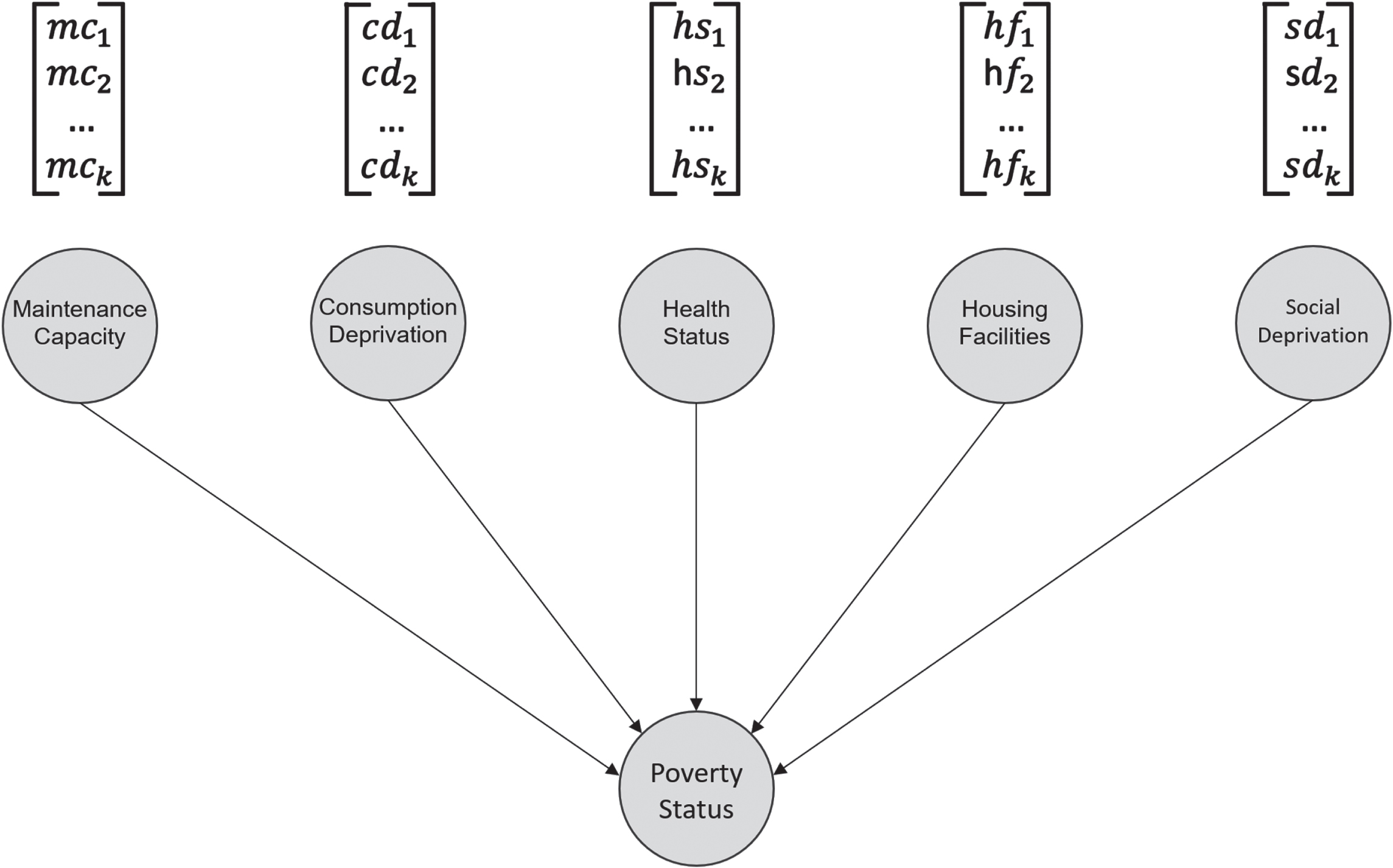
Structure of the Naive Bayes classifier, where each of the 5 parent nodes represents the score in that poverty dimension for each individual.
The classifier built on top of this pipeline shows good performance as reported in Table 6, reaching an overall accuracy of 89% on the test set. It is essential to mention that the test set has never been used in the entire pipeline except for assessing this metric. This result shows how well the model can generalise using the average gain extracted from the cross-validated XGBoost models introduced in Section 3.5.
Performance of the Naive Bayes multidimensional poverty classifier
The project implementation includes multiple independent software modules that cooperate by exchanging data resulting from the analyses described above. Figure 9 shows the different software components implemented and deployed using Docker containers. A brief description of each part is reported below:
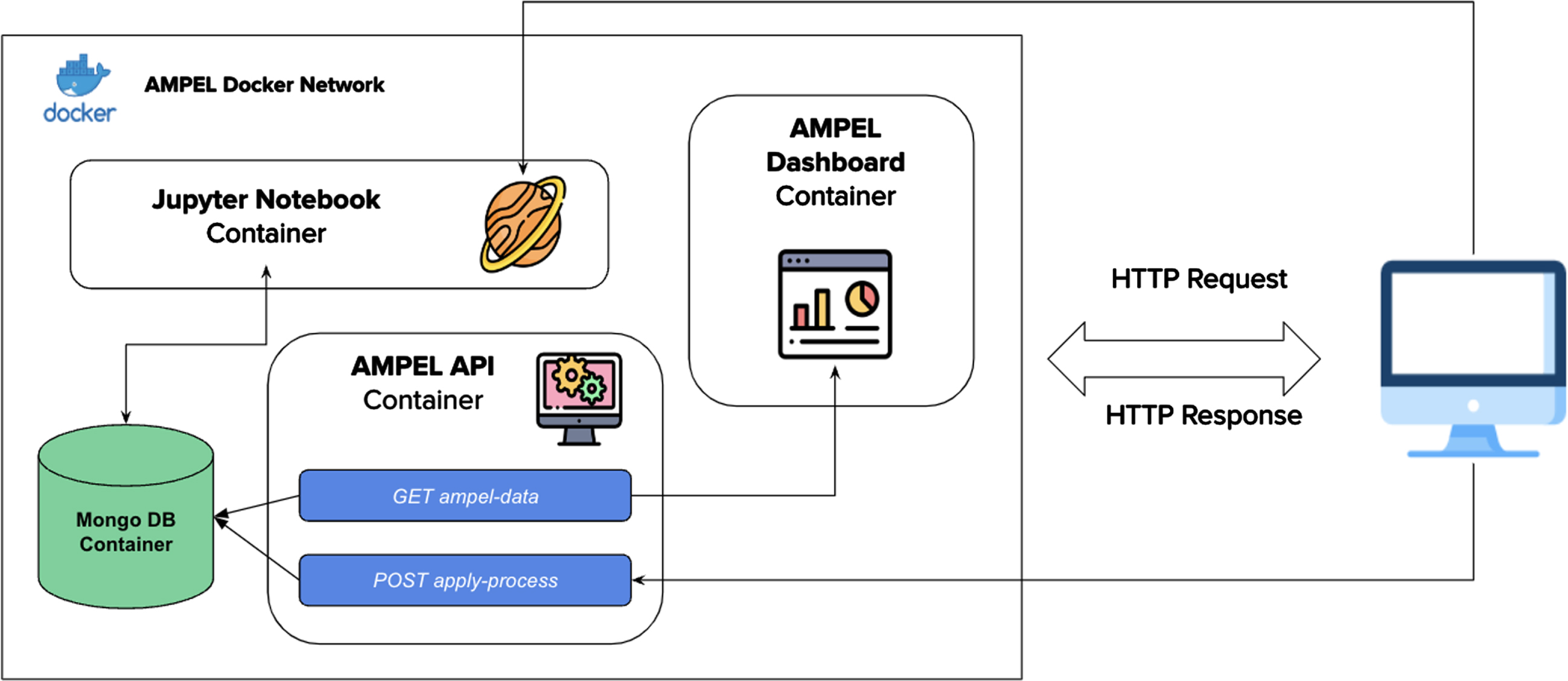
Among the services outlined above, the
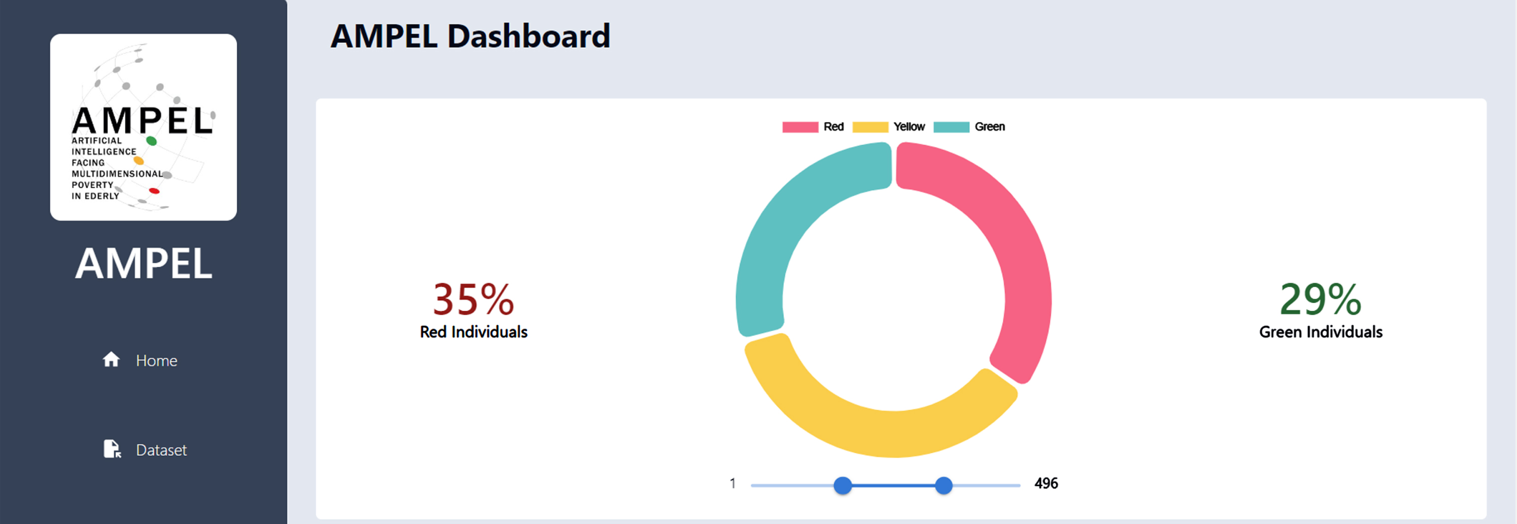
Panel utilised by the domain expert for examining poverty within the population.
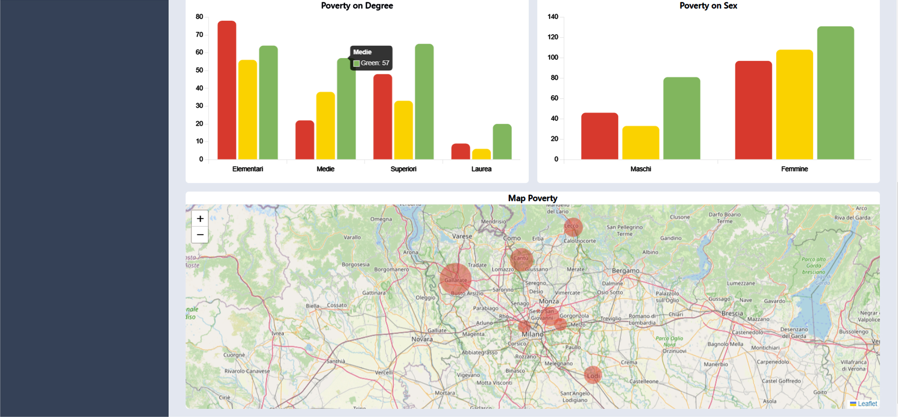
Examples of different data visualisations for data analysis. Top left: distributions of subjects within the three poverty classes, considering different levels of education. Top right: distribution of the subjects within the three poverty classes, considering the gender. Bottom: geographic distribution of the considered subjects.
Among the charts available on the Graph page of the dashboard, the main contributions are:
This work introduces a novel approach to predicting multidimensional poverty using unlabelled data. While encouraging results were achieved, it’s important to acknowledge both the limitations and strengths of this methodology.
Although the dataset is valuable because it focuses on individual subjects rather than demographic or aggregated information such as satellite images or geospatial data, it is important to emphasise the limits of observations.
On the contrary, the data collected refers to subjects distributed within a localised area in Lombardy, Italy. While this may be considered a further limitation, it actually could increase the richness of the information contained in the dataset. It is noteworthy that multidimensional poverty can be described by variables that are strictly related to the peculiarities of the considered population, and a broader sample of subjects may hide some important aspects specific to smaller groups of individuals.
Another notable strength of the proposed approach is its reliance on domain experts’ knowledge, which, while not limiting machine learning in data exploration, reveals new relationships and meaningful indicators in the definition of multidimensional poverty. Specifically, by leveraging the tree structure of XGBoost, it becomes possible to understand which variables are the most relevant for predicting poverty in the target population. Moreover, starting from their relevance, it is feasible to explore high-level poverty dimensions that can better encapsulate the primary aspects involved in poverty creation. In this work, we extracted the feature ranking from cross-validated XGBoost models. However, other approaches like SHAP [31] could be considered and potentially combined together. From preliminary comparisons, our ranking shows partial agreement with the feature rank obtained using SHAP, but more in-depth analysis is needed to better understand thedifferences.
Furthermore, considering each feature separately might not always be practical, for this reason, the Multidimensional Classifier proposed in Section 4.3 enables prediction according to a lower number of poverty dimensions defined by the domain expert. This approach is particularly useful when limited resources for supporting the elderly are available as it facilitates the identification of the main categories for intervention.
The framework here presented is specifically designed to predict various levels of poverty within the elderly population. However, its main advantage resides in its adaptability and potential for generalisation across different contexts. For example, it can be extended to encompass data concerning poverty among various vulnerable populations. In particular, even if different groups of subjects for age or geographic locations are characterised by different features, the same framework can be applied to new data, revealing the relevance of variables directly related to the considered scenario. The framework is not limited to poverty prediction within the elderly population and can be applied in diverse contexts. For instance, it could be employed for the analysis of digital health records to identify different levels of specific pathologies, such as mental decline.
Lastly, a dashboard has been developed as a prominent tool for data visualisation, accessible to the research community along with the collected dataset and codes developed for the analysis.
Conclusion and future work
The proposed AI approaches for predicting multidimensional levels of poverty have demonstrated promising performance. The feature relevance analysis enables the definition of poverty scores based solely on five poverty dimensions, derived from appropriately linearly combined features. This approach allows model training on feature vectors of a reduced dimensionality while retaining valuable information from the original feature set.
However, it is worth acknowledging both the potential biases in the final results introduced by the labelling procedure and the possibility of revising and extending the definition of the five dimensions. To further validate and generalise our proposal, we plan to leverage other labelled datasets available in the literature. This approach will allow us to assess both the labelling procedure and the effectiveness of the proposed Naive Bayes multidimensional classifier.
Conflict of interest
There is nothing to declare.
Footnotes
Acknowledgements
We want to give our thanks to Alberto Raggi and Alessia Marcassoli for their supporting work during the experimentation and Marco Terraneo for his supporting work during data analysis. Lastly, we would like to thank Giulia Rosemary Avis for her precious revision.