
Abstract
PyTorch and TensorFlow are two widely adopted modern deep learning frameworks that provide comprehensive computational libraries for developing and fitting complex models. Motivated by the technical barriers in recent item response theory (IRT) work and the lack of practice-oriented tutorials, we demonstrate how modern deep learning platforms can be used for Bayesian IRT parameter estimation by providing a didactic yet in-depth introduction to PyTorch and TensorFlow in a psychometric context, framing IRT models as graphical models, and offering step-by-step guidance that bridges probabilistic machine learning and psychometrics. In this study, we illustrate how to leverage these platforms to estimate widely used psychometric models in educational testing, psychological measurement, and behavioral assessment, namely dichotomous and polytomous IRT models and their multidimensional extensions. We compare Hamiltonian Monte Carlo and variational inference estimators for these models in a unified computational environment. Simulation studies show that both approaches yield parameter estimates with low mean squared error and bias in low-dimensional settings, while also indicating that VI might underestimate aspects of posterior uncertainty in higher-dimensional scenarios. Nonetheless, for practitioners who prioritize computational efficiency and scalability, especially when Graphics Processing Unit (GPU) acceleration is available, VI remains a compelling option. Three empirical case studies further demonstrate how PyTorch- and TensorFlow-based implementations compare with established IRT software in applied settings. We conclude by discussing the broader potential of integrating contemporary deep learning tools and perspectives into psychometric research.
Keywords
1. Introduction
Deep learning (DL; LeCun et al., 2015; Nalisnick et al., 2023) has significantly advanced many fields, including computer vision (Krizhevsky et al., 2012), natural language processing (Manning, 2015), and, more recently, large language models (Floridi & Chiriatti, 2020; Vaswani et al., 2017). Its success is often attributed to highly expressive models with enormous numbers of parameters, the availability of massive labeled datasets, and efficient, scalable optimization algorithms. As flexible and scalable function approximators (Cybenko, 1989), DL methods are increasingly attractive in the social, educational, and behavioral sciences, where computational models are becoming more complex to accommodate novel assessment designs, more fine-grained research questions, and growing data sizes.
1.1 Deep Learning Computational Frameworks
DL frameworks such as PyTorch (Paszke et al., 2019) and TensorFlow (Abadi et al., 2016) have greatly reduced the effort required to develop and estimate complex models. Originally designed for training deep neural networks, these open-source libraries have evolved into powerful platforms for efficient numerical computation and automatic differentiation (AutoDiff; Paszke et al., 2017), making them suitable for a wide range of large-scale data analysis tasks. AutoDiff computes exact derivatives via the chain rule within computational graphs. It evaluates derivatives during code execution with machine precision, with reverse-mode AutoDiff (underlying backpropagation) efficiently computing gradients for models with many parameters and relatively few outputs. Incorporated into PyTorch and TensorFlow, AutoDiff enables automatic gradient computation with minimal additional code (Paszke et al., 2017), which is crucial not only for training deep neural networks but also for gradient-based optimization in statistical modeling, where manual derivation of complex gradients is difficult. Hence, these frameworks provide efficient and scalable tools for large datasets and complex models that characterize contemporary data analysis.
Both PyTorch and TensorFlow also provide probabilistic programming libraries, Pyro for PyTorch and TensorFlow Probability (TFP) for TensorFlow, which extend their functionality to probabilistic modeling and inference. These libraries allow users to specify probabilistic models using familiar syntax and to perform inference with advanced algorithms such as Hamiltonian Monte Carlo (HMC) and variational inference (VI). In doing so, they support a wide range of traditional parametric models and flexible deep probabilistic models built from simple building blocks. AutoDiff is central to these methods (Wang et al., 2018, 2022), especially for algorithms that require repeated gradient evaluations of complex statistical models (Paszke et al., 2017). Furthermore, the DL structures implemented in these frameworks naturally support multimodal data and the extraction of large-scale, heterogeneous information (Gao et al., 2020).
1.2 Computational Challenges in Item Response Theory Models
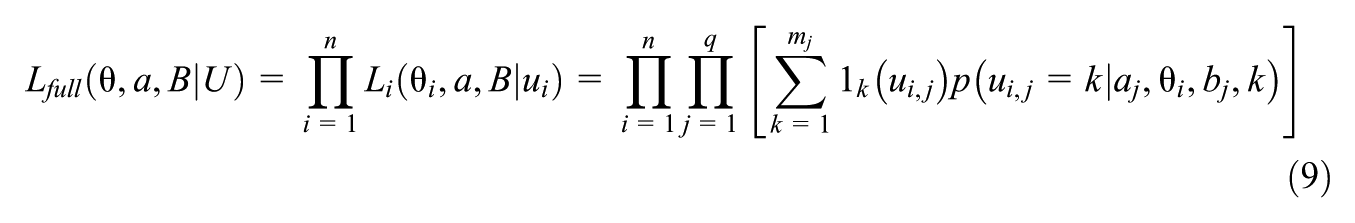
In educational testing, psychological measurement, and behavioral assessment, item response theory (IRT) models aim to infer latent traits (e.g. abilities and attitudes) of individuals from observable responses to test items. Marginal maximum likelihood (MML) is a popular frequentist estimation method in the IRT literature, treating person abilities as latent variables (random effects) and widely used in practice. However, computing the marginal likelihood requires integrating over the latent traits, leading to complex numerical integration that can become intractable for large-scale assessments or high-dimensional latent structures. To improve the computational efficiency of MML, a variety of algorithms have been proposed, such as the Metropolis–Hastings Robbins–Monro algorithm (Cai, 2010) and variational Expectation–Maximization (Jeon et al., 2017).
Bayesian IRT models (Fox, 2010) are increasingly popular because they allow flexible specification of complex models, but Bayesian estimation further increases computational demands by requiring computation of posterior distributions over parameters, typically involving integration over high-dimensional spaces. Markov Chain Monte Carlo (MCMC) algorithms, such as the Metropolis–Hastings algorithm (Hastings, 1970; Metropolis et al., 1953), are widely used to approximate these integrals, yet they can be computationally intensive and slow to converge in the high-dimensional settings typical of IRT. These challenges are exacerbated by large datasets and complex model structures (e.g. multidimensional traits), underscoring the importance of efficient gradient computation and scalable optimization for improving parameter estimation in IRT models.
1.3 DL Frameworks Improving Computational Efficiency for IRT Models
The computational strengths and flexibility of PyTorch and TensorFlow offer promising tools for addressing the computational challenges in IRT. Their support for AutoDiff reduces the need to manually derive complex gradients in likelihood functions. Using the probabilistic programming libraries Pyro and TFP, researchers can specify IRT models within these frameworks and leverage advanced inference algorithms such as HMC and VI. These algorithms are implemented efficiently, taking full advantage of AutoDiff and optimized computational kernels, which allows for faster convergence and better scalability; for example, HMC uses gradient information to explore the parameter space more effectively than traditional random-walk MCMC (Neal, 2011). VI provides another powerful numerical method, widely used for training large-scale Bayesian neural networks: it approximates the posterior by finding the closest distribution within a specified family, turning inference into an optimization problem that is generally faster and more scalable (Blei et al., 2017). Although MCMC-based estimates are often slightly more accurate at the cost of higher computation (C. Ma et al., 2024; Urban & Bauer, 2021), VI, as an optimization-based approach, can benefit substantially from GPU acceleration available in these frameworks. Moreover, because the model specification and computational backend remain largely unchanged, these frameworks provide a convenient and fair platform for comparing traditional MCMC methods with rapidly evolving VI approaches simply by swapping inference routines, thereby minimizing confounding implementation differences.
While the HMC algorithm has already been introduced on the R platform using Stan (Carpenter et al., 2017) to estimate IRT models (Y. Luo & Jiao, 2018), Python frameworks such as PyTorch and TensorFlow provide more adaptable and scalable environments for constructing sophisticated probabilistic models. Their extended libraries, including Pyro and TFP, not only facilitate the implementation of HMC and VI but also seamlessly integrate a wide range of neural network architectures. Both frameworks are under continuous development by leading DL research communities, with state-of-the-art neural network designs and learning algorithms regularly incorporated. This ongoing evolution streamlines the construction of complex, nonlinear, and hierarchical models and broadens the scope for extending IRT models beyond traditional forms, including applications that make use of multimodal data.
On the technical front, recent IRT research has begun to explore how advanced computing techniques, particularly VI and related methods, can be adapted and improved for IRT estimation (N. Luo & Ji, 2025; B. Ma et al., 2022; Urban & Bauer, 2021). However, these contributions tend to emphasize methodological innovation and are often presented in highly technical language with Python/PyTorch implementations, making them less accessible to applied researchers and psychometric practitioners. As a result, there remains a noticeable gap in practical, accessible discussions and tutorials (Y. Luo & Jiao, 2018; McClure, 2023) that explicitly bridge probabilistic machine learning, DL, and IRT models. The goal of this article is to demonstrate how DL computational platforms can be effectively employed to estimate parameters in IRT models. Our contribution is twofold: first, we provide the psychometric community with a didactic yet in-depth introduction to PyTorch and TensorFlow specifically in a psychometric context (in contrast to more general reviews such as Pang et al., 2020), while also offering computer science and machine learning researchers a tutorial on commonly used psychometric models; second, by framing IRT models through the lens of graphical models (a central framework in probabilistic machine learning) we provide intuitive discussions and visualizations that aid in understanding and interpreting complex models and encourage interdisciplinary collaboration between psychometrics and DL. This contribution is particularly timely given the rapid advances in DL and artificial intelligence and the fact that recent applications of DL in IRT are often highly technical and present a steep learning curve for researchers without prior exposure to these methods (Cho et al., 2021; Converse et al., 2021; N. Luo & Ji, 2025; C. Ma et al., 2024; Urban & Bauer, 2021). By providing step-by-step guidance and practical demonstrations within flexible DL frameworks, we aim to promote wider adoption of these advances and to foster innovative approaches in measurement and assessment.
The rest of this article is structured into five main sections to provide a comprehensive introduction and tutorial on using DL computation frameworks for fitting various IRT models. The first section briefly introduces IRT model construction and Bayesian parameter estimation. The second section provides a detailed tutorial showing how to estimate parameters in PyTorch and TensorFlow. The third and fourth sections compare the estimation performance of HMC and VI implemented in these two frameworks using various simulated and empirical datasets, respectively. The article concludes with a comprehensive discussion highlighting the strengths and limitations of DL frameworks and providing general guidance for choosing HMC and VI methods in practice.
2. Overview of IRT Models and Bayesian Analysis
This section outlines the specifications of dichotomous and polytomous item response models, specifically the graded response model (GRM) and the partial credit model (PCM). Additionally, it provides a brief introduction to Bayesian parameter estimation.
Using the observed response matrix as input data, the model estimates both item parameters and explores the latent traits of examinees through the structure of IRT. A key assumption is that examinees are independent of one another. Furthermore, given an examinee’s latent trait, their responses to different items are assumed to be independent. IRT models, with their inherent dependencies among parameters, can be viewed as special cases of probabilistic graphical models. In this context, DL frameworks have been employed to facilitate parameter estimation (Johnson et al., 2016; Paszke et al., 2017).
2.1 IRT Models
IRT models can date back to Rasch’s introduction of the Rasch model in 1960. This model has excellent statistical properties due to the natural exponential family form and has influenced how researchers think about measuring psychological traits (Rasch, 1960). Around the same time, Lord and Novick (1968) provided a general framework for IRT models and introduced the two-parameter (2PL) and three-parameter logistic (3PL) models, developed by Birnbaum (1968). These models include not only item difficulty but also how well an item can distinguish between different levels of latent trait, and for the 3PL model, the likelihood of guessing the correct answer (Birnbaum, 1968; Lord & Novick, 1968).
The IRT models mentioned above belong to the dichotomous IRT models, which deal with binary responses. IRT models can be further categorized according to the dimensions of latent traits and individual’s responses to a set of items. Later developments expanded IRT to include polytomous models to handle items with multiple categories of responses, such as questions with more than two possible answers. Important polytomous models include the GRM (Samejima, 1969), the PCM (Masters, 1982), and the nominal response model (Bock, 1972). More general and complex IRT models raise the dimension of latent traits, such as the multidimensional 2PL IRT model (Reckase, 2009).
2.1.1 Dichotomous IRT Models—Unidimensional
Model parameters for IRT usually include each examinee’s latent ability and each item’s parameters, such as discrimination, difficulty, and the pseudo-guessing parameter, which we introduce below. Dichotomous IRT models are those with a binary response, with “
where
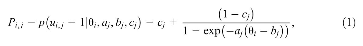
Graphical representations play a role in understanding complex latent variable models in probabilistic machine learning. These visual tools, often expressed as directed or undirected graphs, provide a structured framework that represents the probabilistic dependencies between observed data and latent variables. In probabilistic machine learning, this approach is particularly useful because it offers an intuitive illustration of how parameters, latent variables, and observations interact, rather than relying solely on abstract equations. Figure 1 illustrates the graphical model demonstrations for these IRT models. The shaded variables are the observed variables, and all dependencies between variables are shown by arrows.
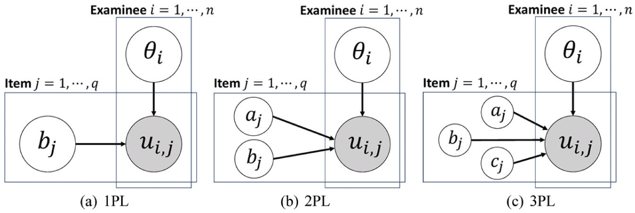
Graphical model demonstrations for the dichotomous IRT models (unidimensional case) (a) 1PL (b) 2PL (c) 3PL.
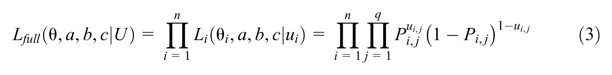
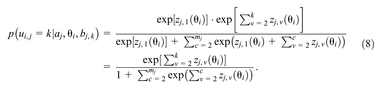
The statistical model can be summarized in the full likelihood function. Let
Let
2.1.2 Dichotomous IRT Models—Multidimensional
The examinee usually requires multiple abilities to answer a question accurately, so a more general construct is to assume the examinee’s latent ability and the item’s discrimination as a set of values rather than a single number. For instance, items for a mathematics test might depend on two skill constructs: arithmetic problem-solving and algebraic symbol manipulation. Taking the 2PL IRT model as an illustrated example, with the modification, where
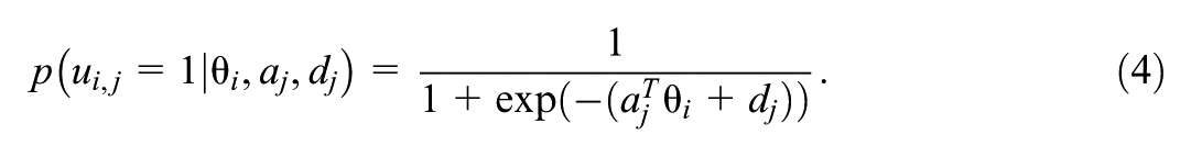
Figure 2(a) shows the graphical demonstration for the multidimensional 2PL IRT model. The full likelihood function is similar to the unidimensional case mentioned above, except that the parameters are replaced with their multivariate counterparts. Multivariate distributions and matrix multiplication should be included to extend the dimensions in the code implementation.
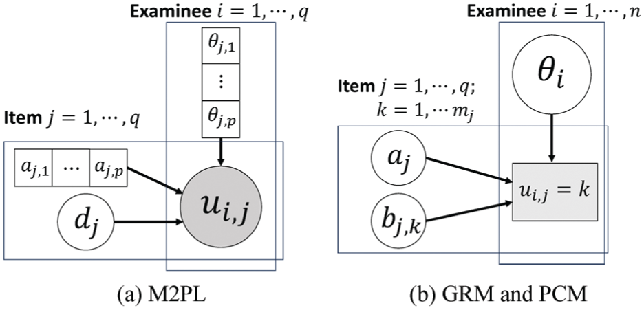
Graphical model demonstrations for the (a) multidimensional 2PL IRT model (b) GRM and PCM.
2.1.3 Polytomous Item Response Models
Polytomous item response models consider responses with more than two categories, that is, not just correct and incorrect. The GRM and the PCM are introduced below. They can be demonstrated using the same graphical model in Figure 2(b).
The GRM (Samejima, 1969), one type of the ordinal response models, is a general version of the 2PL IRT model and handles ordinal polytomous categories relating to constructed-response or selected-response items. To be specific, examinees are supposed to obtain multiple levels of ordinal scores such as
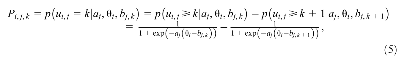
where

The PCM (Masters, 1982) is another type of ordinal response models and is constructed on the basis of items that can be partially correct. For a multicategory item
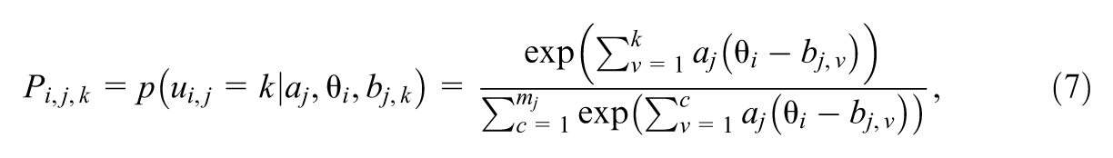
where
For GRM and PCM, the likelihoods given by the whole response matrix
where
The multidimensional extensions of GRM and PCM can be achieved by replacing the unidimensional latent ability
2.2 Bayesian Approach for Parameter Estimation
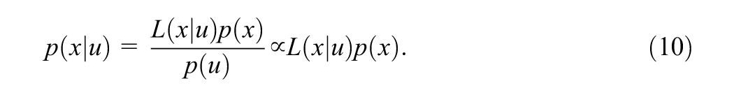
The Bayesian approach to parameter estimation provides a robust framework for incorporating prior knowledge and updating beliefs in light of new data (Patz & Junker, 1999a, 1999b). This is achieved by characterizing parameters not as fixed points, but as probability distributions. The core of this approach rests on Bayes’ theorem, which synthesizes prior beliefs about parameters
A significant computational challenge arises from the denominator,
HMC (Neal, 2011) is an advanced MCMC algorithm designed for efficient sampling from the posterior distribution. The general goal of MCMC is to construct a Markov chain whose stationary distribution is the target posterior. After a sufficient number of steps, samples drawn from this chain can be treated as samples from the posterior itself. Unlike simpler MCMC methods that employ a random walk, HMC uses gradient information from the log-posterior to guide its exploration of the parameter space, making it a highly efficient sampler (Carpenter et al., 2017). By introducing an auxiliary momentum variable and simulating Hamiltonian dynamics, HMC can propose distant, yet high-probability, new states, leading to faster convergence and less correlation between successive samples. A key challenge in standard HMC is the need to manually tune simulation parameters, particularly the number of integration steps,
Variational inference offers a different, often faster, alternative to sampling. Instead of attempting to draw samples from the true posterior

The ELBO consists of two intuitive terms. The first term, the expected log-likelihood, encourages the variational distribution to explain the observed data. The second term is the KL divergence between the variational distribution and the prior, which acts as a regularizer, penalizing deviations from our prior beliefs. By using gradient-based optimization methods to maximize the ELBO with respect to
3. Fitting IRT Models Using PyTorch and TensorFlow
This section provides a detailed explanation for the code snippets in Supplementary Appendix (available in the online version of this article) with respect to the implementation of the IRT model construction and parameter estimation in two DL frameworks. We use PyTorch and TensorFlow, as well as their probabilistic programming libraries extensions, Pyro and TFP, to build statistical models and perform inference from scratch. Table 1 summarizes the key input requirements for configuring HMC and VI.
Input Summary for HMC and VI Configuration in PyTorch and TensorFlow
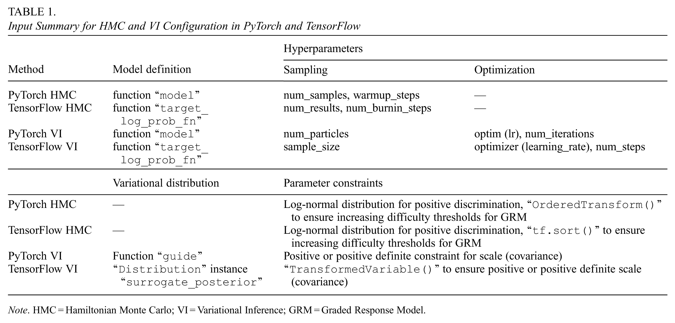
Note. HMC = Hamiltonian Monte Carlo; VI = Variational Inference; GRM = Graded Response Model.
3.1 Unidimensional 3PL IRT Model
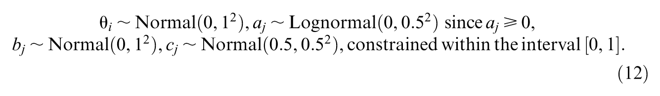
A step-by-step illustration is first presented for the unidimensional 3PL IRT model. For IRT models, parameters can be sampled from specific distributions once the hyperparameters for distributions, like the mean and variance of the distributions, are set. For instance, we adopt weakly informative priors distributions of examinees’ ability
Examples of how to set up distributions like the Equation 12 and start sampling are presented first in codes 1 and 2. Also, in order to perform a simulation study in the next section, these are also the first step, showing how to sample true parameters for the evaluation of parameter estimation and to simulate a response matrix based on the true parameters and the Equation 1. Although examinees’ ability and items’ parameters have different shapes, in PyTorch and TensorFlow, broadcasting allows tensors with different shapes to be automatically expanded to have compatible dimensions for elementwise operations and does not need explicit replication of data (Code 1, line 30; Code 2, line 31). This feature simplifies operations on tensors of varying sizes, enabling more efficient and concise code for computations such as addition, multiplication, and other arithmetic operations.
3.1.1 HMC Setting
After setting the prior distributions, the next step is to compute the likelihood function as the statistical model according to Equation 3. This requires the probability computation of the response matrix
The instantiation of NUTS in Pyro requires defining a probabilistic model (“
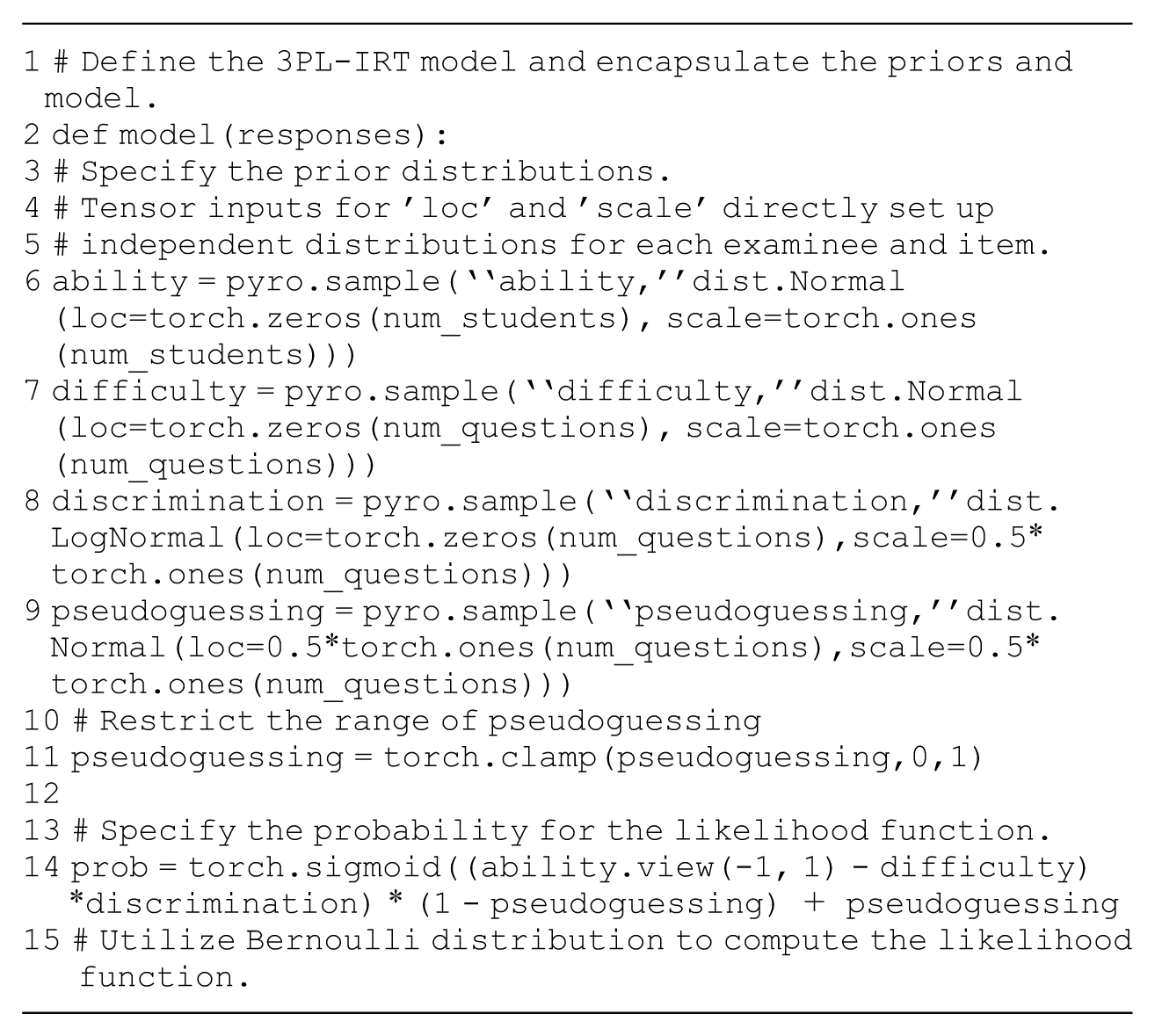
The argument “
3.1.2 VI Setting
Pyro provides built-in modules for doing variational inference in the class “
TFP also has a module “
3.2 Multidimensional 2PL IRT Model
The multidimensional extension of IRT models increases the complexity of computation. For instance, it is assumed that the examinee might require two types of abilities to give the correct answers for the items. Therefore, for each examinee, the dimension of the ability parameter is 2, and for each item, the discrimination parameter also has two dimensions. With mean vector
a priori independent distributions for examinees’ latent abilities and items’ discrimination and difficulty are set as follows: for

The likelihood function is computed according to Equation 4.
For HMC, the only difference in code implementation compared to the 3PL IRT model is the inclusion of priors and the model. The code snippets for setting up the “
3.3 Graded Response Model
The GRM assumes that each item can have multiple ordinal response categories, with each category representing an increasing level of difficulty. As a result, a multivariate distribution should be applied to the difficulty parameters to properly capture these levels. For example, if the GRM defines three ordinal score levels for each item, the vector of difficulty parameters for item
Given the constraint shown in Equation 6, only a subset of the difficulty parameters needs to be modeled. Specifically, they can be sampled from a two-dimensional multivariate normal distribution with mean vector

The likelihood function is set up as the statistical model according to Equations 5 and 9. The code snippet for the encapsulation of the prior distributions and likelihood function is presented in Codes 10 and 11. Similarly to the previous two models, for VI in PyTorch, the “
3.4 Partial Credit Model
The PCM also assumes multiple response categories for each item but removes the requirement for increasing difficulty parameters across categories. We consider a test of 10 items with
The prior distributions for the parameters can be set following Equations 12 or 15. The computation of the likelihood function is guided by Equations 8 and 9. A Python dictionary can be used to store and organize the structure of the tests and the sizes of their components. Codes 13 and 14 for implementing HMC sampling are shown in Supplementary Appendix (available in the online version of this article). For VI in PyTorch, again, only the variational distribution part should be modified as shown in Code 15.
4. Simulation Studies
4.1 Basic Comparision Based on Different IRT Models
This section presents the results of simulation studies using the HMC and VI methods introduced in the previous section. Four models are taken as examples: the unidimensional and multidimensional 2PL IRT models, GRM, and PCM. As this article serves as a tutorial, relatively simple cases with small sample sizes and small numbers of dimensions and repetitions are considered. All experiments were conducted using Google Colab, a cloud-based platform providing free access to computational resources. The experiments ran on a standard Colab environment with a virtual machine powered by a 12GB of RAM and a single-core CPU.
Across all studies, we fix
For the remaining studies, we follow a common protocol: priors follow each model’s assumptions in its subsection, we generate 100 response matrixes, and estimate with HMC and VI using the listed code (i.e. Multidimensional 2PL in Section 3.2: Codes 7, 8, 9; GRM in Section 3.3: Codes 10, 11, 12; PCM in Section 3.4: Codes 13, 14, 15). The estimation repeated 100 times for each model.
4.1.1 Evaluation Criteria
Simulated data are randomly generated, so the repetition of the process across simulated data sets provides insights into the stability and robustness of the performance. In order to evaluate the performance of the estimation process, mean square error (MSE) and bias are often calculated for each parameter. The MSE directly quantifies how different the estimates are from the true values, and the bias reflects whether or how the estimates skew off from the true values.
For a true parameter

where
The results based on 100 simulated response matrixes can be considered as 100 Monte Carlo samples of estimates. The mean value is a point estimate of the true MSE using Monte Carlo estimation. Since the number of simulations is not large, Monte Carlo Standard Error (MCSE) is required to approximate the estimation noise and quantify how large the uncertainty is in the estimate of quantities such as MSE and bias (Koehler et al., 2009). The slight MCSE in the experiments supports, for the purpose of this tutorial, that it is sufficient to show the DL frameworks’ effectiveness with 100 simulated datasets. Different MSEs across the 100 simulated response matrixes are further summarized by calculating the mean and MCSE across replications:


Bias also assesses a model’s ability to capture the underlying patterns in the data, and a bias value close to 0 indicates unbiased parameter estimation without skew. Again, for instance, with
The MCSE of bias across replications can also be obtained as

For high-dimensional parameters, the definitions of MSE and bias must be slightly modified. For example, considering the true parameters
and the bias of discrimination parameters across items is defined by removing the square in Equation 21, similar to the first study.
4.1.2 Results
For the HMC method, as an extension of the MCMC method, a trace plot can evaluate whether the sampler sufficiently explores the parameter space without accepting or rejecting excessive proposals and check the convergence state. The trace plot is shown in Figure A1 in Supplementary Appendix (available in the online version of this article). The values change at an acceptable frequency and within a small range, indicating HMC has adequately explored the space of parameters and achieved convergence.
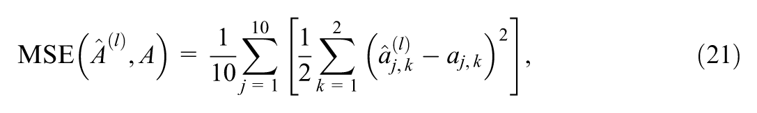
To assess bias and MSE, the mean and MCSE of MSE and bias of estimated difficulties and discrimination throughout 100 simulated response matrices are calculated as shown in Figure 3. For the HMC method, the performances in PyTorch and TensorFlow do not have an obvious difference. The estimates of parameters using HMC and VI approaches are accurate according to the fairly low MSE. The low bias indicates that MCMC inference and variational inference efficiently capture the underlying patterns in the data. The MCSE values are all small, indicating that the estimates of MSE and bias are stable across replications so 100 repetitions are sufficient to ensure the effectiveness of DL frameworks.
MSE and bias of estimated parameters throughout 100 simulated response matrixes (a) MSE (b) Bias.
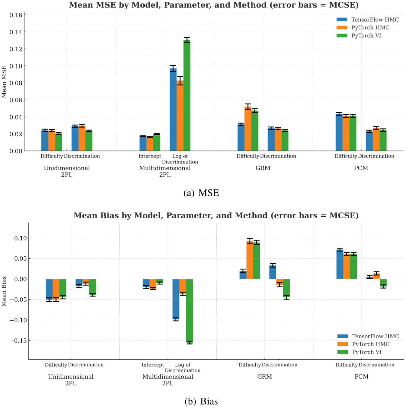
To evaluate the computational efficiency, the computation time for each simulation study is recorded, and the plot of computation times for the four simulation studies is summarized in Figure 4. VI is generally faster than HMC, especially for more complex models. The computation time for PyTorch and TensorFlow is similar, except for the multidimensional 2PL model, where TensorFlow outperforms PyTorch and is even faster than the TensorFlow codes in the first study.
Computation time by model types and methods.
4.2 Simulation Study: Prior Sensitivity Analysis
This section presents a simulation study to evaluate the prior sensitivity of HMC and VI for the 2PL IRT model. Prior sensitivity analysis is crucial in Bayesian statistics, as it helps assess how different prior choices influence posterior estimates. This is particularly important in IRT applications with small item pools, where the amount of information available from the data may be limited, making the choice of priors more impactful.
We generate a 2PL IRT dataset with
The prior sensitivity analysis is designed to reflect a practical situation in which the analyst may be unsure about how strongly to regularize item parameters when the number of items is small. Hence, we vary the scale of the priors for discrimination and difficulty while holding the ability prior constant:
For HMC with NUTS, we use the implementation in Pyro, with 400 posterior samples following 300 warm-up iterations, one chain. For variational inference, we use SVI in Pyro with learning rate 0.03, 4,000 iterations; posterior summaries are obtained from 1,000 draws from the variational approximation. These settings are chosen to keep the two approaches comparable in computational budget while reflecting typical default choices for small-scale IRT applications.
Figure 5 shows the MSE results, and Figure A2 in the Appendix (available in the online version of this article) shows the bias results. Both methods recover difficulty reasonably well across prior scales, with biases close to zero and MSEs mostly between 0.028 and 0.056. The smallest difficulty prior scale (0.5) produces slight positive bias in
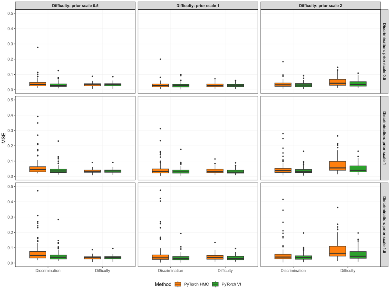
Discrimination and difficulty MSE across prior scale combinations for HMC and VI.
The more pronounced differences between methods arise for discrimination. When the discrimination prior is tight (scale 0.5), both methods show small positive bias in
Taken together, these findings suggest that, under the present design with a short test and moderate sample size, VI provides more robust discrimination recovery to plausible prior-scale choices, while both methods are broadly comparable for difficulty. The elevated and unstable discrimination MSE under HMC with larger discrimination scales likely reflects the combination of weaker regularization and limited item information, which can make the posterior geometry harder to explore efficiently with the current sampling budget (one chain and 400 retained draws). In this setting, a moderate prior scale for item parameters (around 1) appears to offer a sensible trade-off between shrinkage and flexibility, yielding small bias and relatively low MSE for both approaches. However, VI’s apparent robustness to prior-scale variation may be partly driven by its tendency to concentrate mass in high-density regions of the posterior, thereby dampening the influence of weaker priors in the tails of the parameter space.
4.3 Simulation Study: Large-Scale Assessment
This section evaluates method performance in a setting that is closer to the scale of many contemporary testing programs. When the number of items and examinees increases, computational efficiency and numerical stability become central practical concerns, even for conceptually standard unidimensional IRT models. A large-response design therefore provides an appropriate benchmark for assessing whether DL platform-based implementations deliver reliable inference while maintaining feasible runtime in realistic, high-information applications.
We conduct a large-scale simulation under a unidimensional 2PL IRT model with
For three estimation approaches: TensorFlow HMC, PyTorch HMC, and PyTorch SVI, we set weakly informative priors:
Across replications, the MSE and bias of discrimination and difficulty parameters, along with computation time for each method, are summarized in Figure 6. All three methods achieve very small estimation error for both discrimination and difficulty. The MSE distributions in the accompanying boxplots are tightly concentrated, indicating stable recovery in this high-information setting. The two HMC implementations yield nearly identical accuracy, with difficulty MSE around 0.0027 (Standard deviation [SD] ≈ 0.0005) and discrimination MSE around 0.0021 (SD ≈ 0.0003). The VI approach matches HMC for discrimination MSE at approximately 0.0021 (SD ≈ 0.0003) and shows only a marginal increase for difficulty, around 0.0028 (SD ≈ 0.0005). Bias patterns are similarly close across methods for difficulty, with small positive bias of roughly 0.015 for all three approaches. For discrimination, the two HMC approaches show small positive bias (about 0.0067–0.0068 with SD ≈ 0.0050), whereas VI shows a small negative bias of similar magnitude (about
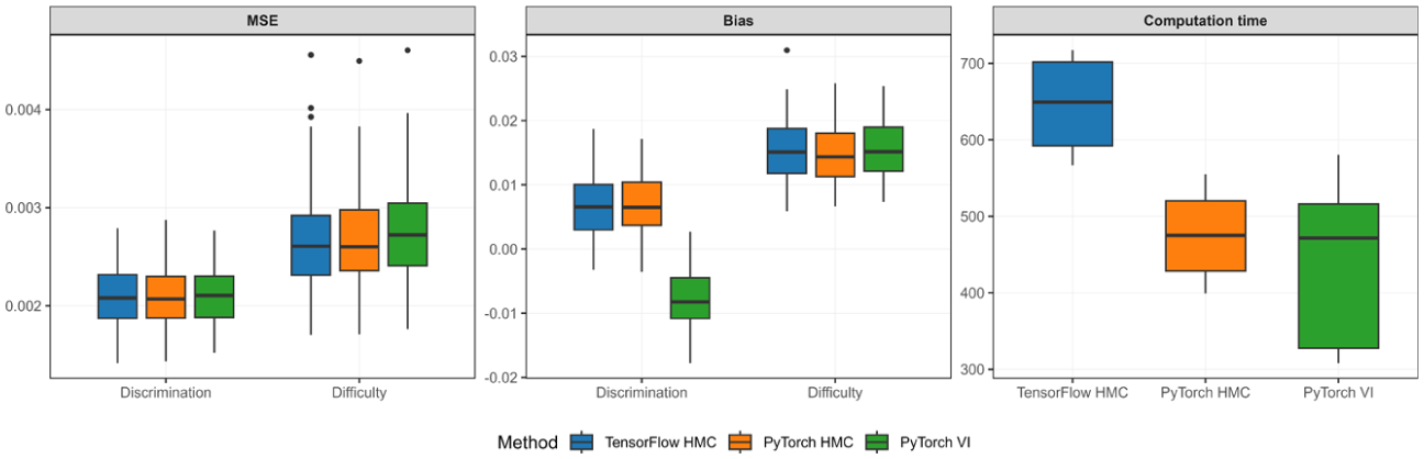
MSE and bias of discrimination and difficulty parameters in a large-scale 2PL IRT simulation, along with computation time across three methods.
The most visible contrast lies in computation time. The TensorFlow HMC implementation requires the longest runtime, averaging about 647 s (SD ≈ 56). The PyTorch HMC implementation runs substantially faster, averaging about 475 s (SD ≈ 50), while maintaining the same level of accuracy. PyTorch VI achieves the shortest average runtime at roughly 422 s, although its variability is larger (SD ≈ 94), which is also reflected in the wider spread of the time boxplot. Overall, the results indicate that when the number of items and examinees increases to a scale that is common in large educational assessments, the PyTorch-based implementations retain accuracy comparable to a TensorFlow HMC benchmark while offering clear computational advantages, and VI provides an additional speed gain with only minor, directionally interpretable differences in discrimination bias.
4.4 Simulation Study: High-Dimensional Latent Traits
This section examines a multidimensional setting in which the latent structure is substantially richer than in standard unidimensional designs. As the number of traits increases, the parameter space expands rapidly and inference must recover both item parameters and the dependence structure among abilities. Evaluating performance in a seven-dimensional model therefore helps clarify whether deep learning platform-based implementations remain accurate and efficient when the latent space is relatively large.
We simulate responses under a confirmatory M2PL model with
We compare PyTorch HMC and PyTorch VI under priors that mirror the data-generating structure. We place an Lewandowski-Kurowicka-Joe (LKJ) prior on the ability correlation matrix via
Figure 7 summarizes the MSE and bias of ability correlation, item difficulty, and discrimination parameters, along with computation time for each method across the 100 replications. The results show that both methods recover the key components of the model with small errors despite the seven-dimensional latent space. For the ability correlation parameters, HMC produces essentially unbiased estimates on average (bias
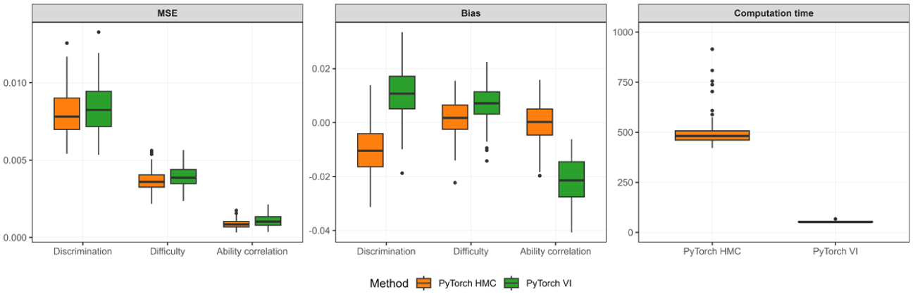
MSE and bias of discrimination, difficulty, and ability correlation parameters in a confirmatory M2PL IRT simulation, along with computation time across two methods.
Computation time separates the two approaches most clearly. HMC requires substantially longer runtime on average (about 588 s) and shows high variability across replications (SD
5. Empirical Study
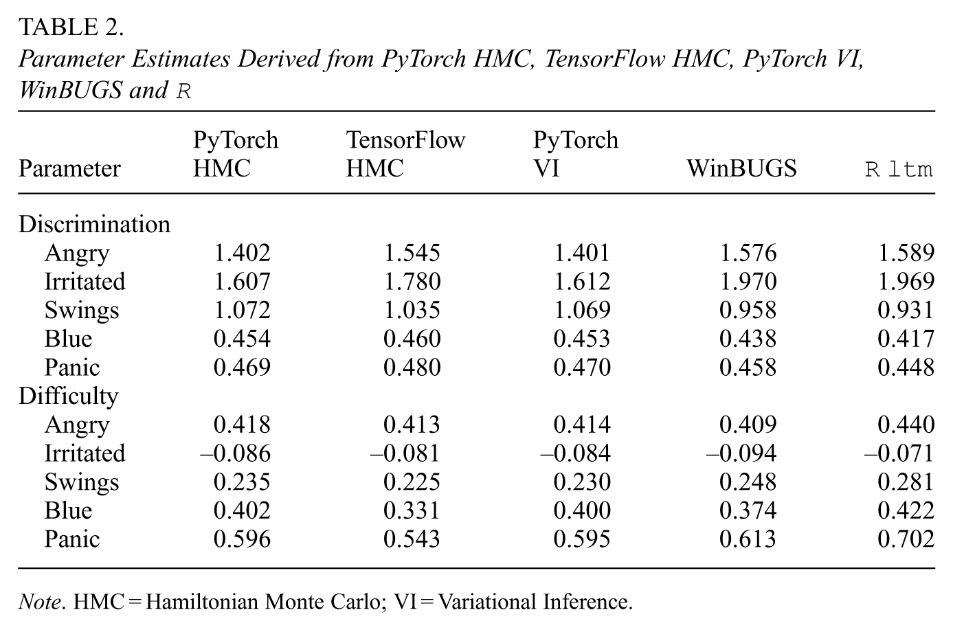
This section details an empirical investigation utilizing the “bfi” dataset from the psychpackage in R (Revelle, 2024) to illustrate parameter estimation for the PCM using both PyTorch and TensorFlow. The findings are further contrasted with estimates obtained from WinBUGS and R’s package ltm, as reported by Li and Baser (2012). The “bfi” dataset comprises responses from 2,800 subjects to 25 personality self-report items, corresponding to the five hypothesized dimensions of personality, namely the Big Five traits (Goldberg, 1992). In this study, our focus is confined to the five items that assess neuroticism, a trait defined by a predisposition to experience negative emotions. These items evaluate tendencies such as anger (e.g. “Get angry easily”), irritation and mood instability (e.g. “Get irritated easily” and “Have frequent mood swings”), depression (e.g. “Often feel blue”), and anxiety (e.g. “Panic easily”).
Each item is rated on a six-point scale, ranging from “1. Very inaccurate” to “6. Very accurate.” In the context of IRT, these response categories function as indicators of the latent construct of neuroticism, with higher cumulative scores signifying greater severity of the trait. Unlike conventional summary scores, IRT modeling permits a more refined interpretation by accounting for each item’s severity threshold (i.e. the difficulty
For illustrative purposes, we present the discrimination estimates for all items and the difficulty estimates for the first item as representative examples of our parameter estimation outcomes. In the absence of definitive “true” parameter values, we compared the posterior distributions derived from PyTorch HMC, TensorFlow HMC, and PyTorch VI. As shown in Figure 8, the posterior distributions produced by these methods are highly congruent.
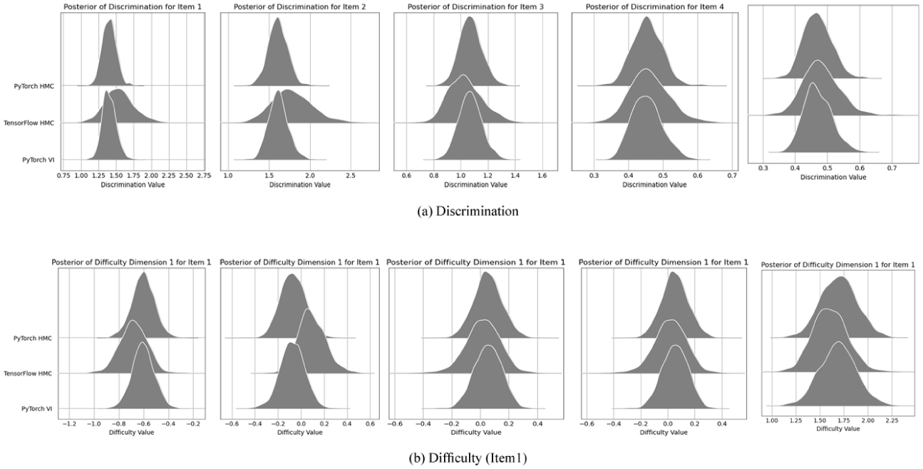
Posterior distributions derived from PyTorch HMC, TensorFlow HMC, and PyTorch VI (a) Discrimination (b) Difficulty (Item 1).
Furthermore, for each neuroticism item, we compute the posterior mean as the point estimate. For simplicity, the average difficulty estimates across the response thresholds are calculated as
Parameter Estimates Derived from PyTorch HMC, TensorFlow HMC, PyTorch VI, WinBUGS and
Note. HMC = Hamiltonian Monte Carlo; VI = Variational Inference.
Two more empirical studies are presented in Supplementary Appendix (available in the online version of this article) to further illustrate the application of the DL framework in practice. One study analyzes an educational assessment dataset to illustrate the practical use of the GRM implemented in PyTorch and compares the results with those from R’s package
6. Discussion
DL offers powerful tools for modeling complex relations in data, especially when leveraging highly expressive models and large datasets. PyTorch and TensorFlow, together with their probabilistic ecosystems (e.g. Pyro and TFP), provide flexible and scalable environments for statistical modeling, including IRT models.
In this article, we provided a detailed introduction to using PyTorch and TensorFlow to fit common IRT models. Our simulation studies demonstrate excellent estimation performance, with low MSEs and biases for model parameters. Both the MCMC method using NUTS and the direct application of VI efficiently estimate model parameters. A prior sensitivity analysis further illustrated that HMC method might be more sensitive to choices of prior scales than VI in moderate-scale assessments. Two large-scale simulation studies showcased the scalability of these frameworks for unidimensional and multidimensional IRT models. Three empirical study further illustrated how these two frameworks function in practice.
Two notable observations emerged. First, regarding user-friendliness, PyTorch and TensorFlow differ in practice. Based on the length of code snippets and the complexity of code design, especially for VI implementations, PyTorch appears to offer a more accessible interface, likely aided by its rich set of predefined functions. This aligns with evidence from broader comparisons of the two ecosystems (Novac et al., 2022). Second, our analysis indicates that VI is substantially faster than MCMC, particularly for large-scale or high-dimensional models, while maintaining comparable accuracy in parameter recovery. However, it is important to recognize VI’s well-documented tendency to concentrate posterior mass in regions of high density and underestimate posterior variances (Blei et al., 2017), a pattern that is reflected in our results through weaker sensitivity to the prior scale in the prior sensitivity analysis and a negative bias in the recovery of ability correlations in the high-dimensional M2PL simulation. In psychometrics, related concerns and potential remedies have been discussed for multidimensional IRT and extensions of Gaussian VI (Cho et al., 2021; C. Ma et al., 2024). Therefore, VI should be used with caution when the primary goal is statistical inference rather than point estimation. In general, for practitioners prioritizing computational efficiency and scalability, VI presents a compelling option, whereas MCMC remains a robust choice when accurate uncertainty quantification is essential.
Although we did not empirically compare our implementations to dominant psychometric software (e.g. flexMIRT or ConQuest Adams et al., 2020; Chung & Houts, 2020) or to alternative highly optimized methods for large-scale or complex IRT models, adopting these DL frameworks remains meaningful. A key reason is that the AutoDiff tools in PyTorch and TensorFlow play a crucial role in efficiently computing gradients, facilitating algorithms that require derivative computations, such as HMC. These tools are not restricted to fully Bayesian analyses with priors on all parameters. The same computational infrastructure can support frequentist IRT estimation approaches, including MML-type objectives and joint maximum likelihood-style optimization. For example, Gaussian variational EM provides an efficient likelihood-based alternative for MIRT calibration in a frequentist spirit (Cho et al., 2021), and recent work has used neural architectures to amortize JMLE for item factor models (Molenaar et al., 2025). Related large-scale JML developments in psychometrics also highlight how optimization-based approaches can be competitive when dimensionality is high (Chen et al., 2019). In addition, VI objectives in these frameworks are differentiable and can, in principle, benefit from modern accelerators (e.g. GPUs), which further motivates learning and adopting this computational environment.
More broadly, leveraging DL frameworks not only enables efficient computation but also opens opportunities to integrate neural network architectures into IRT modeling. This integration may help capture complex, nonlinear relationships and better handle diverse data modalities, potentially expanding the scope of traditional IRT. Specifically, the likelihood function or parameter probability density can be modeled with flexible neural modules (Cho et al., 2021; Liu et al., 2022; Urban & Bauer, 2021). Advanced architectures such as convolutional neural networks (LeCun et al., 1990) and long short-term memory networks (Hochreiter & Schmidhuber, 1997) offer a natural way to represent structured inputs that extend beyond traditional item formats. This flexibility has the potential to enrich the IRT literature by enabling principled modeling of multimodal data within a unified estimation framework.
The fusion of IRT and DL also offers a practical path for handling models with a large number of parameters and complex input representations, with clear value when multimodal information is tied to explicit measurement targets. Rather than displacing response data, multimodal inputs can be used to derive or augment psychometrically meaningful variables that enter familiar IRT structures. For example, IRT models informed by item text or format demonstrate how auxiliary representations can improve measurement and interpretation (B. Ma et al., 2022; Cheng et al., 2019). A concrete multimodal use case is spoken language proficiency: examinee audio responses can be processed by neural models to extract substantively aligned features (e.g. fluency, pronunciation, prosody) or to map responses into rubric-based categorical scores, which can then be calibrated as polytomous items or incorporated as predictors in explanatory IRT frameworks. This provides explicit grounding in the psychometric goal of improving measurement of speaking ability while retaining the interpretability of IRT. Related work evaluating automated speech assessment systems with IRT-based fairness and bias analyses further indicates a realistic pathway for integrating audio-derived evidence into operational measurement (Kwako et al., 2022). Similar strategies could be extended to other modalities (e.g. image-based tasks, sentiment-informed textual feedback, or physiological signals) when those data streams are conceptually linked to well-defined constructs and scoring rubrics in assessment contexts.
We hope this article assists researchers in understanding and conceptualizing Bayesian IRT analysis using powerful DL computing frameworks. While HMC and VI have been increasingly discussed in the IRT literature, we provide an accessible introduction and concrete code examples for common dichotomous and polytomous IRT models, alongside a practical comparison of the two dominant DL platforms. This foundation may help readers engage with recent advances in Bayesian estimation using modern VI variants and neural-enhanced IRT approaches (Cho et al., 2021; Liu et al., 2022; C. Ma et al., 2024; Urban & Bauer, 2021).
Despite the promise of integrating IRT with DL frameworks, several challenges and limitations remain. Incorporating techniques from other fields into traditional IRT requires reconciling differences in methodology, data structures, and analytical conventions, often demanding substantial effort and specialized knowledge. Moreover, the inherent complexity of DL models can reduce interpretability, a critical concern in educational and psychological assessment where transparency is essential. Finally, our study does not provide a direct empirical comparison of parameter accuracy or computational efficiency against conventional estimation methods (e.g. MMLE) implemented in established IRT software such as flexMIRT or ConQuest (Adams et al., 2020; Chung & Houts, 2020). We leave these comparisons for future research.
Supplemental Material
sj-pdf-1-jeb-10.3102_10769986261439301 – Supplemental material for Fitting Bayesian Item Response Theory Models Using Deep Learning Computational Frameworks
Supplemental material, sj-pdf-1-jeb-10.3102_10769986261439301 for Fitting Bayesian Item Response Theory Models Using Deep Learning Computational Frameworks by Nanyu Luo, Yuting Han, Jinbo He, Xiaoya Zhang and Feng Ji in Journal of Educational and Behavioral Statistics
Footnotes
Declaration of Conflicting Interests
The authors declared no potential conflicts of interest with respect to the research, authorship, and/or publication of this article.
Funding
The authors disclosed receipt of the following financial support for the research, authorship, and/or publication of this article: Feng Ji was supported by the Seed Grant of the International Network of Educational Institutes (Grant Number 522011), the Connaught Fund (Grant Number 520245), and the Social Sciences and Humanities Research Council (SSHRC) of Canada (Grant Number 215119, Canada Research Chair: CRC-2024-00169).
Notes
Authors
NANYU LUO is a PhD candidate in the Department of Applied Psychology and Human Development at the University of Toronto, Toronto, ON M5S 1V6, Canada; email:
YUTING HAN is a lecturer in the Cognitive Science and Allied Health School at Beijing Language and Culture University, Beijing 100083, China; email:
JINBO HE is an associate professor in the Department of Biosciences and Bioinformatics at the School of Science, Xi’an Jiaotong-Liverpool University, Suzhou, Jiangsu 215123, China; email:
XIAOYA ZHANG is an assistant professor in the Department of Family, Youth and Community Sciences at the University of Florida, Gainesville, FL 32611, USA; email:
FENG JI is an assistant professor in the Department of Applied Psychology and Human Development, at University of Toronto, Toronto, ON M5S 1A1, Canada; email:
References
Supplementary Material
Please find the following supplemental material available below.
For Open Access articles published under a Creative Commons License, all supplemental material carries the same license as the article it is associated with.
For non-Open Access articles published, all supplemental material carries a non-exclusive license, and permission requests for re-use of supplemental material or any part of supplemental material shall be sent directly to the copyright owner as specified in the copyright notice associated with the article.