Valid Standard Errors for Bayesian Quantile Regression With Clustered and Independent Data

Abstract

Bayesian quantile regression typically uses the asymmetric Laplace distribution as working likelihood, not because it is a plausible data-generating distribution but because the corresponding maximum likelihood estimator is identical to the classical estimator by Koenker and Bassett. While point estimation is consistent, credible intervals tend to have poor frequentist coverage. We propose using infinitesimal jackknife (IJ) standard errors introduced by Giordano and Broderick, which do not require resampling and can be obtained from a single Markov chain Monte Carlo run. Simulations and applications to real data show that IJ standard errors have good frequentist properties for both independent and clustered data. We provide an R package, IJSE, that computes IJ standard errors after estimation of any model with the brms wrapper for Stan.

1. Introduction

Bayesian inference is usually based on a parametric likelihood and therefore relies on distributional assumptions. While the same kinds of likelihoods are used for point estimation in frequentist contexts, it is common practice to obtain resampling-based or robust standard errors that have good frequentist properties when the assumptions are violated. Unfortunately, resampling methods are generally not feasible in Bayesian contexts because they would require repeated computationally expensive Markov chain Monte Carlo (MCMC) runs. The Bayesian infinitesimal jackknife (IJ) introduced by Giordano and Broderick (2024) offers an appealing alternative. It yields standard errors that, like resampling standard errors, are robust against model misspecification, and it requires only a single MCMC run. In this paper, we show that IJ standard errors are a good choice for Bayesian quantile regression based on the asymmetric Laplace (AL) likelihood, because the AL likelihood is known to be misspecified.

Quantile regression is used across a wide range of fields to estimate the linear relationship between predictors and the median, 90th percentile, or other quantiles of the conditional outcome distribution. Applications of quantile regression in education and psychology include investigating whether the relationship between reading-related skills, such as vocabulary, and reading comprehension is stronger at the lower or higher ends, or in the middle, of the reading comprehension distribution (Logan, 2017; Tighe & Schatschneider, 2016), and similarly for the relationship between number line estimation skills and mathematical reasoning (Ruiz et al., 2024), and the relationship between risk factors and suicidal ideation (Rogers & Joiner, 2018). Studies that can inform education policy and practice have estimated the effect on different parts of the achievement distribution of attending public versus private schools (Furno, 2011), of interim classroom assessments (Konstantopoulos et al., 2019), and of mathematics interventions (Thompson et al., 2024). Quantile regression is also used for the educational accountability systems of 23 states (Mills, 2025) to produce student growth percentiles that place students within the current year’s test score distribution, conditional on their previous year’s test scores (Betebenner, 2009; Castellano & Ho, 2013). An advantage of this approach over alternatives is that it does not require a common (vertically scaled) assessment across grade levels.

In frequentist quantile regression, point estimates can be obtained by minimizing an appropriate loss function through linear programming algorithms (Koenker & Bassett, 1978). Unlike this classic approach, Bayesian quantile regression requires a likelihood. There are several proposals including nonparametric likelihoods (Kottas & Krnjajić, 2009; Reich et al., 2010) and empirical likelihoods (Otsu, 2008; Yang & He, 2012). However, by far the most commonly applied likelihood is the AL likelihood first employed by K. Yu and Moyeed (2001). The motivation for using an AL likelihood is that maximizing this likelihood corresponds to minimizing the loss function. The general approach of constructing a posterior through a loss function is discussed by, for instance, Syring and Martin (2019).

The AL likelihood can be thought of as a working likelihood designed to produce consistent point estimates (Sriram et al., 2013). There is no particular reason to believe that the AL distribution is the data-generating distribution or that posterior intervals based on a misspecified AL distribution have correct Bayesian or frequentist properties. Unfortunately, this problem does not appear to be well-known, and AL-based Bayesian quantile regression with model-based posterior credible intervals, as implemented in the popular R package brms (Bürkner, 2017) and Stata’s Bayesian quantile regression command (StataCorp, 2023b), is still widely used without any adjustment (Betz et al., 2022; Forthmann & Dumas, 2022; He et al., 2022; McIsaac et al., 2023; Taheri et al., 2021).

The AL likelihood has a scale parameter that effectively “weights the information in the data relative to that in the prior” (Syring & Martin, 2019) and therefore determines the spread of the posterior and the width of credible intervals (Sriram, 2015; Syring & Martin, 2019; Yang et al., 2016). This scale parameter is often set to an arbitrary constant in AL-based Bayesian quantile regression, resulting in posterior standard deviations that are misleading. Yang et al. (2016) therefore propose an adjustment to the posterior covariance matrix designed to produce correct asymptotic coverage of normal-approximation-based credible intervals (see also Sriram, 2015, for a similar approach). From now on, we will refer to posterior standard deviations as standard errors to emphasize the requirement for correct frequentist properties. Yang et al. (2016) show that their adjusted standard errors are asymptotically invariant to the scale parameter. However, we show that the adjustment is sensitive to the scale parameter when the sample size is small to moderate. Fortunately, the finite-sample frequentist performance of the adjusted standard errors seems to be satisfactory when the scale parameter is set to its maximum likelihood (ML) estimate for quantile regression at the median, as suggested by Yang et al. (2016).

In frequentist inference for quantile regression, it is common practice to use bootstrap or jackknife procedures for standard errors (Bose & Chatterjee, 2003; Koenker, 2021; Portnoy, 2014). These resampling procedures begin by producing many replicate datasets from the original dataset (e.g., by sampling units with replacement for the nonparametric bootstrap) and computing point estimates for each of these replicates. Adopting these procedures for Bayesian estimates is computationally intensive because it requires performing MCMC estimation in each replicate dataset. We therefore propose using IJ standard errors that can be viewed as approximating resampling standard errors. IJ standard errors can be obtained from a single MCMC run if log-likelihood contributions from the units are computed for each post-warmup iteration. We also propose a version of the IJ standard errors for clustered data. Simulations and applications to real data show that the IJ standard errors have good frequentist properties, both for independent and clustered data, and that posterior intervals have good coverage, especially when the AL scale parameter is estimated instead of fixed to an arbitrary constant. Although Giordano provided an R package StanSensitivity that can calculate IJ standard errors, its usage is mainly in the context of sensitivity analysis. Hence, we provide an R package, IJSE, focused on computing IJ standard errors for clustered or independent data after estimation of any model with the brms wrapper (Bürkner, 2017) for Stan (Carpenter et al., 2017).

The structure of this paper is as follows. In Section 2, we introduce AL-based Bayesian quantile regression and the adjusted standard errors proposed by Yang et al. (2016). In Section 3, we briefly motivate and define the IJ standard errors by Giordano (2020) and Giordano and Broderick (2024) and show how they can be modified to handle clustered data. For independent (non-clustered) data, Section 4 presents simulation results for IJ standard errors, model-based standard errors, and adjusted standard errors by Yang et al. (2016) when the scale parameter is fixed at a range of different values, as well as Bayesian posterior standard deviations and IJ standard errors when the scale parameter is estimated. In Section 5, we evaluate the IJ standard errors for the clustered case. The different types of standard errors are compared using real data in Section 6, followed by a brief discussion in Section 7.

2. AL-Based Bayesian Quantile Regression and Adjusted Standard Errors

2.1. The AL Likelihood

In quantile regression (Koenker & Bassett, 1978), models are specified directly for the conditional quantiles $Q_{\mathrm{\tau }}(y|x)$ of the response variable $y$ given a set of covariates $x$ , where $\mathrm{\tau }$ is the quantile level. Although the methods discussed here apply more generally, we will consider a linear quantile regression model,

$$Q_{\mathrm{\tau }}(y|x)=x^{\prime }\mathrm{\beta }\left(\mathrm{\tau }\right),$$

where $\mathrm{\beta }\left(\mathrm{\tau }\right)$ is a vector of regression coefficients for quantile level $\mathrm{\tau }$ . Interest often centers on estimating the coefficient of a covariate (or several covariates) at different quantile levels, thereby relaxing the assumption of parallel quantile lines (or hyperplanes) made in a linear regression model with a homoscedastic, normally distributed error term.

In the original frequentist setup, the point estimates are obtained as numerical solutions to the minimization problem

$$\hat{\mathrm{\beta }}\left(\mathrm{\tau }\right)={\mathrm{argmin}}_{\mathrm{\beta }\left(\mathrm{\tau }\right)}\sum _{i=1}^n{\mathrm{\rho }}_{\mathrm{\tau }}(y_i-x_i^{\prime }\mathrm{\beta }\left(\mathrm{\tau }\right)),$$

where ${\mathrm{\rho }}_{\mathrm{\tau }}(·)$ , often called the “check function” for its shape, is defined as

$${\mathrm{\rho }}_{\mathrm{\tau }}\left(u\right)=u\{\mathrm{\tau }-I(u<0)\}=\{\begin{array}{c}u\mathrm{\tau }\mathrm{if}u\ge 0\hfill \\ \multicolumn{1}{c}{-u(1-\mathrm{\tau })\mathrm{if}u<0.}\end{array}$$

Bayesian inference requires a likelihood, and K. Yu and Moyeed (2001) suggested specifying the AL distribution,

$$f_{\mathrm{ALD}}(y_i|{\mathrm{\mu }}_i,\mathrm{\sigma },\mathrm{\tau })=\frac{\mathrm{\tau }(1-\mathrm{\tau })}{\mathrm{\sigma }}\exp \{-{\mathrm{\rho }}_{\mathrm{\tau }}\left(\frac{y_i-{\mathrm{\mu }}_i}{\mathrm{\sigma }}\right)\},$$

where ${\mathrm{\mu }}_i=x_i^{\prime }\mathrm{\beta }\left(\mathrm{\tau }\right)$ is the location parameter and $\mathrm{\sigma }$ is the scale parameter. The motivation for the AL distribution is that maximizing this likelihood for a given value of $\mathrm{\sigma }$ corresponds directly to minimizing the loss function $\sum _{i=1}^n{\mathrm{\rho }}_{\mathrm{\tau }}(y_i-{\mathrm{\mu }}_i)$ used in classical quantile regression. Implementation of MCMC algorithms is facilitated by the fact that the error term ${ϵ}_i=y_i-{\mathrm{\mu }}_i$ can be represented by a scale mixture of normal distributions (Kotz et al., 2001; Kozumi & Kobayashi, 2011), ${ϵ}_i=\mathrm{\sigma }({\mathrm{\theta }}_1{\nu }_i+{\mathrm{\theta }}_2{z}_i\sqrt{{\nu }_i})$ , where ${\mathrm{\theta }}_1=(1-2\mathrm{\tau })/\{\mathrm{\tau }(1-\mathrm{\tau })\}$ , ${\mathrm{\theta }}_2^2=2/\{\mathrm{\tau }(1-\mathrm{\tau })\}$ , $z_i~N(0,1)$ , ${\nu }_i$ follows the standard exponential distribution, and $z_i$ and ${\nu }_i$ are independent.

There is no motivation for the AL distribution as a data-generating process. In fact, one of the main reasons for adopting quantile regression is to leave the conditional distribution of $y_i$ unspecified. Assuming an AL distribution actually implies that the conditional error distribution given the covariates does not change with the covariates, so all quantile hyperplanes are parallel, whereas a major reason for performing quantile regression is to investigate how $\mathrm{\beta }\left(\mathrm{\tau }\right)$ differs between quantile levels. Additionally, the AL distribution cannot be the data-generating distribution because its skewness depends on the quantile $\mathrm{\tau }$ that we happen to be interested in (right-skewness for $\mathrm{\tau }<.5$ and left-skewness for $\mathrm{\tau }>.5$ ). Koenker and Machado (1999) refer to the AL distribution as “rather implausible,” Sriram et al. (2013) refer to it as “misspecified,” Sriram (2015) and Yang et al. (2016) use the term “working likelihood,” and Geraci (2019) uses the term “pseudo-likelihood.”

As mentioned, specifying a likelihood is necessary for Bayesian inference. In addition, a parametric likelihood is also extremely useful, in Bayesian and non-Bayesian settings alike, for extending the linear quantile regression model in different ways. For example, the AL likelihood has been used to accommodate censoring (K. Yu & Stander, 2007), include random effects or latent variables (Geraci & Bottai, 2007, 2014; J. Wang, 2012), and jointly model longitudinal and time-to-event outcomes (Huang & Chen, 2016).

AL-based Bayesian quantile regression is implemented in publicly available software such as the R packages brms (Bürkner, 2017) and bayesQR (Benoit & Van den Poel, 2017), and in the bayes:qreg command in the Stata software (StataCorp, 2023b).

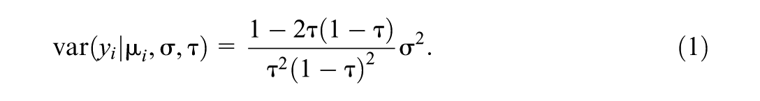
When the AL likelihood is used merely because its maximum coincides with the classical quantile regression estimator, the scale parameter $\mathrm{\sigma }$ appears to be arbitrary. K. Yu and Moyeed (2001) used $\mathrm{\sigma }=1$ without any discussion, and K. Yu and Stander (2007) refer to $\mathrm{\sigma }$ as a “nuisance parameter.” Sriram et al. (2013) proved posterior consistency of the point estimator of $\mathrm{\beta }\left(\mathrm{\tau }\right)$ both when $\mathrm{\sigma }=1$ and when $\mathrm{\sigma }$ is given a prior. Yue and Rue (2011) estimate the scale parameter, arguing that it “makes AL distributions more flexible to capture the unknown error distributions.” The AL error has variance

$$\mathrm{var}(y_i|{\mathrm{\mu }}_i,\mathrm{\sigma },\mathrm{\tau })=\frac{1-2\mathrm{\tau }(1-\mathrm{\tau })}{{\mathrm{\tau }}^2{(1-\mathrm{\tau })}^2}{\mathrm{\sigma }}^2.$$

(1)

We do not know of any papers that set $\mathrm{\sigma }$ to a constant while also considering whether the resulting AL error variance is plausible for the data being analyzed. For example, for their immunoglobulin-G dataset example, K. Yu and Moyeed (2001) set $\mathrm{\sigma }=1$ for both $\mathrm{\tau }=0.50$ and $\mathrm{\tau }=0.95$ , and this corresponds to error variances of 8.0 and 401.1, respectively. Neither variance is plausible because the response variable has a marginal sample variance of 5.2. In fact, the error variance depends so strongly on $\mathrm{\tau }$ that it would never make sense to set $\mathrm{\sigma }$ to the same constant for both the median and extreme quantiles if the analyst is concerned with the plausibility of the AL error variance.

When $\mathrm{\sigma }$ is estimated, the most common prior for $\mathrm{\sigma }$ seems to be an inverse Gamma prior (Kozumi & Kobayashi, 2011; Sriram, 2015; J. Wang, 2012; Yue & Rue, 2011), the conjugate prior under prior independence between $\mathrm{\sigma }$ and $\mathrm{\beta }\left(\mathrm{\tau }\right)$ (Kozumi & Kobayashi, 2011). This prior is used by the R package BayesQR and Stata’s bayes:qreg command, although the latter also allows $\mathrm{\sigma }$ to be set to a constant. Reich et al. (2010) use a uniform prior on $(0,10)$ for $\mathrm{\sigma }$ , and brms uses a half-t distribution with 3 degrees of freedom, which we will denote half-t(3).

2.2. Standard Error Adjustment

While many simulation studies evaluating AL-based Bayesian quantile regression focus exclusively on point estimation, Reich et al. (2010), Sriram (2015), Yang et al. (2016), Lee (2020), and Ji (2022) show that model-based credible intervals have poor coverage.

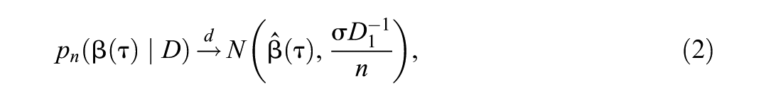
Let ${\mathrm{\beta }}^0\left(\mathrm{\tau }\right)$ be the true parameters of interest and $\hat{\mathrm{\beta }}\left(\mathrm{\tau }\right)$ their ML estimates for a given dataset $D$ . Yang et al. (2016) show that, for flat (improper) priors for the coefficients $\mathrm{\beta }\left(\mathrm{\tau }\right)$ and fixed $\sigma$ , the posterior distribution of $\mathrm{\beta }\left(\mathrm{\tau }\right)$ is asymptotically multivariate normal,

$$p_n(\mathrm{\beta }\left(\mathrm{\tau }\right)\mid D)\stackrel{d}{\to }N(\hat{\mathrm{\beta }}\left(\mathrm{\tau }\right),\frac{\mathrm{\sigma }{D}_1^{-1}}{n}),$$

(2)

where

$$D_1=\underset{n\to \infty }{\lim }\frac{1}{n}\sum _{i=1}^n{f}_{\mathrm{ALD}}(y_i|{\mathrm{\mu }}_i^0,\mathrm{\sigma },\mathrm{\tau })x_i{x}_i^{\prime },$$

with ${\mathrm{\mu }}_i^0=x_i^{\prime }{\mathrm{\beta }}^0\left(\mathrm{\tau }\right)$ . See also Sriram (2015) for the same result when $\mathrm{\sigma }=1$ and $\mathrm{\beta }\left(\mathrm{\tau }\right)$ has an arbitrary proper prior, with Remark 4 generalizing the result to arbitrary fixed $\mathrm{\sigma }$ .

As shown in Equation 2, the asymptotic posterior covariance matrix is proportional to the arbitrary scale parameter $\mathrm{\sigma }$ . Therefore, not surprisingly, it has been demonstrated empirically that credible intervals based on the estimated posterior covariance matrix $\hat{\mathrm{\Sigma }}\left(\mathrm{\sigma }\right)$ , for arbitrarily fixed $\mathrm{\sigma }$ , do not have correct coverage (Ji, 2022; Lee, 2020; Sriram, 2015; Yang et al., 2016).

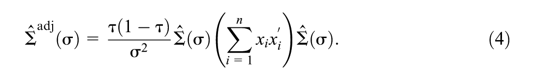
Yang et al. (2016) proposed a simple adjustment to the posterior covariance matrix to improve the coverage of credible intervals. The adjustment is based on Equation 2 and the asymptotic sampling distribution of the ML estimator (Koenker, 2005, p. 74)

$$\sqrt{n}\hat{\mathrm{\beta }}\left(\mathrm{\tau }\right){\to }^{d}N({\mathrm{\beta }}^0,\mathrm{\tau }(1-\mathrm{\tau })D_1^{-1}{D}_0{D}_1^{-1}),$$

(3)

where

$$D_0=\underset{n\to \infty }{\lim }\frac{1}{n}\sum _{i=1}^n{x}_i{x}_i^{\prime }.$$

The adjusted standard errors by Yang et al. (2016) are obtained by substituting $\frac{n}{\mathrm{\sigma }}\hat{\mathrm{\Sigma }}\left(\mathrm{\sigma }\right)$ for $D_1^{-1}$ , based on Equation 2, and estimating $D_0$ by its finite-sample counterpart $n^{-1}\sum _{i=1}^n{x}_i{x}_i^{\prime }$ in the asymptotic “sandwich” covariance matrix $\frac{\mathrm{\tau }(1-\mathrm{\tau })}{n}{D}_1^{-1}{D}_0{D}_1^{-1}$ from Equation 3:

$${\hat{\mathrm{\Sigma }}}^{\mathrm{adj}}\left(\mathrm{\sigma }\right)=\frac{\mathrm{\tau }(1-\mathrm{\tau })}{{\mathrm{\sigma }}^2}\hat{\mathrm{\Sigma }}\left(\mathrm{\sigma }\right)\left(\sum _{i=1}^n{x}_i{x}_i^{\prime }\right)\hat{\mathrm{\Sigma }}\left(\mathrm{\sigma }\right).$$

(4)

Using similar reasoning, Sriram (2015) proposed a two-step approach. In the first step, estimate the posterior means $\tilde{\mathrm{\beta }}\left(\mathrm{\tau }\right)$ and posterior covariance matrix $\hat{\mathrm{\Sigma }}\left(\mathrm{\sigma }\right)$ for $\mathrm{\beta }\left(\mathrm{\tau }\right)$ based on the AL likelihood with fixed $\mathrm{\sigma }$ . In the second step, construct a “sandwich likelihood” that is multivariate normal with means $\tilde{\mathrm{\beta }}\left(\mathrm{\tau }\right)$ and covariance matrix given in Equation 4 and reestimate the posterior means and covariance matrix for $\mathrm{\beta }\left(\mathrm{\tau }\right)$ with the sandwich likelihood replacing the AL likelihood. Sriram (2015) proves that the credible sets from the posterior in Step 2 merge asymptotically with the frequentist confidence sets under mild assumptions.

Yang et al. (2016) argue that ${\hat{\mathrm{\Sigma }}}^{\mathrm{adj}}\left(\mathrm{\sigma }\right)$ is asymptotically invariant to the value of $\mathrm{\sigma }$ and yields asymptotically valid posterior inferences. They demonstrate stability of their intervals for an application with $\mathrm{\tau }=0.5$ and $n=753$ and with $\mathrm{\sigma }$ ranging from 1 to 1,096. However, generally, the posterior distribution may not be well approximated by a multivariate normal distribution with covariance matrix $\frac{\mathrm{\sigma }{D}_1^{-1}}{n}$ , depending on the sample size $n$ , the quantile level $\mathrm{\tau }$ , the value of the scale parameter $\mathrm{\sigma }$ , and the data-generating process. When the approximation does not work, the choice of $\mathrm{\sigma }$ may influence the adjusted covariance matrix.

Yang et al. (2016) recommend setting $\mathrm{\sigma }$ equal to its ML estimate under the AL likelihood for $\mathrm{\tau }=0.5$ , the median. No proof or arguments are provided for this recommendation, and it is not emphasized, presumably due to the assumed approximate invariance of ${\hat{\mathrm{\Sigma }}}^{\mathrm{adj}}\left(\mathrm{\sigma }\right)$ to $\mathrm{\sigma }$ .

For the broader class of approaches that choose a likelihood because its maximum minimizes a loss function, Syring and Martin (2019) propose a hybrid bootstrap-stochastic approximation algorithm for tuning the scale parameter so that the credible intervals have approximately correct frequentist coverage. Such an approach could be used in AL-based Bayesian quantile regression but it would be computationally intensive and is therefore not pursued further here.

In the next section, we introduce IJ standard errors that require little additional computation and, as we demonstrate in Sections 4 and 5, retain approximately correct frequentist properties across a wide range of values of $\mathrm{\sigma }$ and $\mathrm{\tau }$ and for a sample size as low as $n=200$ .

3. IJ Standard Errors

IJ standard errors were originally proposed for frequentist estimators (Jaeckel, 1972) and applied in covariance structure analysis by Jennrich (2008). A Bayesian version, which we will simply denote IJ for brevity, was introduced by Giordano and Broderick (2024), based on their earlier work (Giordano, 2020; Giordano et al., 2018, 2020). Giordano (2020) motivates the IJ variance as an approximation to a resampling variance, such as bootstrap or jackknife. Since it would be computationally infeasible to perform MCMC estimation in a large number of resampled datasets, Giordano et al. (2020) propose using a linear approximation for the posterior means of the parameters in resampled data. Let $w$ be an $n$ -dimensional weight vector, with element $w_i$ equal to the number of times unit $i$ is represented in the resampled data. The part of the posterior distribution that changes in resampled data is the likelihood function, and we can express the log-likelihood for a given weight vector as

$$\sum _{i=1}^n{w}_i{\ell }_i(D|\mathrm{\theta }),$$

where ${\ell }_i(D|\mathrm{\theta })$ is the log-likelihood contribution from unit $i$ for parameter vector $\mathrm{\theta }$ .

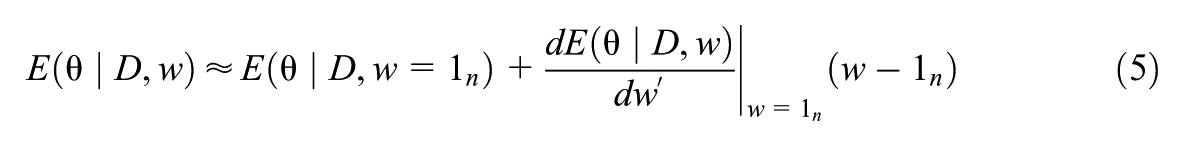
The linear approximation to the posterior expectation for the resampled data is then

$$E(\mathrm{\theta }\mid D,w)\approx E(\mathrm{\theta }\mid D,w=1_n)+{\frac{\mathrm{dE}(\mathrm{\theta }\mid D,w)}{d{w}^{\prime }}|}_{w=1_n}(w-1_n)$$

(5)

$$=E(\mathrm{\theta }\mid D,w=1_n)+{\mathrm{cov}}_{\mathrm{\theta }\mid D}[\mathrm{\theta },\ell (D\mid \mathrm{\theta })](w-1_n),$$

(6)

where all vectors are column vectors, $\mathrm{\theta }$ is $p$ -dimensional, $\ell (D\mid \mathrm{\theta })$ is the $n$ -dimensional vector of log-likelihood contributions from the units, and $1_n$ is an $n$ -dimensional vector with all elements equal to 1. The first term is the posterior expectation for the original dataset. The result that the $p\times n$ matrix of derivatives in Equation 5 is replaced by the posterior covariance matrix of the parameters and log-likelihood contributions in Equation 6 is given in Theorem 1 of Giordano et al. (2018) and derived in section 2 of Efron (2015), as outlined in Supplemental Appendix A. This covariance matrix can be estimated straightforwardly by the corresponding empirical covariance matrix of the MCMC samples.

The influence score for the posterior expectation is then given by

$$I_i:=n{\frac{\mathrm{dE}(\mathrm{\theta }\mid D,w)}{d{w}_i}|}_{w=1_n}=n{\mathrm{cov}}_{\mathrm{\theta }\mid D}[\mathrm{\theta },{\ell }_i(D\mid \mathrm{\theta })],$$

with its estimate from MCMC samples denoted $\widehat{I_i}$ , and the corresponding IJ variance estimator is

$${\hat{V}}^{\mathrm{IJ}}:=\frac{1}{n(n-1)}\sum _{i=1}^n({\hat{I}}_i-\overline{\hat{I}}){({\hat{I}}_i-\overline{\hat{I}})}^{\prime },$$

where $\overline{\hat{I}}$ is the sample mean of the estimated influence score. Both ${\hat{I}}_i$ and $\overline{\hat{I}}$ are $p$ -dimensional column vectors.

3.1. Clustered Data

Cross-sectional clustered data (e.g., patients nested in hospitals, residents nested in street blocks, students nested in classes) and longitudinal data violate the independence assumption of the AL likelihood and of IJ standard errors.

There have been several approaches to explicitly modeling between-cluster heterogeneity and/or within-cluster dependence in quantile regression. In a non-Bayesian setting, Koenker and Hallock (2004) propose a model for longitudinal data that includes subject-specific fixed effects ${\mathrm{\alpha }}_i\left(\mathrm{\tau }\right)$ in the linear conditional quantile model. They also include an ${\ell }_1$ (Lasso) penalty for these fixed effects to shrink them toward a common intercept. Lamarche and Parker (2023) propose a bootstrapping procedure for the standard errors of this model. Also in a non-Bayesian setting, Geraci and Bottai (2007, 2014) define linear quantile mixed models that resemble linear mixed models by including normally distributed cluster-specific random effects in the linear conditional quantile function, with an AL distribution for the (level-1) errors. Bayesian quantile regression models with cluster-specific random effects have also been proposed, both with an AL likelihood (Luo et al., 2012; J. Wang, 2012; Y. Yu, 2015) and with more flexible densities for the level-1 errors, such as an infinite mixture of normal densities (Reich et al., 2010).

In quantile regression models with cluster-specific fixed or random effects, the regression coefficients represent the relationship between cluster-specific quantiles and the covariates and do not have any meaningful marginal (over the clusters) interpretation (see, e.g., Reich et al., 2010). Here, we focus on models for the marginal quantiles. Such a marginal approach was also adopted, for instance, by Lipsitz et al. (1997) in Biostatistics, and Parente and Silva (2016) as well as Hagemann (2017) in Econometrics. For example, Hagemann (2017) ignores the clustering for point estimation and develops a bootstrap procedure for obtaining cluster-robust standard errors. Here, we propose adopting such an approach but with a clustered-data version of the IJ standard errors instead of bootstrapping.

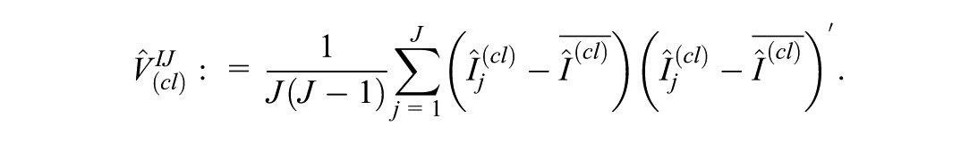
Specifically, letting $J$ be the number of clusters and $n$ the total sample size, we define the influence score for cluster $j$ as

$$I_j^{\left(\mathrm{cl}\right)}:=J\sum _{\begin{array}{c}i\hfill \\ \multicolumn{1}{c}{\mathrm{in}\mathrm{cluster}j}\end{array}}\frac{I_i}{n},$$

denote its estimate from MCMC samples as ${\hat{I}}_j^{\left(\mathrm{cl}\right)}$ , and estimate the variance as

$${\hat{V}}_{\left(\mathrm{cl}\right)}^{\mathrm{IJ}}:=\frac{1}{J(J-1)}\sum _{j=1}^J({\hat{I}}_j^{\left(\mathrm{cl}\right)}-\overline{{\hat{I}}^{\left(\mathrm{cl}\right)}}){({\hat{I}}_j^{\left(\mathrm{cl}\right)}-\overline{{\hat{I}}^{\left(\mathrm{cl}\right)}})}^{\prime }.$$

This approach can be justified from a resampling perspective where entire clusters are resampled. Equivalently, we can define

$$I_j^{\left(\mathrm{cl}\right)}:=J{\mathrm{cov}}_{\mathrm{\theta }\mid D}[\mathrm{\theta },{\ell }_j^{\left(\mathrm{cl}\right)}(D\mid \mathrm{\theta })],$$

where

$${\ell }_j^{\left(\mathrm{cl}\right)}:=\sum _{\begin{array}{c}i\hfill \\ \multicolumn{1}{c}{\mathrm{in}\mathrm{cluster}j}\end{array}}{\ell }_i(D\mid \mathrm{\theta }).$$

4. Evaluation of Standard Errors for Independent Data

4.1. Methods

We consider two data-generating models: (1) location-shifted normal, and (2) location-shifted and scaled normal.

• Model 1: Location-shifted normal model—The data-generating model is

$$y_i=\mathrm{\alpha }+\mathrm{\beta }{x}_i+{ϵ}_i,{ϵ}_i~N(0,1).$$

The corresponding function for the $\mathrm{\tau }\mathrm{t}\mathrm{h}$ conditional quantile is

$$Q_{\mathrm{\tau }}(y_i\mid x_i)=[\mathrm{\alpha }+{\mathrm{\Phi }}^{-1}\left(\mathrm{\tau }\right)]+\mathrm{\beta }{x}_i,$$

so that the slope of $x_i$ is constant across quantile levels and the location (or intercept) at quantile level $\mathrm{\tau }\ne 0.5$ is shifted by ${\mathrm{\Phi }}^{-1}\left(\mathrm{\tau }\right)$ relative to the intercept at the median, where $\mathrm{\Phi }$ is the standard normal CDF.

• Model 2: Location-shifted and scaled normal model—The model is

$$y_i=\mathrm{\alpha }+\mathrm{\beta }{x}_i+(1+\mathrm{\gamma }{x}_i){ϵ}_i,{ϵ}_i~N(0,1),$$

with conditional standard deviation $\mathrm{sd}(y_i|x_i)=|1+\mathrm{\gamma }{x}_i$ and conditional quantile function

$$Q_{\mathrm{\tau }}(y_i\mid x_i)=[\mathrm{\alpha }+{\mathrm{\Phi }}^{-1}\left(\mathrm{\tau }\right)]+[\mathrm{\beta }+\mathrm{\gamma }{\mathrm{\Phi }}^{-1}\left(\mathrm{\tau }\right)]x_i.$$

Now the slopes of $x_i$ at different quantile levels are no longer constant but are shifted by $\mathrm{\gamma }{\mathrm{\Phi }}^{-1}\left(\mathrm{\tau }\right)$ relative to the slope at the median.

For the models above, we consider two choices of sample size ( $n=200$ and $n=1,000$ ), simulate $x_i$ from a standard Gaussian distribution, and fix $\mathrm{\alpha }=\mathrm{\beta }=2$ for both models and $\mathrm{\gamma }=0.3$ for Model 2. We compare various kinds of approximate standard errors and corresponding credible intervals (based on a normal approximation) for five different quantiles, $\mathrm{\tau }\in \{0.1,0.3,0.5,0.7,0.9\}$ .

First, we investigate sensitivity to the scale parameter of the following Bayesian methods:

• ALD: Unadjusted model-based posterior standard deviations.

• IJf: IJ standard errors with fixed $\mathrm{\sigma }$ .

• Yang: Adjusted standard errors proposed by Yang et al. (2016).

Point estimation for these methods is performed using Stan. We set $\mathrm{\sigma }$ to $\{0.1,0.2,0.5,1,2,5,10\}$ . While $\mathrm{\sigma }=1$ is a likely default choice, the magnitude of $\mathrm{\sigma }$ should be assessed in relation to the standard deviation of the response variable because the AL variance is proportional to ${\mathrm{\sigma }}^2$ for a given value of $\mathrm{\tau }$ , as shown in Equation 1. For example, the standard deviation of the response variable is 5.6 times as great for Model 2 here as for the application discussed in Section 6.1 (the standard deviations are 2.25 and 0.40, respectively), making $\mathrm{\sigma }=5.6$ here comparable to the analysis we present in Section 6.1 with $\mathrm{\sigma }=1$ .

Second, we compare IJf, with $\mathrm{\sigma }=1$ , with the following methods that do not rely on setting the scale parameter to an arbitrary constant:

• boot: Frequentist point estimates and bootstrap standard errors (quantreg, R package version 5.95, by Koenker, 2021, with the options se = boot and bsmethod = “xy”).

• sandwich: Frequentist point estimates and standard errors based on the sandwich estimator (quantreg, R package version 5.95, by Koenker (2021), with option se = nid).

• IJ: Bayesian point estimates (posterior means) and IJ standard errors with estimated $\mathrm{\sigma }$ (brms with AL likelihood and half-t(3) prior for $\mathrm{\sigma }$ and our IJSE package).

• AdjBQR: Posterior means and adjusted standard errors proposed by Yang et al. (2016) with $\mathrm{\sigma }$ fixed at MLE for $\mathrm{\tau }=0.5$ (AdjBQR, R package version 1.0, by H. J. Wang, 2016).

• brms: Posterior means and model-based posterior standard deviations when $\mathrm{\sigma }$ has a half-t(3) distribution (brms, R package version 2.20.1, by Bürkner, 2017).

• BayesQR: Posterior means and model-based posterior standard deviations when $\mathrm{\sigma }$ has an inverse Gamma(.01, .01) prior with scale parameter and shape parameter both equal to 0.01 (BayesQR, R package version 2.4, by Benoit & Van den Poel, 2017).

In both simulation studies, all methods are applied to each of 100 replications. We assess how well the different versions of standard errors approximate the sampling standard deviations of the point estimates of the intercept and slope parameters by reporting the relative error defined as

$$R_e=\sqrt{\frac{\overline{s{e}^2}}{\mathrm{var}\left(\hat{\mathrm{\beta }}\right)}}-1,$$

where $\overline{s{e}^2}$ is the average squared standard error estimate across replications and $\mathrm{var}\left(\hat{\mathrm{\beta }}\right)$ is the variance of the point estimates across replications. The Monte Carlo error (MCe) of this relative error is approximately (White, 2010)

$$\mathrm{MCe}=(R_e+1)\sqrt{\frac{\mathrm{var}\left(s{e}^2\right)}{\mathrm{var}{\left(\hat{\mathrm{\beta }}\right)}^2}+\frac{1}{(2m-1)}},$$

where $m=100$ is the number of replications. We also present approximate 95% confidence intervals for the relative error based on the MCe.

Finally, we report empirical coverage of 90% credible intervals (using a normality-based approximation centered at the posterior mean) along with exact binomial 95% confidence intervals for the coverage.

4.2. Results

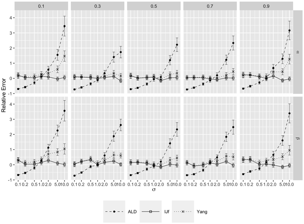
Figure 1 shows the relative error for ALD (solid line), IJf (dotted line), and Yang (dashed line) as a function of the scale parameter $\mathrm{\sigma }$ for the intercept $\mathrm{\alpha }$ (row 1) and slope $\mathrm{\beta }$ (row 2) and different quantile levels $\mathrm{\tau }$ (columns) for Model 2 with $n=200$ . Analogous figures for Model 1 and $n=1,000$ are given in Supplemental Appendix B. It is clear that the model-based posterior standard deviations (denoted ALD) can either over- or under estimate the uncertainty depending on the value of the scale parameter, with standard errors being as much as 300% too large for the range of scale parameters considered. As $\mathrm{\sigma }$ increases, the data appear less informative, leading to larger model-based posterior standard deviations. While Yang performs better than ALD, it produces unsatisfactory results (such as being over 50% too large) for some of the values of $\mathrm{\sigma }$ considered, especially for quantile levels 0.1 and 0.9. In contrast, the relative error of IJf is close to zero across the range of scale parameters considered.

Figure 1.

Relative error with approximate 95% confidence intervals for different types of standard errors as a function of the scale parameter $\mathrm{\sigma }$ for different quantiles (t) for Model 2 with n = 200.

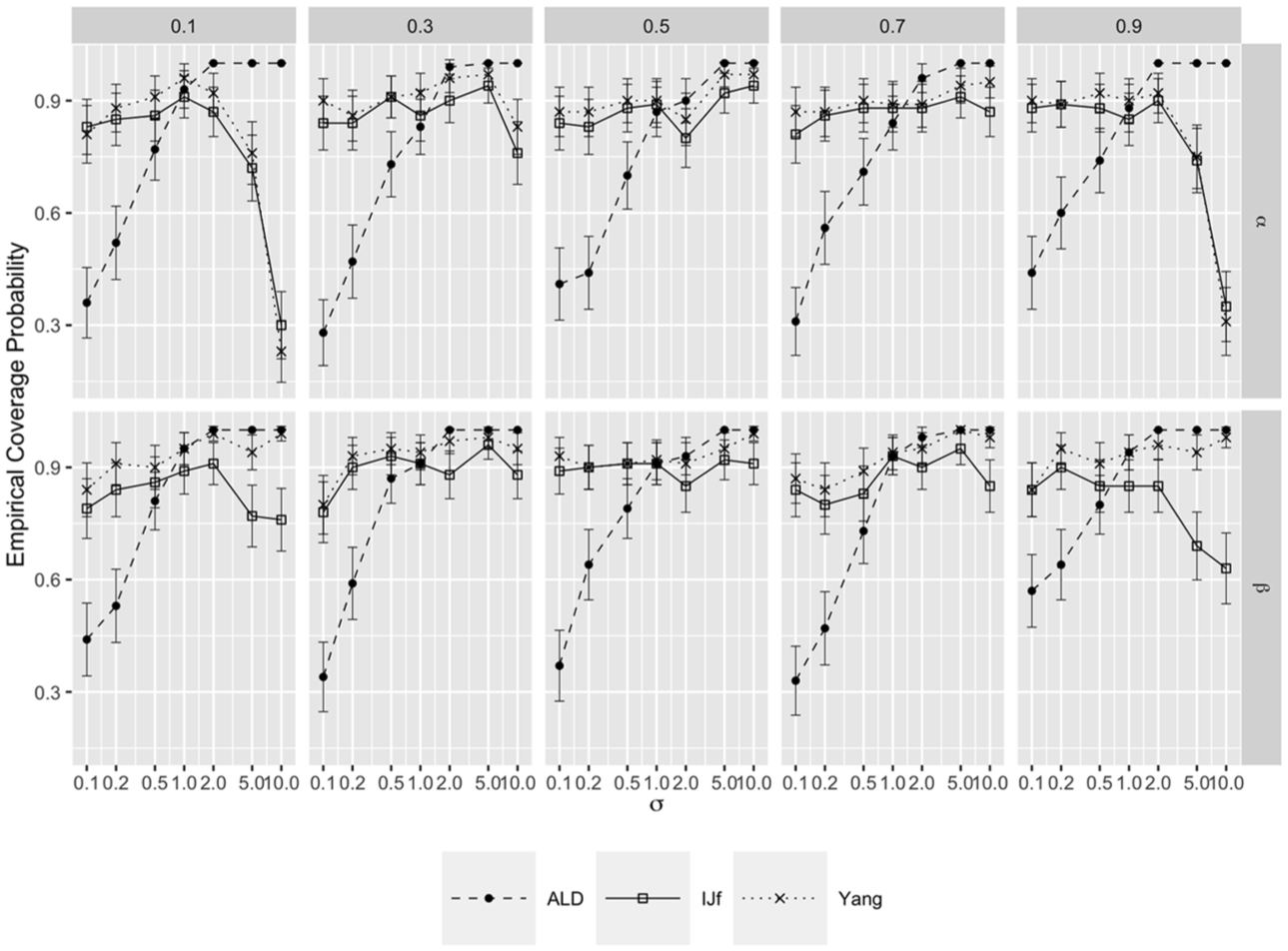
Figure 2 shows the empirical coverage of 90% credible intervals with exact binomial 95% confidence intervals for Model 2 with $n=200$ , in the same format as Figure 1. Analogous graphs for Model 1 and $n=1,000$ are given in Supplemental Appendix B.

Figure 2.

Empirical coverage of 90% credible intervals for different types of standard errors as a function of the scale parameter $\mathrm{\sigma }$ for different quantiles ( $\tau$ ) for Model 2 with n = 200.

As expected, ALD performs poorly for both $\mathrm{\alpha }$ and $\mathrm{\beta }$ , at all quantile levels, for most values of $\mathrm{\sigma }$ , with decreasing undercoverage as $\sigma$ increases to about 1 and then increasing overcoverage as $\mathrm{\sigma }$ continues to increase. For non-extreme quantiles (i.e., $\mathrm{\tau }=0.3,0.5,\mathrm{or}0.7$ ), coverage of the proposed IJf method is similar to that of the frequentist sandwich and bootstrap methods, all at around the nominal 0.9 level, across different choices of the scale parameter $\mathrm{\sigma }$ , sample size, and data-generating model.

However, for the two extreme quantiles with large scale parameter (i.e., $\mathrm{\tau }=0.1\mathrm{or}0.9$ and $\mathrm{\sigma }=5\mathrm{or}10$ ), coverage of the IJf intervals for both the intercept and the slope is too low, especially for the intercept. A reason for this undercoverage is that the Bayesian point estimator for the intercept is severely biased for extreme quantiles with large scale parameters, as also observed in previous simulation studies (Lee, 2020, pp. 48–49). For example, when $\mathrm{\tau }=0.9$ , $\mathrm{\sigma }=10$ , the bias for $\mathrm{\beta }$ is estimated as 0.2 for Model 2 with $n=200$ . In this simulation condition, IJf has under-coverage because its standard error reflects the sampling standard deviation, as shown in Figure 1, whereas Yang has over-coverage (0.99) because the adjusted standard error is too large. Specifically, the average Yang standard error is 0.2 compared with 0.09 for IJf. Briefly, the reason for the bias seems to be that the posterior distribution of the intercept becomes increasingly skewed as $\mathrm{\tau }$ becomes more extreme (further from 0.5) and as $\mathrm{\sigma }$ increases, so that the posterior mean differs increasingly from the posterior mode. However, the AL likelihood is chosen because its mode corresponds to the classical estimator. See also Section 6.1 for an illustration of this phenomenon.

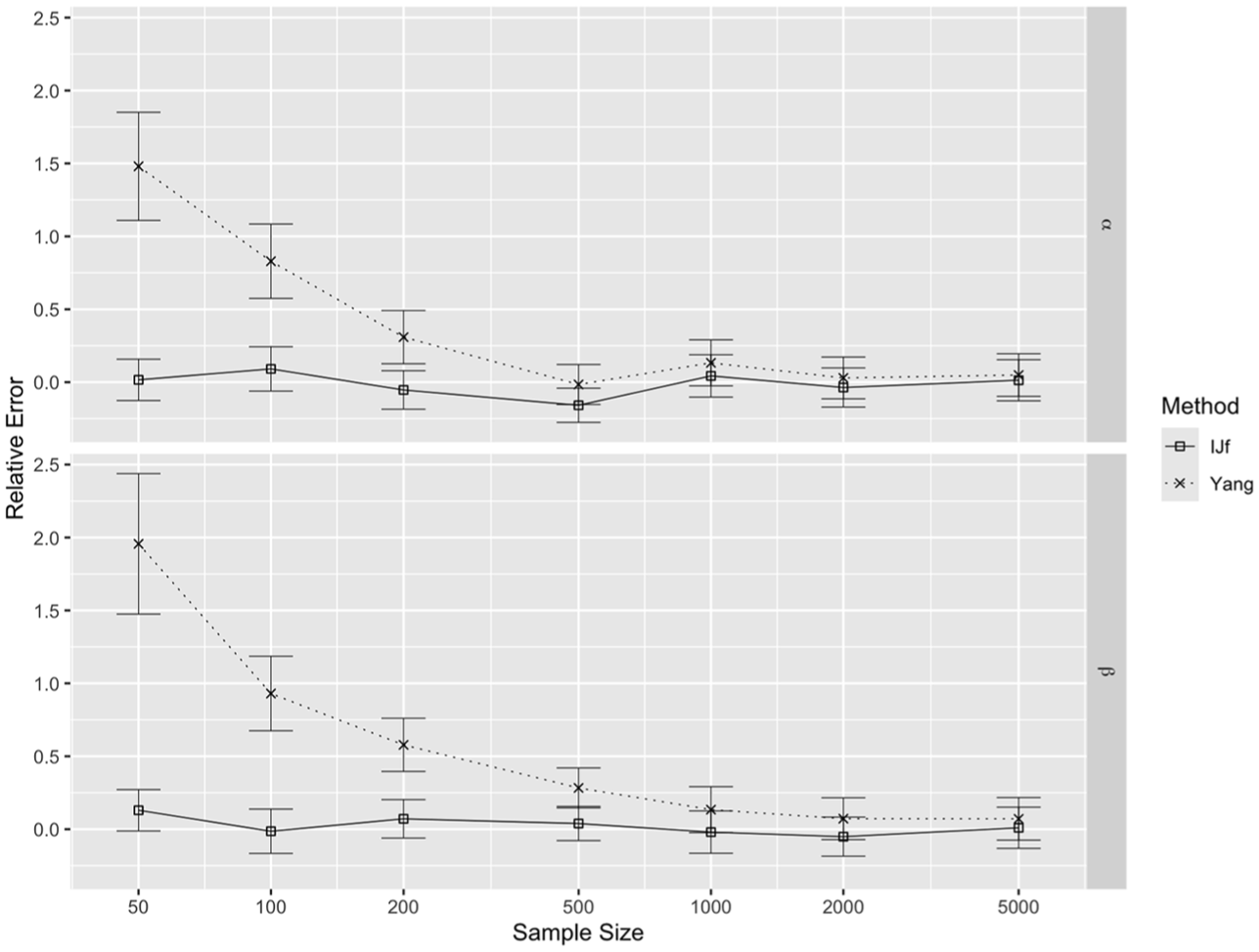
As Yang relies on asymptotic results, we further investigated its performance, compared with IJf, for $\mathrm{\sigma }=10$ and $\mathrm{\tau }=0.7$ as the sample size increases from 50 to 5,000. Figure 3 shows that the relative error for Yang decreases as the sample size increases, as expected. Remarkably, IJf standard errors are approximately correct for sample sizes as low as 50. However, the estimator may be biased at small sample sizes, and this would diminish the utility of obtaining a correct standard error. For example, at $n=50$ , the bias for $\mathrm{\beta }$ is estimated as .05, with sampling standard deviation 0.17, and at $n=200$ , the bias is estimated as 0.03, with sampling standard deviation 0.08.

Figure 3.

Relative error of IJf and Yang with approximate 95% confidence intervals as a function of sample size for $\tau =0.7$ , $\sigma =10$ , and Model 2.

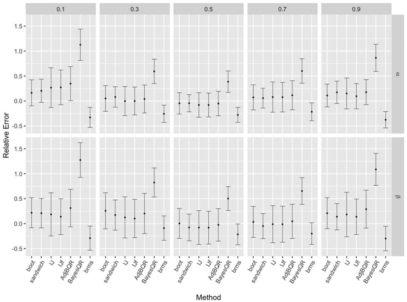
Figure 4 shows the relative error for IJf with $\mathrm{\sigma }=1$ and for the methods that do not rely on fixing the scale parameter for Model 2 with $n=200$ . The results for Model 1 and $n=1,000$ are given in Supplemental Appendix B. IJ, IJf, and AdjBQR (the adjusted standard errors) perform well, with relative errors similar to the frequentist methods (boot and sandwich), whereas the unadjusted Bayesian estimates that treat $\mathrm{\sigma }$ as a free parameter (BayesQR and brms) perform worse. BayesQR consistently performs rather poorly compared to all other methods, and hence we do not include it in the remainder of the paper. brms, which is commonly used in practice, underestimates the standard errors for $\mathrm{\alpha }$ across quantile levels and for $\mathrm{\beta }$ at the extreme quantile levels ( $\mathrm{\tau }=0.1$ and $\mathrm{\tau }=0.9$ ).

Figure 4.

Relative error with approximate 95% confidence intervals for different methods with $\mathrm{n}=200$ and Model 2.

5. Evaluation of Standard Errors for Clustered Data

To make our simulation results comparable to the results presented by Hagemann (2017) for cluster-robust inference for quantile regression, we follow his simulation setup. The data-generating model is

$$y_{\mathrm{ij}}=\frac{1}{10}{u}_{\mathrm{ij}}+x_{\mathrm{ij}}+x_{\mathrm{ij}}^2{u}_{\mathrm{ij}},$$

where $x_{\mathrm{ij}}$ is the sum of $\sqrt{\mathrm{\rho }}{z}_j$ and $\sqrt{1-\mathrm{\rho }}{ϵ}_{\mathrm{ij}}$ with $\mathrm{\rho }\in [0,1)$ , $z_j~N(0,1)$ and, independently, ${ϵ}_{\mathrm{ij}}~N(0,1)$ , so that $x_{\mathrm{ij}}$ has an intraclass correlation equal to $\mathrm{\rho }$ and a variance of 1. Finally, $u_{\mathrm{ij}}~N(0,\frac{1}{3})$ . This outcome model implies that the conditional quantile functions are

$$Q_{\tau }(y_{\mathrm{ij}}\mid x_{\mathrm{ij}})=\mathrm{\alpha }\left(\mathrm{\tau }\right)+{\mathrm{\beta }}_1\left(\mathrm{\tau }\right)x_{\mathrm{ij}}+{\mathrm{\beta }}_2\left(\mathrm{\tau }\right)x_{\mathrm{ij}}^2,$$

with $\mathrm{\alpha }\left(\mathrm{\tau }\right)=\frac{{\mathrm{\Phi }}^{-1}\left(\mathrm{\tau }\right)}{\sqrt{300}}$ , ${\mathrm{\beta }}_1\left(\mathrm{\tau }\right)=1$ , and ${\mathrm{\beta }}_2\left(\mathrm{\tau }\right)=\frac{{\mathrm{\Phi }}^{-1}\left(\mathrm{\tau }\right)}{\sqrt{3}}$ .

We consider two cluster sizes, $I\in \{10,30\}$ , three choices of number of clusters, $J\in \{10,50,100\}$ , two choices of intraclass correlation, $\mathrm{ICC}\in \{0.3,0.8\}$ , and five quantile levels, $\mathrm{\tau }\in \{0.1,0.3,0.5,0.7,0.9\}$ . We compare IJf (with $\mathrm{\sigma }=0.1$ ), with IJ and the current state-of-the-art clustered gradient bootstrap (denoted boot) defined in the study by Hagemann (2017) for frequentist quantile regression.

The relative error of the standard errors and empirical coverage of the corresponding 90% intervals are estimated, and both are reported with 95% confidence intervals.

5.1. Results

Results for only $J=10$ clusters are not shown here because none of the methods consistently performed well in this case. As shown in Supplemental Appendix C, with $J=10$ , the relative error for bootstrap standard errors was large (sometimes off the scale of the figures) for the extreme quantiles ( $\mathrm{\tau }=0.1$ and $\mathrm{\tau }=0.9$ ), because the bootstrap standard errors were extremely large for some simulated datasets under these conditions. While the relative error for IJ and IJf is close to zero, we observed undercoverage of IJ and IJf intervals when $J=10$ , particularly for ${\mathrm{\beta }}_2$ and for the extreme quantiles, possibly due to poor point estimation with the smaller total sample sizes ( $n=100$ or $300$ for $J=10$ ). In contrast, bootstrap intervals sometimes show overcoverage for extreme quantiles. We therefore recommend against using any of these methods for the extreme quantiles when $J=10$ .

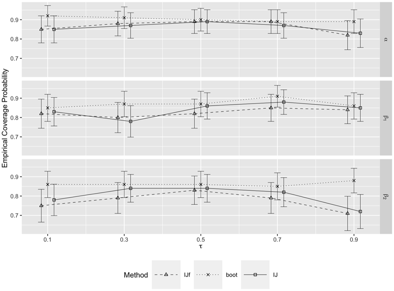
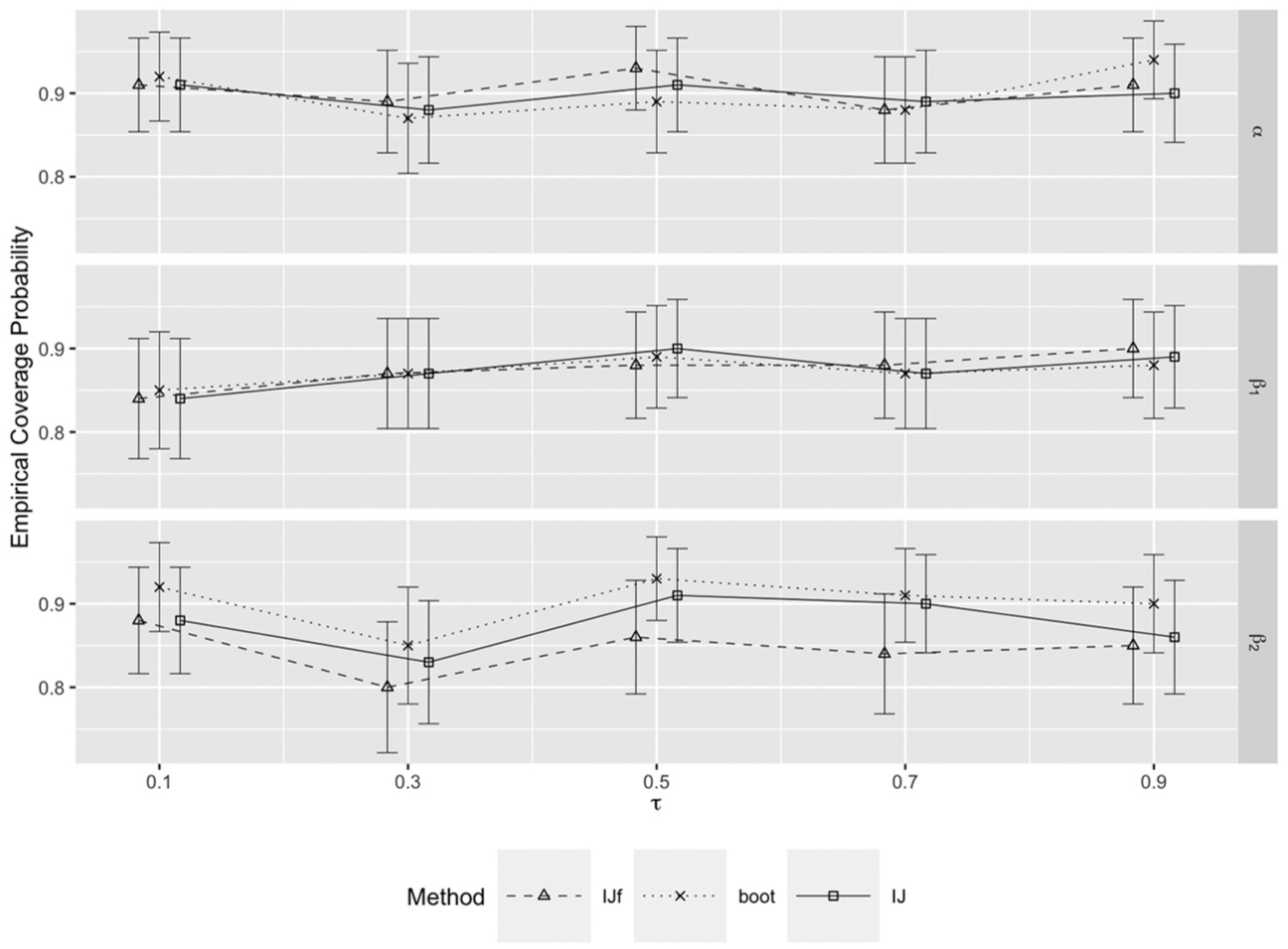
Here, we present the empirical coverage for the smallest sample size considered with $J>10$ , that is, $I=10$ , $J=50$ in Figure 5, and for the largest sample size considered, that is, $I=30$ , $J=100$ in Figure 6, both for $\mathrm{\rho }=0.8$ . In both conditions, coverage tends to be closer to the nominal level for IJ than for IJf, and the confidence intervals mostly span 0.9, except for ${\mathrm{\beta }}_2$ , at the extreme quantiles, with the smaller total sample size. The results for the other conditions are presented in Supplemental Appendix C.

Figure 5.

Empirical coverage probability as a function of $\tau$ for $I=10$ , $J=50$ , $\rho =0.8$ .

Figure 6.

Empirical coverage probability as a function of $\tau$ for $I=30$ , $J=100$ , $\rho =0.8$ .

6. Applications

For the applications, we will estimate the scale parameter (use IJ rather than IJf) as this approach does not rely on finding a suitable value of the scale parameter and tends to perform better than IJf in the simulations. We will compare IJ-based intervals with intervals based on alternative standard errors for two real datasets.

6.1. Income and Food Expenditure

Here, we follow Koenker and Bassett (1982) in analyzing data from Engel (1857) on household income and food expenditure. This dataset is also used in the Stata manual (StataCorp, 2023a) for demonstrating their AL-based Bayesian quantile regression. As it is in the public domain, this dataset serves as a useful benchmark for comparing standard error estimates.

Engel used the data to show that “The poorer a family, the greater the part of total expenditures must be spent on food,” later referred to as Engel’s law (Perthel, 1975). The data provided as Engel1867.dta with the Stata software consists of annual household income and annual food expenditure, in thousands of Belgian Franks, for 235 European working-class households in the 19th century.

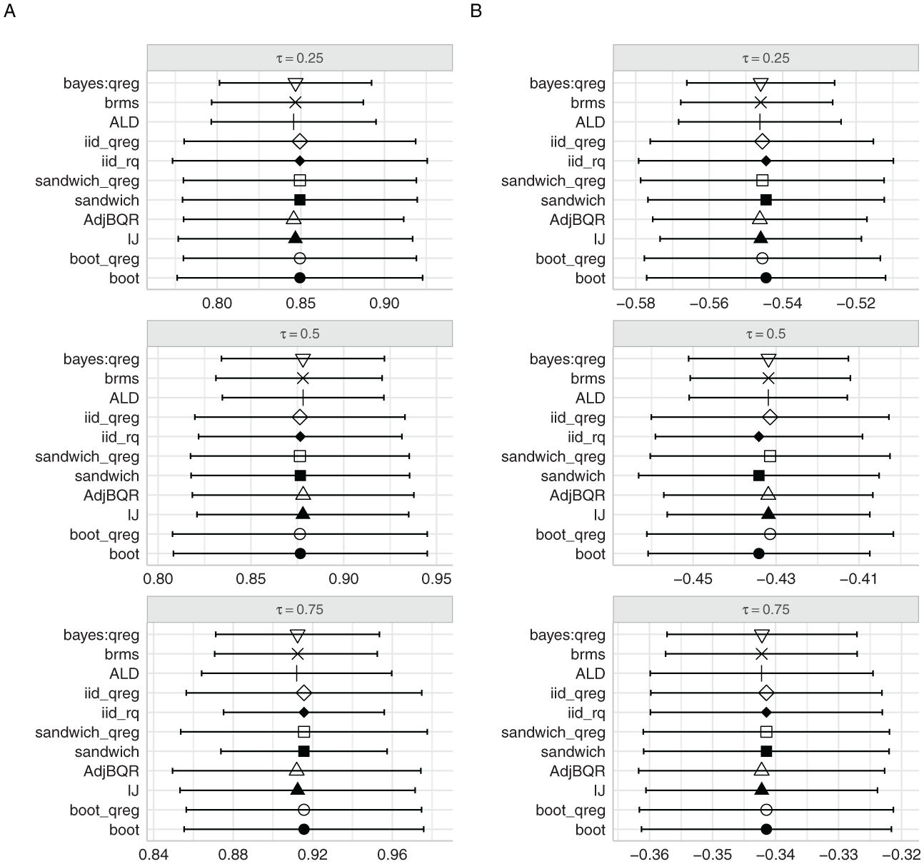
Performing quantile regression with log-expenditure as response variable and log-income as explanatory variable, Koenker and Bassett (1982) report slope estimates (that they refer to as Engel elasticities) of 0.85, 0.88, and 0.92 for $\mathrm{\tau }=0.25,\mathrm{\tau }=0.50$ , and $\mathrm{\tau }=0.75$ , respectively. We fitted the quantile regression models to Engel’s data using various methods, and Figure 7 shows the point estimates with 95% credible intervals/confidence intervals for the slope (panel A) and intercept (panel B) for $\mathrm{\tau }=0.25$ , $\mathrm{\tau }=0.50$ , and $\mathrm{\tau }=0.75$ . The methods used were the same as those used in the simulations (ALD, here with $\mathrm{\sigma }$ set to its MLE at the median, IJ, boot, sandwich, AdjBQR, brms) plus the following:

• bayes:qreg: AL-based Bayesian quantile regression using the bayes:qreg command in Stata (StataCorp, 2023a). This method uses an inverse Gamma(.01, .01) prior for $\mathrm{\sigma }$ .

• iid_qreg: Frequentist quantile regression using the Stata qreg command with the default method for computing standard errors, assuming independent and identically distributed (i.i.d.) units.

• iid_rq: Frequentist quantile regression using the rq() function in the quantreg R package, with the option se = iid. The asymptotic covariance matrix for i.i.d. units is computed as described by Koenker and Bassett (1978).

• sandwich_qreg: Frequentist quantile regression using the Stata qreg command with the vce(robust) option to compute the sandwich estimator for non-i.i.d. units by Hendricks and Koenker (1992).

• boot_qreg: Frequentist bootstrapped quantile regression using the bsqreg command in Stata. This method estimates the variance–covariance matrix by randomly resampling the data (De Angelis et al., 1993).

The point estimates and standard error estimates for bayesQR (Benoit & Van den Poel, 2017) were so divergent from the other methods that we decided not to include the bayesQR intervals in Figure 7. Readers interested in these intervals can refer to Supplemental Appendix D.

Figure 7.

Comparison of slope and intercept estimates for log income using various quantile regression methods with approximate 95% credible intervals/confidence intervals. Note that we took the natural logarithm of expenditure and income, both measured in thousands of Franks per year (as in Engel1867.dta). Using log base 10 and units of Franks per year (as in the Engel vignette of the quantreg package) affects the intercept estimates but not the slope estimates. (A) Estimates of slope for log income. (B) Estimates of intercept.

The first notable observation in Figure 7 is that the point estimates for both the slope and intercept are generally similar across methods, whereas the standard error estimates vary significantly. Most importantly, the intervals produced by the brms package in R and the bayes:qreg command in Stata, both of which are publicly available and likely to be chosen by applied researchers, are considerably narrower than most other intervals, a result consistent with the finding in Figure 4 that brms tends to underestimate the standard error. The ALD method shows similar levels of underestimation of standard errors to brms and bayes:qreg.

Second, among the AL-based Bayesian quantile regression options, the two methods that apply some form of standard error correction, that is, AdjBQR and IJ, generally produce standard errors comparable in magnitude to sandwich_qreg, Stata’s sandwich estimator. The bootstrap standard errors tend to be larger, except at $\mathrm{\tau }=0.75$ . The sandwich and iid_rq methods from quantreg underestimate the standard errors for the slope to a degree similar to brms when $\mathrm{\tau }=0.75$ . This underestimation seems to be related to the local estimate of the sparsity in the rq() function of the quantreg package and suggests caution when using quantreg for extreme quantiles.

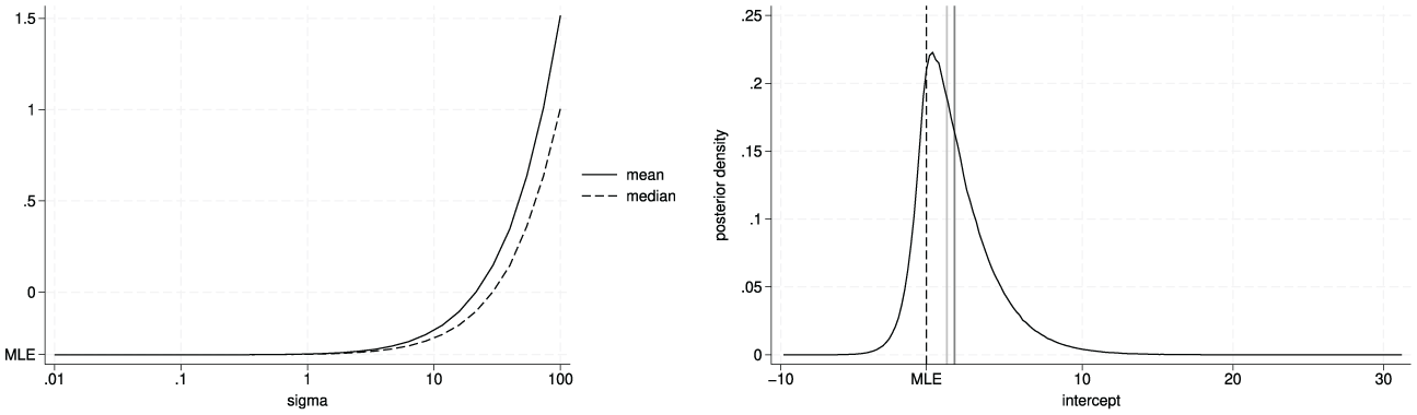
We can also use this dataset to demonstrate that, for an AL likelihood with fixed $\mathrm{\sigma }$ and for $\mathrm{\tau }=0.75$ , the posterior density for the intercept becomes increasingly right-skewed as $\mathrm{\sigma }$ increases. The left panel of Figure 8 shows that the difference between the posterior mean and the median of the intercept increases as $\mathrm{\sigma }$ increases, and that both point estimates increasingly differ from the MLE or posterior mode. The right panel shows the kernel density estimate of the posterior density for $\mathrm{\sigma }=100$ , for which the considerable right-skew of the posterior leads to the posterior mean being larger than the posterior median, which in turn is larger than the posterior mode and MLE (Note that we chose $\mathrm{\sigma }$ as large as $100$ to make the asymmetry obvious).

Figure 8.

Comparison of posterior mean, median, and MLE for $\sigma$ ranging from .01 to 100 (left panel) and for $\sigma =100$ , with kernel density estimate of posterior density (right panel) for the Engel data with $\tau =0.75$ .

6.2. Project STAR

In this section, we analyze data from the Tennessee Student/Teacher Achievement Ratio (STAR) experiment to compare our IJ standard errors for clustered data with estimates presented by Hagemann (2017), who utilized a bootstrap method to obtain cluster-robust standard errors.

In the 1985 to 1986 school year, Project STAR randomly assigned incoming kindergarten students in 79 Tennessee schools to one of three class types: small classes (13–17 students), regular-size classes (22–25 students), and regular-size classes with a full-time teacher’s aide. Teachers were also randomly assigned to these class types. The study included 6,325 students across 325 classrooms, with 5,727 students having complete data for analysis. Hagemann (2017) aimed to estimate the effect of classroom type on student achievement, with standard errors clustered at the classroom level to account for any unobserved between-classroom heterogeneity due to peer effects and unobserved teacher characteristics.

To replicate Hagemann’s (2017) results, we fit a quantile regression model to math and reading test scores from the end of the 1985 to 1986 school year. In this model, the main explanatory variables of interest are the two treatment dummies: small, an indicator for the student being assigned to a small class, and regaide, an indicator for the student being assigned to a regular-sized class with an aide. Additionally, we control for a set of pre-treatment covariates specified in Hagemann (2017), along with school fixed effects.

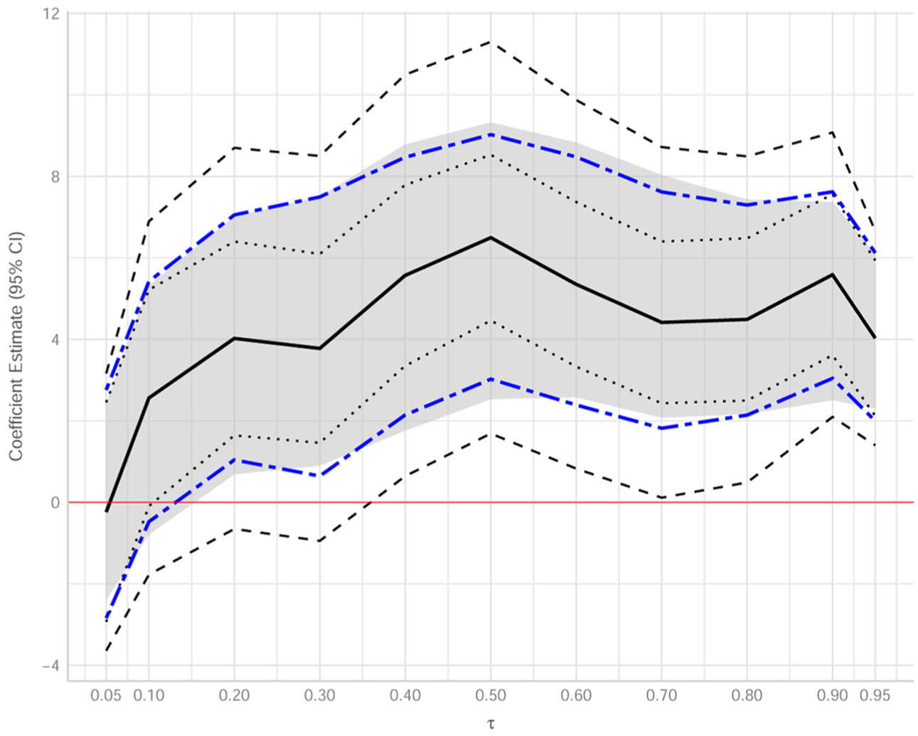
Figure 9 replicates Figure 3 in the study by Hagemann (2017) and additionally presents our IJ standard error results. The solid black line represents the quantile regression coefficient estimates for the treatment dummy small across eleven different quantile levels $\mathrm{\tau }$ , presented as ticks on the x-axis. The dotted lines show the 95% pointwise confidence intervals that do not account for clustering in classrooms. These intervals were obtained by specifying the se = “ker” option for the rq() function in the quantreg package, which uses a kernel estimate of the sandwich as proposed by Powell (1991). The gray band shows the 95% pointwise cluster-robust wild gradient bootstrap confidence intervals proposed by Hagemann (2017), computed by the boot.rq() function in the quantreg package with the cluster option. We used 999 bootstrap simulations to calculate these intervals.

Figure 9.

Quantile regression coefficient estimates and 95% confidence intervals for the coefficient of the treatment dummy small as a function of quantile level $\tau$ .

The two-dashed blue lines in Figure 9 represent 95% pointwise confidence intervals based on our IJ standard errors for clustered data. Here, the brms package was used for point estimation, with an AL likelihood and a half-t(3) prior for $\mathrm{\sigma }$ , and our IJSE package was used to compute IJ standard errors for clustered data as described in Section 3.1. These IJ confidence intervals closely match those based on the cluster-robust bootstrap (The outermost black dashed lines, included to replicate Figure 3 in the study by Hagemann (2017), represent a 95% bootstrap confidence band for the entire quantile regression coefficient function).

7. Concluding Remarks

We have argued and shown empirically that model-based posterior standard deviations are not valid when the scale parameter $\mathrm{\sigma }$ is set to an arbitrary constant, a fact that is not widely known even though it has previously been shown by Sriram (2015), Yang et al. (2016), and others. Tuning $\mathrm{\sigma }$ to achieve good coverage (Syring & Martin, 2019) is one option, and using the expression for the asymptotic covariance matrix to adjust the standard errors (Sriram, 2015; Yang et al., 2016) is another option. However, when the sample size is not very large and a quantile other than the median is of interest, the adjustment by Yang et al. (2016) can perform poorly unless $\mathrm{\sigma }$ is set to a “good” value, one option being its MLE at the median.

Estimating $\mathrm{\sigma }$ along with the model parameters instead of setting it to an arbitrary constant produces better-performing model-based posterior standard deviations, but they were substantially too low across most of our simulation conditions and worse than the adjusted standard errors by Yang et al. (2016) with $\mathrm{\sigma }$ set to its MLE at the median.

We propose using Bayesian IJ standard errors (Giordano & Broderick, 2024) because they have low relative errors regardless of the value to which $\mathrm{\sigma }$ is set. Coverage is also good except at extreme quantiles when $\mathrm{\sigma }$ is such that the point estimates are biased. We have seen little discussion in the literature of bias due to a poor choice of $\mathrm{\sigma }$ . We showed that the bias tends to increase with $\mathrm{\sigma }$ , as the posterior distributions of the regression parameters become increasingly skewed, particularly for the intercept parameter.

If $\mathrm{\sigma }$ is set to a constant, we therefore recommend comparing the posterior mean and median of the intercept or using other ways of assessing the skewness of the posterior. When skewness is severe, estimation should be repeated with a smaller value of $\mathrm{\sigma }$ . Alternatively, $\mathrm{\sigma }$ can be estimated along with the model parameters, and our empirical results suggest that this approach works quite well.

Besides its good performance for quantile regression compared with alternative methods, the IJ approach has several other advantages. One advantage is that IJ standard errors for any function $f\left(\mathrm{\beta }\left(\mathrm{\tau }\right)\right)$ of the model parameters can be obtained by estimating the posterior covariance matrix between $f\left(\mathrm{\beta }\left(\mathrm{\tau }\right)\right)$ and the log-likelihood contributions (Giordano & Broderick, 2024). Examples of such nonlinear functions are indirect and total effects in mediation analysis (Falk et al., 2024; Yuan & MacKinnon, 2009), standardized regression coefficients (Dudgeon, 2017), and reliability coefficients in psychometrics (Raykov, 2002). Another advantage, demonstrated in this paper, is that the IJ approach can be used for clustered data, with similar performance as frequentist estimation with bootstrap standard errors. Finally, IJ standard errors are applicable for other models besides quantile regression, whenever frequentist standard errors are required or model-based posterior standard deviations are not valid due to model misspecification. For example, in linear structural equation modeling, normality and constant variance assumptions may be violated, and this concern has led to an array of robust and resampling-based standard errors in frequentist settings (Falk, 2018; Jennrich, 2008; Savalei & Rosseel, 2022). An obvious analog in Bayesian settings would be the use of IJ standard errors. Because of the broad applicability and ease of computation of IJ standard errors, we believe that they will become a standard component of the Bayesian toolkit. We hope that our IJSE package in R will facilitate that development. For any model estimated with brms, for which log-likelihood contributions have been computed, our package will compute IJ standard errors for clustered or independent data. At the very least, they can be used to evaluate whether the Bayesian model is well calibrated.

Supplemental Material

sj-pdf-1-jeb-10.3102_10769986251379738 – Supplemental material for Valid Standard Errors for Bayesian Quantile Regression With Clustered and Independent Data

Supplemental material, sj-pdf-1-jeb-10.3102_10769986251379738 for Valid Standard Errors for Bayesian Quantile Regression With Clustered and Independent Data by Feng Ji, JoonHo Lee and Sophia Rabe-Hesketh in Journal of Educational and Behavioral Statistics