
Abstract
Determining sample size is crucial in research study design. The hierarchical structure of the data in cluster-randomized trials (CRTs) complicates this process, thereby necessitating the determination of the sample size at each level. Most methods for these trials are based on null hypothesis significance testing, which has numerous pitfalls. Using the Bayes factor may avoid these drawbacks, but existing methods are limited to trials without a multilevel structure. This study presents a method to determine the sample size for a one-period two-treatment parallel CRT using the Bayes factor. We introduce the implementation of this method in an R package. Simulation results show that the required sample size increases with decreasing effect sizes and with increasing intraclass correlation and Bayes factors.
In the initial stages of the design of a research study, a key step is the determination of the sample size. Neglecting this key step may result in underpowered studies due to insufficient sample size, thereby potentially diminishing the ability to detect clinically relevant effects and leading to unethical use of participants. Furthermore, the publication of underpowered studies aggravates the crisis of replicability of research findings, as the replicability of a study is related to the statistical power of its design (Oakes, 1987). Determining sample size also prevents the use of more subjects than necessary, thereby reducing waste of resources and unethical participant recruitment.
Numerous elements come into play in determining the required sample size, with variations depending on the selected statistical model and the framework employed for hypothesis testing. The complexity of the interaction between the elements is especially intensified when dealing with multilevel models, given the hierarchical structure of the data. An example of multilevel data is found in cluster-randomized trials (CRTs), where complete groups, such as schools or families, are randomly assigned to treatment conditions. This design is widely used in social, behavioral, and biomedical sciences for the evaluation of treatments, programs, or interventions (Campbell & Walters, 2014; Donner & Klar, 2010; Eldridge & Kerry, 2012; Hayes & Moulton, 2009; Murray, 1998). Considering the hierarchical structure of the data, with subjects nested within clusters, the researcher must determine the required sample size for both levels, cluster sizes, and number of clusters.
The conventional framework for hypothesis testing is based on null hypothesis significance testing (NHST), which is a combination of the significance testing approach of Fisher and the hypothesis testing approach of Neyman and Pearson (Balluerka et al., 2005). NHST involves the null hypothesis, that is, the absence of an effect, and the alternative hypothesis, that is, the presence of an effect. This approach to hypothesis testing assumes that the null hypothesis is true in the population, and subsequently, the researchers decide to either reject or retain the hypothesis using p-values. In the context of a CRT, previous studies have identified several factors that influence the determination of sample size within this framework, including intraclass correlation, effect size, error rates, cluster size, and number of clusters (Moerbeek et al., 2000; Raudenbush, 1997). Researchers determine the sample size using these elements in equations that illustrate the relation between sample size and power, or available software such as Software for Power Analysis of trials with Multilevel data (SPA-ML) (Moerbeek & Teerenstra, 2016) and the Shiny CRT Calculator (Hemming & Kasza, n.d.).
An alternative approach to hypothesis testing is based on the Bayes factor, which is a quantification of the relative support of the data for one hypothesis over another (Heck et al., 2022; Hoijtink, 2012; Hoijtink, Mulder, et al., 2019; Kass & Raftery, 1995). In recent years, there has been an increase in the use of the Bayes factor in cluster-randomized trials; some examples are Beeres et al. (2022), Conigrave et al. (2024), Hitchcock and Westwell (2017), Rosário et al. (2022), Sanchez et al. (2021), So et al. (2025), Dienes et al. (2018), Troncoso and Humphrey (2021), and Umbach et al. (2018). As a result of the increased use of the Bayes factor, tools implementing hypothesis testing with the Bayes factor have been developed (Bürkner, 2018; Gu et al., 2019; JASP Team, 2025; Makowski et al., 2019; Mulder et al., 2019; Veenman et al., 2024).
In general, Bayesian sample size determination involves an expected behavior of the posterior distribution and a user-specified minimum value; however, various criteria exist in the literature such as the average coverage criterion, average length criterion, average posterior variance criterion, and so on (a comprehensive overview can be found in Gelfand & Wang, 2002; M’Lan et al., 2006; Pezeshk, 2003; Wang & Gelfand, 2002; Weiss, 1997). Methods using the Bayes factor in sample size determination use a threshold for the Bayes factor to control the error rates or the probability of misleading or weak evidence (De Santis, 2004; Weiss, 1997). However, in the context of CRT, the methodology for determining the Bayesian sample size is scarce. Wilson (2022) proposed a method to calculate the total number of participants using Monte Carlo simulations, but this method was proposed for Bayesian parameter estimation instead of hypothesis testing and assumes that the number of clusters is fixed beforehand, whereas in some CRTs, the cluster size is fixed beforehand, so that the number of clusters needs to be determined.
This study aims to present a method to determine the sample size in CRTs using the Bayesian approach for hypothesis testing. The method for sample size determination relies on simulation studies, for which we created functions in R that can either determine the required number of clusters given a fixed cluster size or, vice versa, the cluster size that is required for a fixed number of clusters. The next section introduces the data generation model. Subsequently, we discuss the shortcomings of NHST and the advantages of using the Bayes factor. We then explore the details of the determination of the sample size for CRT, explaining each essential factor and the underlying algorithm. Subsequently, we present the results of a simulation and the sample size required for realistic scenarios. To conclude, we present the limitations of the methodology and offer advice to researchers.
Cluster-Randomized Trials
The data from a CRT have a so-called multilevel structure, with variables measured on individuals at the first level and variables measured on clusters at the second level (Goldstein, 2011; Hox et al., 2017; Lazega & Snijders, 2016; Raudenbush & Bryk, 2010). An example of this design is the study by Ausems et al. (2002), in which the objective was to test the additional effect of out-of-school smoking prevention intervention. In this study, elementary schools were randomly assigned to four treatment conditions: an in-school smoking prevention program, a computer-based out-of-school smoking prevention program, a combined approach (in-school and out-of-school conditions), and a control condition. The students filled out a questionnaire twice, once before the intervention and once afterward. The researchers expected that students within the same school would mutually influence each other’s smoking behavior; hence, the multilevel model was used to account for dependencies in the outcome variables.
Randomization at the cluster level rather than the individual level results in a decrease in statistical power, given the dependency on outcome measures within the same cluster. In other words, the CRT does not provide the same amount of information as an individually randomized trial. Despite this drawback, the CRT is widely used for ethical and logistical reasons. One of the main advantages that this design provides is that it helps to avoid or reduce contamination of the control condition that may occur if multiple treatment conditions are available within each cluster, and information leaks from the intervention condition to the control. This leakage may occur when the intervention relies on providing new information, procedures, or guidelines to the participants (Moerbeek, 2005).
In this article, the continuous outcome

where
The standardized treatment effect, denoted as

where
where
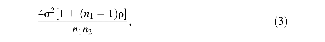
All of these elements play a crucial role, along with statistical power, in the estimation of the sample size. The statistical power is denoted as
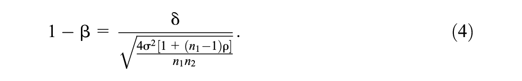
This equation shows that the power decreases as
One approach to determine the sample size is using the design effect:

which considers the effect of clustering. The total number of subjects is calculated based on the sample size obtained for an individually randomized design and then is inflated by the design effect with the fixed cluster size
An alternative approach to determine the sample size uses the factors that influence power. Moerbeek and Teerenstra (2016) presented formulas describing the relation between statistical power, effect size, Type I error rate, ICC, and sample size. Equation 4 can be rewritten so that the number of clusters becomes a function of cluster size, Type I error rate, ICC, power, and effect size:
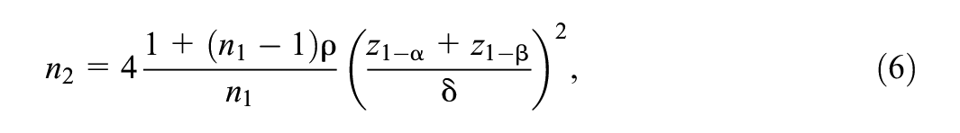
where
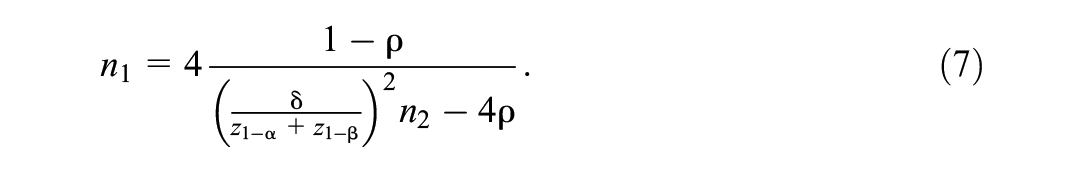
Here, it can be seen that, for a small number of clusters, the desired power level may not always be achieved, even when the cluster size increases to infinity (Hemming et al., 2011).
However, important to note that the methods for estimating the sample size discussed until now have been established for the NHST framework, which comes with notable limitations. These limitations will be explored in greater detail in the next section.
Hypothesis Testing
Limitations and Criticisms of NHST
Despite the widespread use of NHST, criticism of this approach has grown over the past few decades. Hoijtink, Mulder, et al. (2019) provide an extensive account of numerous issues associated with NHST. One criticism in their article is related to the use of the NHST approach in research. The excessive emphasis on p-values has contributed to publication bias, as studies yielding statistically significant results are more likely to be published, leading to the failed drawer phenomenon. Furthermore, this emphasis on p-values has led some researchers aiming to advance their careers to engage in questionable research practices, such as p-hacking, hypothesizing after the results are known, and cherry-picking. A second criticism is that the use of a dichotomous decision rule based on
A third criticism is the question of whether one is even interested in testing the null hypothesis. The null hypothesis indicates that there is zero effect, or in other words, that two groups have exactly the same means on a continuous outcome variable. This hypothesis is operationalized as
Beyond Null Hypothesis Testing
Diverse types of hypotheses can be of interest to researchers; to illustrate some of these types, we consider the study presented in the “CRTs” section, where Ausems et al. (2002) collected data on four treatment conditions in a smoking prevention intervention. For the sake of simplicity, in the formulation of the hypotheses, we will only use two of the treatment conditions, namely the in-school and out-of-school interventions. However, it should be noted that the hypotheses that will be presented can include more than two conditions. An informative hypothesis shows that there is an order or an expected relationship between the treatment condition means, using equality and order constraints Hoijtink (2012). This type of hypothesis is created based on the findings in the literature or the actual expectations of the researchers. In the study by Ausems et al. (2002), a possible informative hypothesis is

where the mean of the in-school smoking prevention program is expected to be larger than the mean of the out-of-school smoking prevention program. On the other hand, a hypothesis without any constraint is called an unconstrained hypothesis

Such a hypothesis implies that the researcher does not have any a priori expectations concerning the group means. A final hypothesis that is used in this article is the complement hypothesis, which, in the case of

This hypothesis covers all possible parameter values that are not covered in
Recognizing the widespread use of the null hypothesis in social sciences, and considering that the project aims to provide researchers with the necessary tools, we included the null hypothesis as a possible hypothesis of study. In this article, we provide a methodology for sample size determination for two-group comparisons. The first pair of competing hypotheses includes the equality-constrained hypothesis

while Hypothesis set 2 contains a pair of informative hypotheses:

Hypothesis set 2 can be used when one has good reason to believe one of the treatments is performing better than the other (
An example where Hypothesis set 1 clearly represents the researchers’ expectations is a study of the effect of cognitive behavioral therapy (CBT) on reducing alcohol consumption. The null hypothesis
Bayes Factor
The Bayes factor is a quantification of the relative support of the data for one hypothesis over another (Heck et al., 2022). It is also known as the ratio of two marginal likelihoods, or the marginal probability of the data

However, when comparing an (in)equality-constrained hypothesis with the unconstrained hypothesis
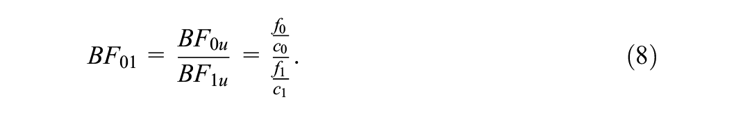
where
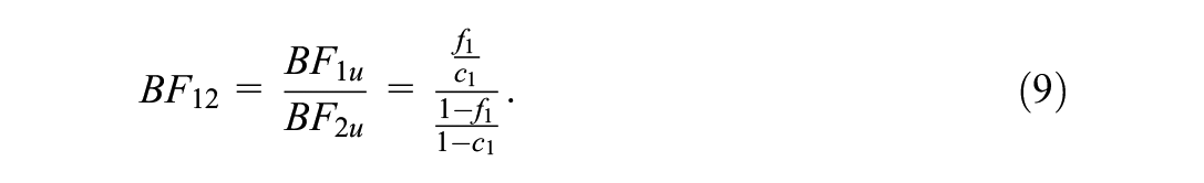
where the Bayes factor is the ratio of the Bayes factor for the informative hypothesis (
Following the Savage-Dickey density ratio, the computation of the fit and complexity of the null hypothesis (
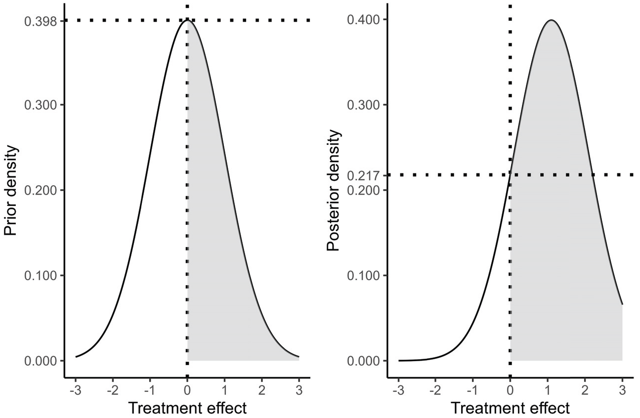
Prior and posterior distribution of the treatment effect
The present article uses the approximated adjusted fractional Bayes factor (AAFBF), which uses a fraction of the information in the data, denoted as the fraction
One of the advantages of the Bayes factor is that it is easy to interpret. Given that the Bayes factor is a quantification of the support for one hypothesis over the other, the interpretation is how much relative support the data have for one hypothesis over the other. For instance, if
Methodology for Sample Size Determination
Fu et al. (2021) proposed a method to determine the sample size using the Bayes factor for hypothesis testing. The sample size is determined by the probability (

where
The probabilities and the thresholds are specified by the researcher, taking into account the objective of the study, and they may take different values for each hypothesis in the set. In cases where the study is high-stakes and the aim is to obtain compelling evidence with high probabilities, the thresholds and the probabilities are relatively large. To illustrate, consider a study of a new medication for treating post-traumatic stress disorder. This new medication may possess severe and harmful side effects, including severe drowsiness or risk of dependency, and the costs associated with its development can be substantial. In such cases, researchers must be confident that the new medication offers clear benefits over the standard treatment by choosing high thresholds and probabilities for sample size determination, such as 10 and 0.9. This will lead to a high probability of finding a large Bayes factor. In comparison, in cases where the side effects of the treatment are less severe, researchers may opt for lower probabilities and thresholds. For instance, consider a pilot study designed to compare the effect of CBT alone with the effect of using an app with AI, developed to interact with patients with anxiety disorders, as a complement to CBT. Considering the exploratory nature of the study and the noncritical implications of using the app in conjunction with CBT, researchers may use low thresholds of, say, 3 and probabilities of .8. Furthermore, if researchers do not aim to collect more evidence for one of the hypotheses under study, we suggest maintaining the same probability and threshold for both.
As mentioned earlier, in a CRT, two sample sizes need to be determined: cluster sizes and number of clusters. The strategy proposed in this paper fixes one of the samples, with the other to be determined. The algorithm can be seen in Figure 2.
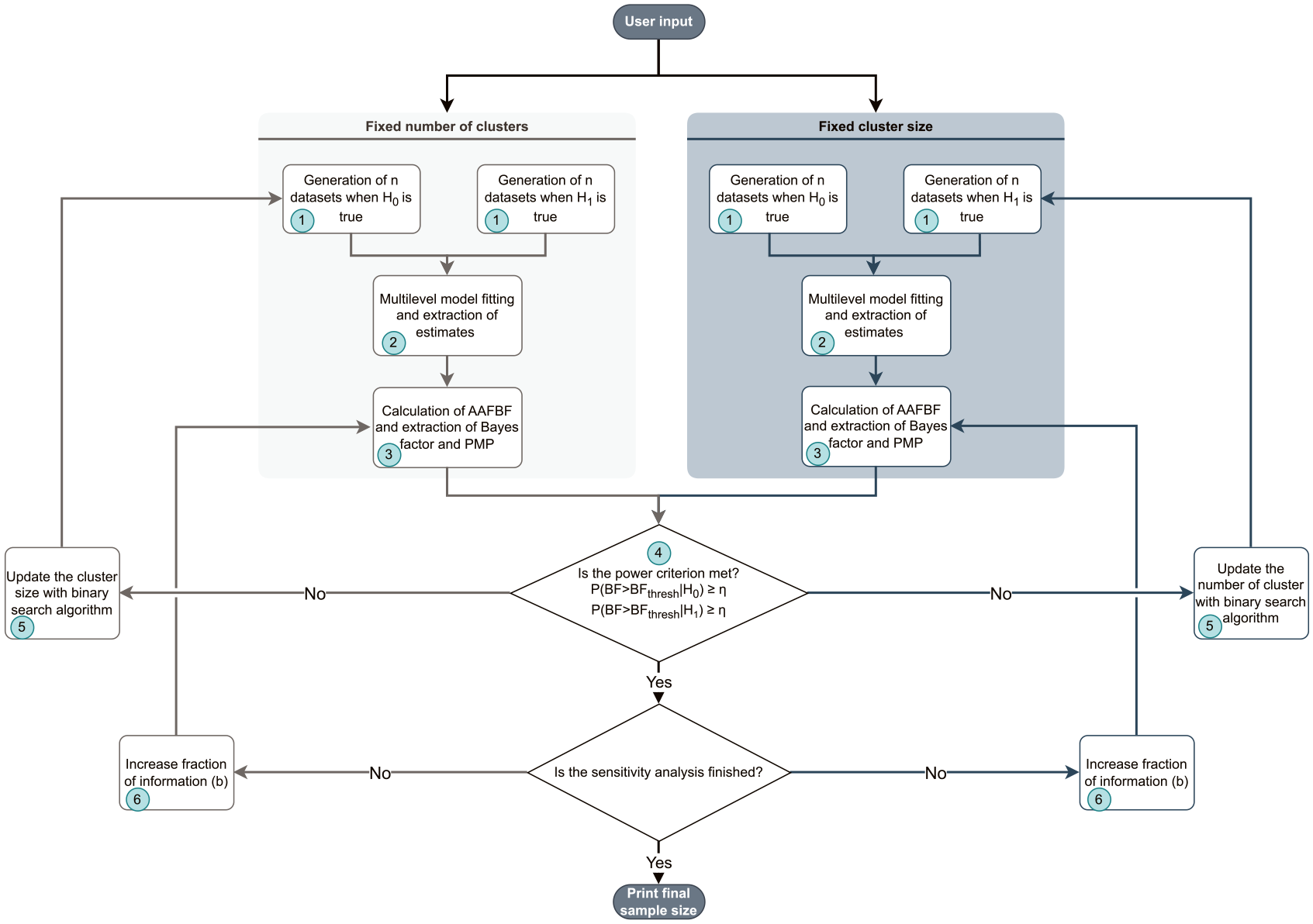
Algorithm of function for sample size determination in cluster-randomized trials when using the Bayes factor to test informative hypotheses, including the null hypothesis.
The first step in this method is to generate data sets corresponding to a two-group-parallel conditions CRT, with a given number of clusters and cluster size. The second step is to fit the multilevel model in Equation 1 to the data with the function lmer from the R package lme4 (Bates et al., 2015). The third step is to use the estimates of means and variance of the means for both treatment conditions to calculate the Bayes factors for both hypotheses in Hypotheses set 1 or 2. The fourth step is to calculate the proportion of generated data sets for which the Bayes factors exceed the threshold and to evaluate the Bayesian power criterion. The fifth step, which occurs when the power criterion in Equation 10 is not met, is to change the sample size. Rather than increasing the sample size by only one, the algorithm incorporates a binary search to efficiently find the required sample size and reduce the computation time (see Appendix B). In the case of Hypothesis set 1, a sensitivity analysis is carried out, which means that the aforementioned first five steps are repeated for different choices of fraction of information
In the repository and in the R package, two functions to determine the sample size for a trial with two parallel treatment conditions can be found. The function SSD_crt_null determines the sample size when one of the hypotheses has an equality constraint, which is the Hypothesis set 1. Meanwhile, the function SSD_crt_inform determines the sample size for Hypothesis set 2.
The arguments necessary to determine the sample size are the following:
eff_size is a numeric value corresponding to the standardized mean difference between the treatment and control conditions.
n1 is a numeric value that specifies the sizes of the clusters. All clusters are assumed to have the same size. The default value is 15 individuals in each cluster.
n2 is a numeric value that specifies the total number of clusters. The default is 30 clusters: 15 in the experimental condition and 15 in the control condition.
BF. thresh1 is a numeric value that specifies the desired minimum of the Bayes factor under the informative hypothesis
eta1 is a numeric value that indicates the probability of finding a Bayes factor equal or larger than the threshold, given that the informative hypothesis
ndatasets is a numeric value that indicates how many data sets are generated to evaluate the power criterion. The default is 5,000 data sets.
rho is a numeric value that specifies the intraclass correlation.
fixed is a string that specifies which sample size is fixed. When the number of clusters is fixed (fixed = “n2”), the function determines the cluster sizes. If the cluster sizes are fixed (fixed = “n1”), then the function determines the number of clusters. The default setting is “n2”.
max is a numeric value that indicates the maximum sample size that is used by the algorithm: if the algorithm reaches this sample size, it stops. By default, the maximum sample size is 1,000.
batch_size is a numeric value that indicates the batch size in the multilevel model fitting, which is a strategy to improve memory usage efficiency and computational performance, given that the data sets might become very large and require a considerable amount of computational effort for model fitting. The default is 100 models at the same time.
The function SSD_crt_null has the following additional arguments:
b_fract is a numeric value that specifies the maximum value that the fraction of information b is multiplied by in the sensitivity analysis. A sensitivity analysis is carried out for all integer values ranging from 1 to b_fract. This means, the fraction of information taken from the data increases from
BF.thresh0 is a numeric value that specifies the desired minimum of the Bayes factor under the null hypothesis
eta0 is a numeric value that indicates the probability of finding a Bayes factor equal or larger than the threshold, given that the null hypothesis is true. The default value is 0.8.
The outputs are different for SSD_crt_null and SSD_crt_inform. However, for both functions, the output includes the hypotheses under consideration, the sample size required, whether the number of clusters or the cluster size was fixed, the probabilities that the Bayes factor is higher than the threshold, and data sets containing the Bayes factors calculated during the simulation. For SSD_crt_null, the output also incorporates the results for different choices of b.
Simulation Study
Design
Four simulations were carried out to provide sample sizes for various realistic scenarios. Two of the simulations, one for each hypothesis set, aimed to determine the number of clusters given a fixed cluster size, while the other two aimed to determine the cluster size for a fixed number of clusters. The common factors in the design were the following:
Intraclass correlation: .025, .05, .1.
Effect size: 0, .2, .5, .8.
Bayes factor threshold: 1, 3, 5.
Probability: .8.
Maximum sample size: 1,000.
Note that we restrict to equal Bayes factor threshold and probabilities for simplicity and space limitations.
Determining the Number of Clusters
To determine the number of clusters, the cluster size was fixed to the following values:
Cluster sizes: 5, 10, 40.
Together with the factors that were common for both simulations, 81 combinations were formed. For each of these combinations, 5,000 data sets were generated.
Determining the Cluster Size
To determine the cluster sizes, the number of clusters was fixed to the following values:
Number of clusters: 30, 60, 90.
The total of formed combinations of the factors was 81, and for each of these combinations, 5,000 data sets were generated.
The minimum sample size was set inside the functions SSD_crt_null and SSD_crt_inform; for the cluster size, it was 5, and for the number of clusters, it was 6, while the maximum was set to 1,000 in the functions’ argument. The reason for using a maximum sample size was to provide a stopping point, given that with a small number of clusters, sufficient power is not always achieved, even in cases where the cluster size increases to infinity (Hemming et al., 2011). In addition, to test Hypothesis set 1, a sensitivity analysis was carried out for each combination with fractions of information
Results
Taking into account the limited space, this subsection presents a selection of the required sample sizes in tables. Readers interested in exploring additional results not displayed here can access them in the following Shiny app (https://utrecht-university.shinyapps.io/BayesSamplSizeDet-CRT/).
Determining the Number of Clusters for Hypothesis Set 1
Table 1 presents the required number of clusters and the probability of exceeding the threshold
Required Total Number of Clusters With a Fraction of Information Equal to 1 and Probability (
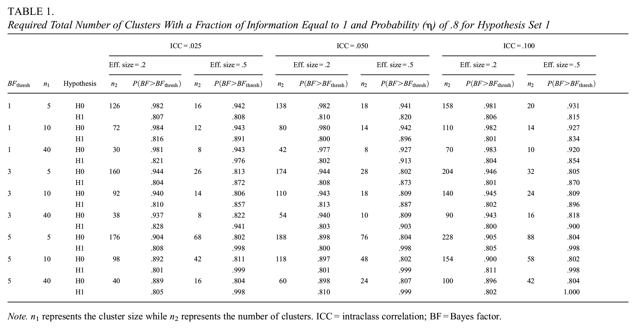
Note. n 1 represents the cluster size while n2 represents the number of clusters. ICC = intraclass correlation; BF = Bayes factor.
The results in Table 1 show that the required number of clusters to meet the power criterion increases as the ICC increases. This increase is expected, given that the higher the correlation between the individuals within a cluster, the larger the dependency among the individuals and, hence, the lower the effective sample size (Hox et al., 2017). This expectation is also possible to infer from Equation 6. Table 1 further shows a trade-off between the two sample sizes: the required number of clusters decreases if the cluster size increases. This decrease is obvious, given that the larger the cluster size, the more information is available within each cluster and, hence, fewer clusters are needed. The results also show an inverse relationship between the effect size and the number of clusters, which is not surprising, as larger effect sizes are easier to detect than smaller effect sizes. With respect to the Bayes factor threshold, the relationship with the number of clusters is proportional, meaning that increasing the threshold requires a larger number of clusters to achieve the support for the correct hypothesis.
As the reader can easily verify from our Shiny app (https://utrecht-university.shinyapps.io/BayesSamplSizeDet-CRT/), overall, the number of clusters required increases with the fraction of information
Determining the Cluster Sizes for Hypothesis Set 1
Table 2 presents the required cluster sizes as a function of the number of clusters, effect size, ICC, and Bayes factor thresholds. This table is similar in format to Table 1, but now the number of clusters rather than the cluster size appears in the second column, while the other columns show the required cluster sizes and corresponding Bayesian power.
Required Number of Individuals per Cluster With a Fraction of Information Equal to 1 and Probability (
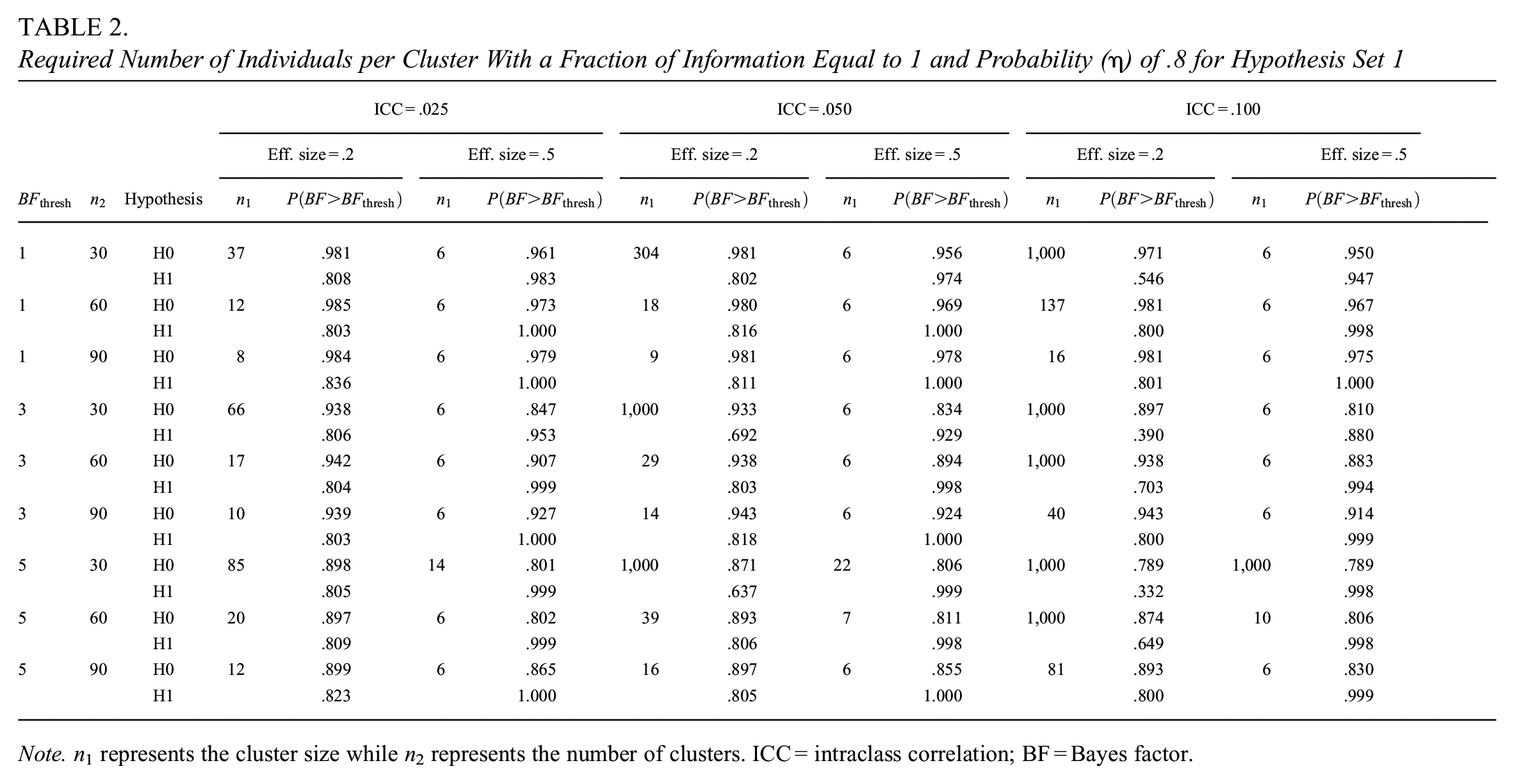
Note. n 1 represents the cluster size while n2 represents the number of clusters. ICC = intraclass correlation; BF = Bayes factor.
As shown in Table 2, the desired probability
Comparatively, when the effect size is .5, an increase in the ICC has little impact on the cluster size, and it can be seen a slight increase in the sample size under certain conditions, specifically a threshold of 5 and cluster sizes of 30 or 60. It is noteworthy that we found similar patterns of the effect of the factors we have mentioned for an effect size of .8. The reader can use the Shiny app to verify that, for an effect size of .8, cluster sizes tend to be 6 and increase slightly with the ICC under specific conditions. However, in some cases, the maximum cluster size is reached, particularly when ICC is high (
The relationship between the variables in Table 2 is similar to those described in Table 1. Larger cluster sizes are required when the effect size and the number of clusters decrease. There is a notable difference in the Bayesian power according to the effect size: with a small effect size, the increase in ICC leads to a considerable increase in cluster size.
In general, larger cluster sizes were required with increasing the Bayes factor threshold and the fraction
Determining the Number of Clusters for Hypothesis Set 2
Table 3 is different from the tables presented for Hypothesis set 1. The consideration of hypotheses with only inequality constraints requires the simulation and test for one hypothesis, given that, in this case, we are testing one hypothesis (i.e.,
Required Total Number of Clusters Condition With Probability (
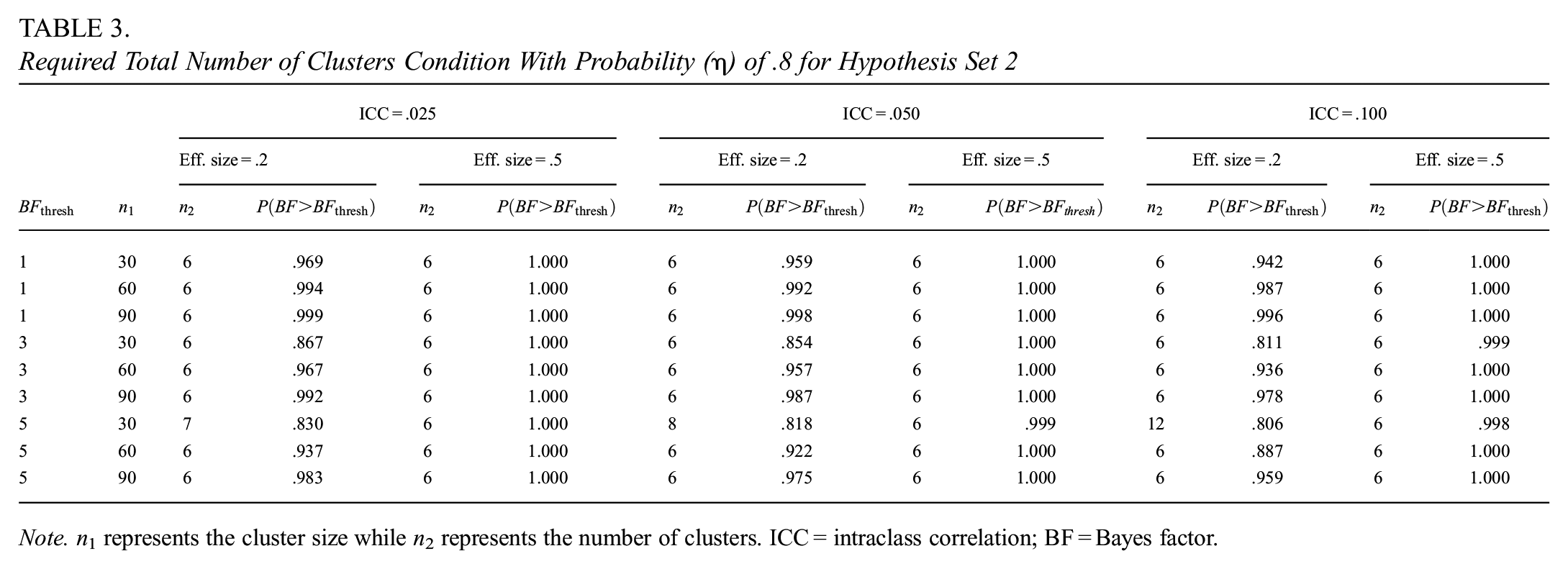
Note. n 1 represents the cluster size while n2 represents the number of clusters. ICC = intraclass correlation; BF = Bayes factor.
The results clearly indicate that, regardless of the Bayes factor threshold, ICC, effect size, and cluster size, the required total number of clusters is 6, 3 in control and 3 in treatment condition. The cases that deviate from this tendency have the largest thresholds, the smallest cluster sizes, and the smallest effect sizes. This tendency means that, while the number of clusters may be larger in specific conditions, overall, the power criterion is easily met, with a number of clusters close to the minimum specified in the design of the simulation study.
Determining the Cluster Size for Hypothesis Set 2
Table 4 presents the cluster size as a function of the number of clusters, ICC, effect sizes, and Bayes factor thresholds. From the table can be inferred that, regardless of the ICC and threshold, the required cluster size is 8 when the effect size is .5. However, in the cases where the effect size is .2, larger cluster sizes are necessary when the number of clusters is low, the ICC increases, or the threshold increases.
Required Number of Individuals per Cluster With Probability (
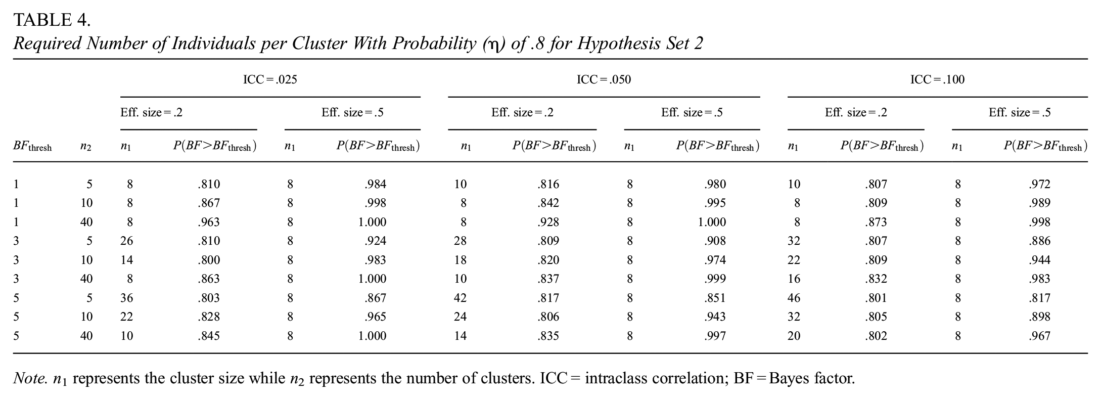
Note. n 1 represents the cluster size while n2 represents the number of clusters. ICC = intraclass correlation; BF = Bayes factor.
The comparison of the results for Hypotheses set 1 and 2 indicates that including hypotheses with equality constraints, such as
Another difference in the results of the two hypothesis sets lies in that the required sample size for Hypothesis set 2 hardly depends on the ICC, effect size, and Bayes factor threshold. The results for Hypothesis set 1 are more consistent with the effects of the factors in the frequentist framework, which are expressed in Equations 6 and 7 and proved in Moerbeek and Teerenstra (2016). Only under specific conditions, the same relationship between the factors and the sample size is observed for Hypothesis set 2, such as the smallest effect size, the largest thresholds, and the smallest fixed sample sizes.
Practical Example
This section uses the example of the CRT carried out by Ausems et al. (2002), presented above. In this study, schools were assigned randomly to four treatment conditions to evaluate two interventions and their interaction. One of the variables that was measured is the attitude toward the disadvantages of smoking, which is a result of the sum of an 11-item scale with a 5-point Likert scale, ranging from 1 = very negative to 5 = very positive.
Suppose that a researcher wants to replicate the study of Ausems et al. (2002) but is only interested in the effect of the out-of-school condition versus the control. Attitude toward the disadvantages of smoking is the outcome variable for which a power analysis is to be performed. The pair of hypotheses to consider is

The researcher performs sample size calculations. Following Moerbeek (2006), the between-cluster variance is equal to
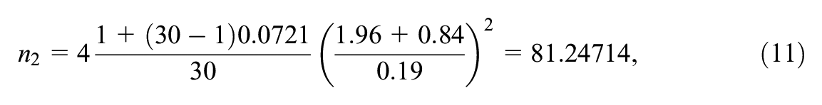
which is rounded up to 82. If the statistical power is increased to .9, the required total number of schools is
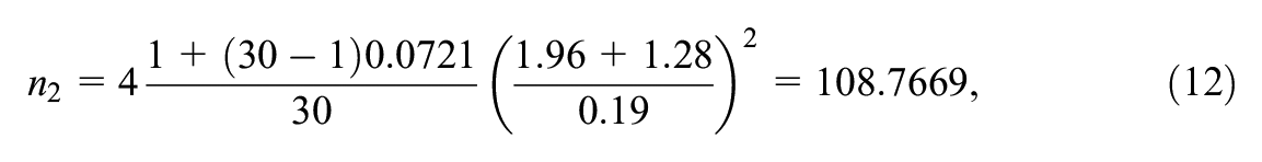
which is rounded up to 109.
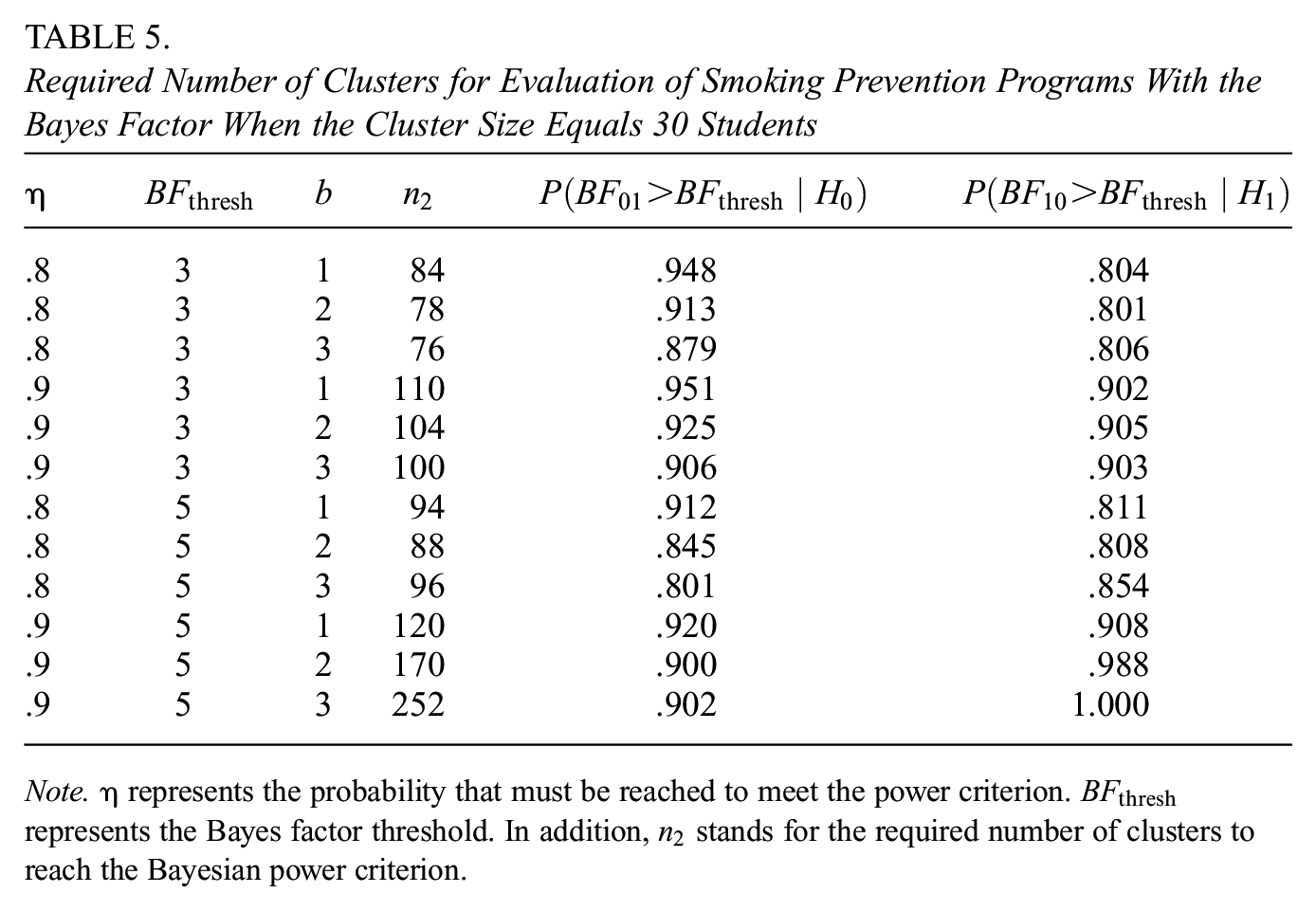
However, the researcher is also open to using the Bayes factor as a method to test the hypotheses. For this reason, the researcher performs a sample size calculation to test the hypotheses with different thresholds and probability values. Considering that the researcher wants to confirm the effects that have been studied before, the Bayes factor thresholds are 3 and 5, and the probabilities are .8 and .9.
The results presented in Table 5 demonstrate that the required number of clusters can vary from 84 up to 252, increasing with the threshold (
The original study by Ausems et al. (2002) included 143 schools, which exceeds most of the required number of schools as listed in Table 5. This implies that this study, maintaining the same number of schools, could have ensured an 80% probability that the Bayes factor would be larger than 3 or 5, as well as ensured a 90% probability of obtaining a Bayes factor larger than 3.
Required Number of Clusters for Evaluation of Smoking Prevention Programs With the Bayes Factor When the Cluster Size Equals 30 Students
Note.
Discussion
This article presents an innovative method for determining the sample size for CRTs based on Bayesian power. The method is designed to determine the number of clusters or the cluster sizes when one of them is fixed. The Bayesian power criterion specifies that the sample size is determined so that it ensures a probability (
To facilitate this approach, we have developed two functions, SSD_crt_null and SSD_crt_inform, that are implemented and freely available in an R package called SSD_Bayes_ML. The first function determines the required sample size for the evaluation of Hypothesis set 1, where
The results showed the effect of ICC, effect size, and fixed sample size on the determination of the required sample size. Larger sample sizes are required when the ICC increases, the fixed sample size is small, or the effect size is small. These results align with the effect of these same factors on the sample size determination in the frequentist approach (Moerbeek & Teerenstra, 2016; Raudenbush, 1997). The simulation also showed the trade-off between the number of clusters and cluster sizes. In addition, as anticipated (Hemming et al., 2011), the desired probability
The effects of the Bayes factor threshold and fraction of information
In comparison, our findings for Hypothesis set 2 suggest that the required sample sizes tended to be small and varied little, regardless of the factor levels used in the simulation study. This tendency lends additional support to questioning the testing of the null hypothesis (for further arguments against the use of NHST, see: Anderson et al., 2000; de Schoot et al., 2011; Gu et al., 2014; Hoijtink, Mulder, et al., 2019; Klugkist et al., 2011).
The simulations exhibited the differences in reaching the Bayesian power criterion for different hypotheses. The power criterion was easily met when evaluating Hypothesis set 2 for all conditions. Moreover, the required sample size had a small range of values and varied little, especially for cases with medium and large effect sizes. In comparison, when evaluating Hypothesis set 1, the required sample size varied considerably, and in cases with small effect sizes and a small number of clusters, the power criterion was not met, even after reaching 1,000 individuals per cluster.
Throughout the article, comparisons of this sample size determination method with that of the frequentist approach were drawn to show the differences between the two approaches, as well as highlighting the advantages of hypothesis testing with the Bayes factor. In NHST, statistical power is defined as the probability of rejecting the null hypothesis when there is a treatment effect, thus avoiding a Type II error. Researchers perform a priori power analysis or sample size calculation to ensure a certain statistical power in their studies. The methodology for sample size determination proposed here is similar in that it aims to ensure a probability; however, it goes beyond avoiding committing a Type II error. In the proposed method, we are ensuring the probability of obtaining a certain amount of relative support for a hypothesis when said hypothesis is true. In this way, although the error rate is not the primary focus of the methodology, researchers may consider
An additional advantage of the method presented in this paper is that it allows the testing of different hypotheses beyond the null hypothesis. The hypotheses of the study presented in this article are limited to the null and informative hypotheses; however, the Bayes factor can also be used to test interval hypotheses. Future research may focus on expanding the present method to test interval hypotheses, which would open the possibility to different designs such as the superiority design, non-inferiority design, and equivalence design (Heck et al., 2022). Likewise, the number of hypotheses under study may be larger than two, which can be another topic for future research and expansion of this method.
The method and the software presented in this paper implement the AAFBF, which is only one type of Bayes factor. While one of the advantages of the Bayes factor is the incorporation of prior information, for this type of Bayes factor, the user only has to indicate the fraction of information used to specify the prior distribution. However, the AAFBF is sensitive to different fractions of the sample in the case of equality-constrained hypotheses such as
Additional elements in CRT design that also influence the determination of sample size but were not considered in this study include unequal cluster sizes, uncertainty surrounding intraclass correlation, and non-inferiority and equivalence designs (Rutterford et al., 2015). Researchers considering unequal cluster sizes must be aware that in NHST, the loss of efficiency due to variation in cluster sizes has been shown to rarely exceed
In general, the methods for sample size determination require an educated guess of the ICC. Researchers may use values obtained from the literature or expert knowledge. For instance, Table 11.1 in Moerbeek and Teerenstra (2016) shows a summary of papers that report estimates of ICCs in CRTs across various scientific fields. Researchers may consider a sensitivity analysis and determine the sample size for a range of plausible values of the ICC to study the degree to which sample size depends on the ICC. Future research could further explore sample size determination when variances vary across treatment conditions.
Another consideration when utilizing the provided functions is computational cost, since our method to determine the required sample relies on simulations. In general, the minimum running time is approximately 5 minutes, while the largest running time is 35 hours. These results were obtained with a 16-core GPU with 250 GB of RAM. To improve efficiency and reduce computation time, the functions in the package employ a binary search algorithm to find the required sample size. However, it is important to highlight that the combinations with the largest running time always corresponded to the evaluation of Hypothesis set 1. Most likely, in the near future, this limitation of computational cost will be solved with the advances of technology.
Considering the growing popularity of Bayes factors for hypothesis testing in psychology (Heck et al., 2022), our method for sample size determination in CRTs is an important advance in research. We have previously discussed the disadvantages of NHST and how the Bayes factors provide an alternative approach to hypothesis testing that can avoid these disadvantages. One of the drawbacks of NHST is that, in practice, the decision to reject or maintain the null hypothesis relies on an arbitrary level of significance. To avert the same misinterpretation of the thresholds in our method, important to note is that the Bayes factor is the quantification of the evidence of the hypotheses under consideration, and it may take values from 0 to infinity. Although the thresholds used in this article are often seen in practice, we encourage the researchers to choose the thresholds based on the aimed-for degree of support.
This article introduced a method for sample size determination in CTRs tailored for hypothesis testing using Bayes factors. Moreover, we provided the practical implementation of the method through functions in the R package SSD_Bayes_ML. To our knowledge, this was the first contribution to Bayesian sample size determination for CRTs. This article is part of a larger 4-year project; in the years to come, we aim to focus on trials with more than two-treatment conditions (thereby extending the article by Fu [2022] to the multilevel setting) and cluster-randomized crossover. We also consider alternative measures for the evaluation of hypotheses, such as the Generalized Order-Restricted Information Criterion Approximation (GORICA) (Altinisik et al., 2021; Vanbrabant et al., 2020).
Footnotes
Appendix A
Appendix B
Declaration of Conflicting Interests
The author(s) declared no potential conflicts of interest with respect to the research, authorship, and/or publication of this article.
Funding
The author(s) disclosed receipt of the following financial support for the research, authorship, and/or publication of this article: This project was funded by the Netherlands Organisation of Scientific Research (NWO), grant number 406.21.GO.006.