Sage Journals: Discover world-class research

Abstract

To objectively compare groups on any latent trait using tests, the absence of differential item functioning (DIF) is crucial. While the importance of DIF has been well-established in research, the question of how to identify DIF-free items is still largely open. The fact that item difficulty is not identified from observations may explain this. Recently, DIF tests utilizing the differences between item difficulties across groups, which are identified, were proposed for the Rasch and 2-parameter logistic models. The current paper aims to extend these approaches to the polytomous case using the partial credit model. Performance of the new approach is assessed using a simulation study, and practical recommendations are made.

Keywords

item response theory partial credit model differential item functioning group comparison simulation study

To objectively compare differences in latent variables between groups, it is essential that items function the same way across these groups. In item response theory (IRT), an item functions the same way across groups if the item parameters are identical across groups. A lack of identical item parameters across groups is often referred to as differential item functioning (DIF). In the factor analytic and structural equation modeling frameworks, the same phenomenon is frequently described as measurement non-invariance (Byrne & Watkins, 2003; Van De Schoot et al., 2015).

When DIF occurs, participants of different groups with the same latent trait scores will have different probabilities of answering an item a certain way. Participants with identical latent trait scores having unequal answer probabilities are undesirable and inconvenient at best. At worst, it opens up issues of systemic discrimination against certain groups by certain tests. As an example, one could think of an aptitude test used in school placements that unfairly discriminates against participants with a migration background.

As unfair discrimination with potentially life-altering consequences is naturally not intended when constructing tests, many methods have been proposed to detect DIF in an item. IRT-based methods provide a natural way of separating between-group differences in ability from item-level DIF. For this reason, a plethora of IRT methods for testing DIF have been developed.

The most popular of these are Lord’s chi-square test (Lord, 1980), area-based methods (Kim & Cohen, 1991, 1995; Millsap & Everson, 1993), and the likelihood-ratio test (Cohen et al., 1996; Kim & Cohen, 1998; W.-C. Wang & Yeh, 2003). Unfortunately, these methods often do not achieve their stated aim of identifying which items have unequal item parameters across groups regardless of group differences in ability. The reason for this is simple. When analyzing DIF using IRT models, it is necessary to establish a common scale for the item parameters. This requires an arbitrary identification constraint to be made, such as constraining at least one item to have equal item parameters across groups or constraining the average item difficulty to be the same across groups (Bechger & Maris, 2015; Kopf et al., 2015b, 2015a). While the choice of constraint imposed is arbitrary, the results of DIF testing procedures are influenced by which constraint is chosen (Bechger & Maris, 2015).

In the approaches listed above, DIF is usually thought of as being a property of an item. However, the difficulty of an item in isolation is not an empirically identifiable property. As a consequence, the question whether a particular item shows DIF or not is not an empirical matter, as explained in detail by Bechger and Maris (2015). Essentially, this means that it is not possible to empirically establish whether any single item shows DIF or not without making additional assumptions about anchor items, such as the majority of items being DIF-free. As a consequence of this, thinking of DIF as an item property may lead to conceptually and practically problematic methods of DIF detection.

To resolve this problem, Bechger and Maris (2015) propose to focus on differential item pair functioning rather than DIF. In the approach proposed by Bechger and Maris (2015) and further developed by Pohl et al. (2017, 2020), Pohl and Schulze (2021), the differences in difficulties of item pairs, which are identifiable properties, are utilized. First, they test whether the difference between item difficulties is the same across groups for each item pair. Second, they cluster the items such that those items that have similar differences in difficulties across groups are placed in the same cluster and those that do not are placed in different clusters.

The approach by Bechger and Maris (2015) has several advantages over traditional IRT DIF testing methods. First of all, it explicitly acknowledges the non-identifiability of DIF in single items, which makes the method more theoretically sound and forces researchers to acknowledge this problem. Second, the method results in clusters of items with the task of choosing the right “DIF-free” cluster left to the researcher. Importantly, this makes researchers explicitly state their criteria for which cluster to choose. This is a desirable property, as some requirements for current DIF testing methods (e.g., at least half of all items are DIF-free and DIF does not favor one group more than the other) to function well may be less known, especially to less method-inclined researchers. This could easily lead to these methods being applied without being aware of these requirements and corresponding limitations. In addition, making researchers state their assumptions leaves other researchers free to question these assumptions and also easily see what results might have been if different clusters were designated as DIF-free. Third, the assumptions about the nature of DIF (e.g., at least half the items are DIF-free, the DIF is balanced) are moved to a later stage of the DIF testing process. While the proposed DIF methods still require assumptions about the nature of the DIF to be made, these are made when choosing a cluster that is “DIF-free.” Importantly, the process of constructing the clusters themselves does not require any assumptions about the nature of DIF. This alleviates the circularity of DIF testing (to see what kind of DIF is present, a researcher already needs to make assumptions about what kind of DIF is present, which then limits what kind of DIF can be found, which may then influence future ideas about the nature of DIF as the existing literature is affected by assumptions of current DIF testing methods). Fourth, the cluster approach results in clusters of items that function similarly, rather than DIF items and non-DIF items. This may encourage researchers to think more about why certain items function similarly, and others do not, rather than merely discarding all DIF items from the test.

While the advantages of the cluster approach are clear, as of yet, no method extending this approach to the polytomous case has been developed. Polytomous items potentially function similarly or differently on any item threshold, rather than the single difficulty parameter provided by the Rasch model or 2PL model. It is not yet clear how the presence of multiple item thresholds can best be dealt with. The current paper thus aims to develop a new cluster approach to DIF in the polytomous case utilizing the partial credit model (PCM; Masters, 1982).

The rest of the paper proceeds as follows: First, the “Cluster Approach to DIF in the Dichotomous Case” section describes the methods developed by Bechger and Maris (2015) and Pohl et al. (2021) in more detail. Second, the “DIF in Polytomous Items Under the Partial Credit Model” section describes the proposed approach to detecting DIF in polytomous items. Third, the “Simulation Study” section describes conditions and outcomes of a simulation study testing the new approach. Finally, the “Discussion” section discusses the results and provides recommendations for practical use of the method proposed in this paper.

The Cluster Approach to DIF in the Dichotomous Case

To illustrate the Bechger and Maris (2015) approach to uniform DIF in the Rasch model, we provide an example below. In Table 1, the difficulties of four hypothetical Rasch model items (i.e., items with a slope parameter set to 1) in two groups with the mean ability of both groups constrained to zero are provided.

Table 1.

Example Matrix of Item Difficulties

Item	$β_{i}^{(1)}$	$β_{i}^{(2)}$
1	0	.5
2	.5	1
3	1	2.5
4	.5	2

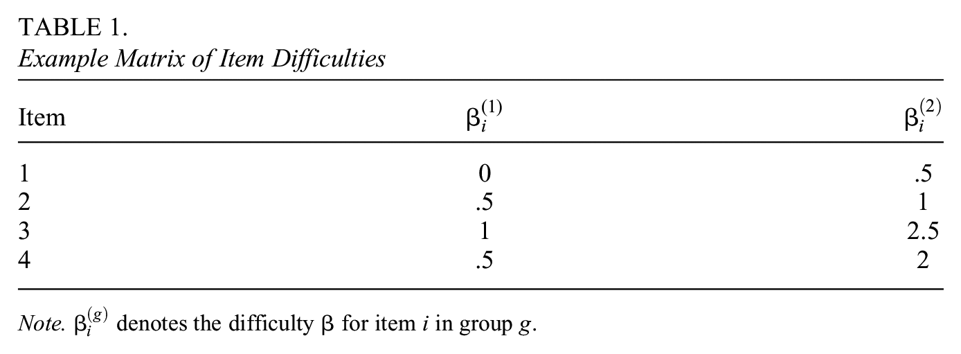
Note. $β_{i}^{(g)}$ denotes the difficulty $β$ for item $i$ in group $g$ .

Rather than directly comparing the difficulties of items across groups that are not identifiable, we instead assess the differences in difficulties of items across groups that are identifiable. Matrices of pairwise differences between item parameters per group can be constructed utilizing Equation 1:

R_{ij}^{(g)} = β_{i}^{(g)} - β_{j}^{(g)},

(1)

where $g$ denotes the group, $i$ and $j$ denote items from one to the number of items, and $R_{ij}^{(g)}$ denotes the $ij$ th entry of the $R$ matrix for group $g$ . Using the values in Table 1, this would result in the matrices $R^{(1)} = (\begin{matrix} 0 - 0.5 - 1 - 0.5 \\ 0.5 0 - 0.5 0 \\ 1 0.5 0 0.5 \\ 0.5 0 - 0.5 0 \end{matrix})$ and $R^{(2)} = (\begin{matrix} 0 - 0.5 - 2 - 1.5 \\ 0.5 0 - 1.5 - 1 \\ 2 1.5 0 0.5 \\ 1.5 1 - 0.5 0 \end{matrix})$ . Subtracting these matrices yields $Δ R = (\begin{matrix} 0 0 1 1 \\ 0 0 1 1 \\ - 1 - 1 0 0 \\ - 1 - 1 0 0 \end{matrix})$ . Note that the $Δ R$ matrix is thus a matrix of the differences of pairwise item differences over groups. A single row or column of the $Δ R$ matrix contains enough information to reconstruct the entire matrix. If all items function similarly, every entry in the $Δ R$ matrix should be close to zero. After constructing the $Δ R$ matrix, it is possible to conduct a statistical test to check whether an entry of the $Δ R$ matrix significantly differs from zero or not (Bechger & Maris, 2015). Using this statistical testing approach, clusters of items can be formed that do not differ in pairwise item differences across groups (i.e., have $Δ R$ values close to zero). In the example provided here, two clear clusters form: items 1 and 2 function similarly, and items 3 and 4 function similarly. Once the clusters are formed, the researcher can designate one of the clusters as a DIF-free cluster and perform the analyses with the items in this cluster as anchor items.

While the approach by Bechger and Maris (2015) is promising, several problems may occur. The first problem lies in the use of the statistical testing approach to forming item clusters. After all, it is possible for item 1 to not function differentially from item 2, and item 2 to not function differentially from item 3, while items 1 and 3 do function differentially. It is unclear what the clusters should be in this situation. The second potential problem is the visual approach to detecting the clusters Bechger and Maris (2015) advocate if there are no a priori expectations about the clusters. This visual approach may be difficult to implement in practice if there are many items and is difficult to test in simulation studies (Pohl et al., 2021).

For the aforementioned reasons, Pohl et al. (2021) utilize k-means clustering rather than a statistical test or utilizing visual approaches. As k-means clustering is based on the differences between the $Δ R$ values rather than the values themselves, an arbitrary row/column of the $Δ R$ -matrix can be used to cluster the items. This approach has the benefit of increased interpretability, both in empirical and simulation contexts, and resolves the scenario described above where clusters could become arbitrary. The efficacy of this approach was examined in simulation studies and compared to DIF-testing approaches, with the cluster approach performing well (Pohl et al., 2021). Notably, it was found that using the BIC as a cluster selection criterion tended to produce too few clusters. Instead, a threshold range criterion was recommended, where researchers limit to what extent item pairs can function dissimilarly while still being placed in the same cluster using a prespecified value. This value should be based on the maximum amount of item pair dissimilarity across groups a researcher is willing to tolerate (Pohl et al., 2017). Concrete recommendations on which cluster should be designated as DIF-free were made (Pohl et al., 2017), and the cluster approach was extended to the 2PL (Pohl & Schulze, 2020).

DIF in Polytomous Items Under the PCM

Equations 2 and 3 present the PCM for an item with $m$ categories and scores going from one to $m$ :

P (X_{i} = x, x > 1) = \frac{\exp \sum_{j = 1}^{x} (θ - τ_{ij})}{1 + \sum_{k = 1}^{m} \exp \sum_{j = 1}^{k} (θ - τ_{ij})};

(2)

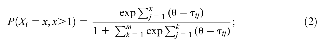
where $θ$ denotes the latent trait and $τ_{ij}$ denotes the $j$ ’th threshold of item $i$ . The probability of scoring in category one is given in Equation 3:

P (X_{i} = 1) = \frac{1}{1 + \sum_{k = 1}^{m} \exp \sum_{j = 1}^{k} (θ - τ_{ij})} .

(3)

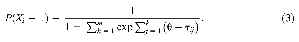
As the PCM has $m - 1$ thresholds per item, it is not straightforward to apply the approaches described above to this model. Several options for extending the existing approaches can be considered here. First, it is possible to cluster only on a single-item threshold or the average-item threshold. This approach is not ideal, as it is not clear which threshold or combination of thresholds should be chosen for this purpose, and results will differ depending on which choice is made here. Furthermore, item pairs functioning similarly on a single threshold do not guarantee the distances between this single threshold and other thresholds remain identical. Another possibility is to cluster on every item threshold present and say two items function similarly only if they function similarly to another item on every single threshold. While this approach might work, the empirically identifiable DIF properties of polytomous items described later in this paper are not used optimally by this approach. Instead, a two-stage approach is presented and advocated for in this paper.

Stage One: Equidistant Thresholds Test

To illustrate the approach in this paper, we utilize a four-category PCM item with three-item thresholds. The approach can be generalized to items with a different number of categories and generalized partial credit items, which we discuss in the discussion section. In the first stage of the approach, we are interested in establishing whether the distances between the item thresholds of a single item are the same across groups. A violation of this property would mean that a specific item has DIF. Note that while for dichotomous items DIF of a single item is not an identifiable property, the violation of equidistant thresholds is. To test for equidistant thresholds in a four-category item with three-item thresholds, the means of groups 1 and 2 are constrained to zero. We can test for equidistant thresholds by testing whether $(τ_{i 2}^{(1)} - τ_{i 1}^{(1)}) - (τ_{i 2}^{(2)} - τ_{i 1}^{(2)}) = 0$ and $(τ_{i 2}^{(1)} - τ_{i 3}^{(1)}) - (τ_{i 2}^{(2)} - τ_{i 3}^{(2)}) = 0$ utilizing a multivariate Wald test. The formula to calculate the test statistic for these two tests simultaneously is depicted in Equation 4,

ET T_{stat} = {(C \hat{τ})}^{T} {(CS C^{T})}^{- 1} (C \hat{τ}),

(4)

where $C$ is the constraint matrix $[\begin{matrix} - 1 1 1 - 1 0 0 \\ 0 0 1 - 1 - 1 1 \end{matrix}]$ ; $\hat{τ}$ is the column vector of the maximum likelihood estimates of $τ_{i 1}^{(1)}$ , $τ_{i 1}^{(2)}$ , $τ_{i 2}^{(1)}$ , $τ_{i 2}^{(2)}$ , $τ_{i 3}^{(1)}$ , $τ_{i 3}^{(2)}$ ; and $S$ is the estimated variance-covariance matrix of the aforementioned $τ$ -parameters (Pustejovsky, 2023). Note that the number of columns of this matrix is, in general, equal to the number of categories minus 1 ( $m - 1)$ multiplied by the number of groups (2). Concerning rows, every category added increases the number of rows by one (as an additional constraint is necessary). Under the null hypothesis $(C \hat{τ}) = 0$ , the equidistant threshold test (ETT) statistic asymptotically follows a chi-square distribution with one degree of freedom per constraint imposed (e.g., two degrees of freedom in the case with four categories and two groups). Items that fail the ETT must have some type of DIF, assuming the model is correctly specified (i.e., no unmodeled response styles, no non-fitting IRT model, etc.) and no type I error is made. Following this approach will thus result in a set of items that fail the test and should be eliminated from further testing, and a group of items that pass the test. Note that passing this test is not by itself sufficient to conclude that two items function similarly. After all, all thresholds of the item could be shifted by a constant in one of the groups. The second stage of the procedure eliminates this possibility.

Stage Two: Forming Item Clusters

To establish whether items that pass the ETT function similarly to other items or not, we extend the cluster approach from Pohl et al. (2021). First, we fit the model with all items that passed the ETT having the distances between item thresholds constrained to be equal across groups and the means of groups 1 and 2 constrained to zero.¹ Note that imposing these constraints induces positive covariances between the item parameters of different groups, which reduces the standard error of the $Δ R$ values we calculate later. The stages are thus best done in the order they are presented here. Using the item parameters obtained when fitting the model, we construct the $Δ R$ matrix for a single-item threshold (for the 4-category item, we will use the second threshold). This is equivalent to using all thresholds at once since the distances between thresholds are constrained to be equal across groups. The $Δ R$ matrix is constructed as $(τ_{i 2}^{(1)} - τ_{k 2}^{(1)}) - (τ_{i 2}^{(2)} - τ_{k 2}^{(2)})$ , where $i$ and $k$ are iterators from 1 to the number of items that passed the first stage. Note that it is only possible to use this single clustering on an item threshold to conclude items function similarly due to previously establishing equidistant thresholds across groups for the items. Finally, finding that items function similarly is not exactly the same as proving the items do not have DIF in the traditional sense; it could also be that all item thresholds of all items in the cluster are shifted by a single constant in one of the groups.

The clustering described above could be accomplished using various methods. In this paper, following Pohl et al. (2021), we chose to cluster items by conducting k-means clustering on an arbitrary row/column of the $Δ R$ matrix using the Ckmeans.1d.dp package (H. Wang & Song, 2011). The clustering described here is different from typical clustering scenarios for two reasons. First of all, the clustering is done on univariate data with only a small sample size (the number of items). Secondly, the $Δ R$ -matrix consists of the estimates of the differences between the item threshold differences. Depending on the standard errors of the original $τ_{i 2}^{(g)}$ estimates and the covariances between these estimates, the $Δ R$ -values can be quite uncertain. We chose to use k-means clustering method here as its effectiveness was previously established by Pohl et al. (2021).

As a final step in the clustering process, one of the clusters that form needs to be designated as the DIF-free cluster. While several approaches to this problem are possible, all of these do again involve bringing in some outside information or assumptions about the items, same as the traditional DIF-testing methods. In fact, designating the cluster with most items as the DIF-free cluster would make this method similar to traditional DIF testing methods (Pohl et al., 2021). Nevertheless, we believe the conceptual and practical advantages of this method described earlier, including its flexibility in which clusters are designated as DIF-free, still make this method a worthwhile development over traditional methods. Alternative methods of choosing a cluster are described in the discussion.

Empirical Example

To illustrate how an application of the approach to real data would proceed, an empirical example is provided. We utilize a multigroup dataset with four-category items obtained from the Program for International Student Assessment (PISA), a well-known and publicly accessible source for multigroup data (OECD, 2000). We used the reading attitude scale from PISA 2009 (OECD, 2010). The scale has eleven four-category items, for example, “I read only if I have to” (reverse coded) and “I like talking about books with other people.” The response options were “Strongly disagree,”“Disagree,”“Agree,” and “Strongly agree,” with higher scores indicating higher levels of reading enthusiasm once the reverse-coded items are considered. All code utilized in this example is available in online Supplemental Materials (available in the online version of the journal) and on https://osf.io/mfqkg/, and the data is freely accessible on the PISA website.

For the purposes of this example, we chose to examine Latvia (N = 4,502) and Serbia (N = 5,523). These groups were preferred over other countries for several reasons. First of all, the countries did not eliminate too many items in the ETT stage of the item similarity test. Second, the countries showed an interesting pattern in the clustering stage of the item similarity test, with multiple clusters of different sizes forming. It is important to note here that we chose this specific example to illustrate the approach best; we do not make any claims about its generalizability.

As a first step in the analysis, we estimated the PCM model with the means of the latent variable in both groups fixed to 0 for identification purposes. With these constraints, the average item thresholds were [−1.88, −0.30, 2.00], indicating somewhat balanced item thresholds. The values for the ETT statistics calculated using Equation 4 can be found in Table 2. Items exceeding the critical value of 5.99 based on a chi-square distribution with two degrees of freedom and a type I error rate of 0.05 are marked in bold. In addition to the ETT statistic, the difference in distances across groups is contained in the table.

Table 2.

Results of the ETT

Item	1	2	3	4	5	6	7	8	9	10	11
$d_{i 1}^{(1)} - d_{i 1}^{(2)}$	−0.20	−0.12	0.11	0.13	0.11	0.28	−0.42	−0.35	0.26	−0.03	0.37
$d_{i 2}^{(1)} - d_{i 2}^{(2)}$	−0.08	0.15	−0.05	−0.03	0.05	0.43	0.00	−0.10	0.07	−0.06	0.35
$ET T_{stat}$	3.74	5.92	2.54	2.11	1.39	22.70	26.28	13.90	3.71	0.44	18.82

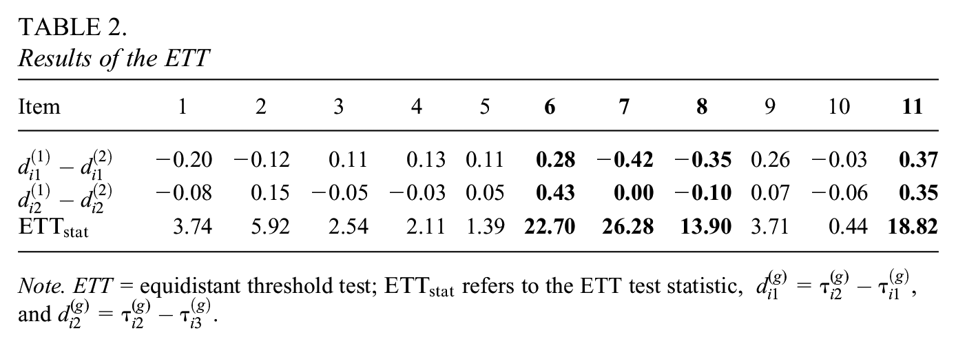
Note. ETT = equidistant threshold test; $ET T_{stat}$ refers to the ETT test statistic, $d_{i 1}^{(g)} = τ_{i 2}^{(g)} - τ_{i 1}^{(g)}$ , and $d_{i 2}^{(g)} = τ_{i 2}^{(g)} - τ_{i 3}^{(g)}$ .

As can be seen in Table 2, items 6, 7, 8, and 11 are found to have non-eq5 thresholds. After determining items 6, 7, 8, and 11 items do not pass the ETT, we run the reparametrized PCM model with the latent trait means of both groups fixed to zero. The distance parameters of the items that did not fail the ETT are constrained to be equal across groups.

To illustrate the 0.2 threshold range approach (Pohl et al., 2021) using the Ckmeans.1d.dp package, all $Δ R$ -values are displayed in the second row of Table 3. We calculate the range of a cluster as the distance between the maximum and minimum $Δ R$ -values in a given cluster. For the single cluster solution where all items are in the same cluster, this results in a range of $0 + 0.60 = 0.60$ . As this value exceeds 0.2, we add an additional cluster and recalculate the range values of the new clusters. Now, cluster 1 contains all items except item 5, which forms a cluster by itself. The cluster range value for cluster 1 is $0 + 0.23 = 0.23$ , and the cluster range value of cluster 2 is $- 0.60 + 0.60 = 0$ . Naturally, the “cluster range” of a cluster containing only one item is always zero. As the cluster range of cluster 1 still exceeds the value of 0.2, we add a third cluster. Now, items 1, 2, 4, and 10 are in cluster 1, cluster 2 still only contains item 5, and cluster 3 contains items 3 and 9. The cluster ranges are calculated as $0 + 0.08 = 0.08$ for cluster 1, $- 0.60 + 0.60 = 0$ for cluster 2, and $- 0.17 + 0.23 = 0.06$ for cluster 3. As all cluster ranges are below 0.2, we stop adding additional clusters. The final cluster solution is displayed in Table 3. A second example going into more detail on the clustering step of the approach is provided in Supplemental Material B, in the online version of the journal.

Table 3.

$Δ R$ Values and Final Cluster Assignment for the Items

Item	1	2	3	4	5	9	10
$Δ R$	0	−.08	−.18	−.06	−.60	−.23	−.08
Cluster	1	1	3	1	2	3	1

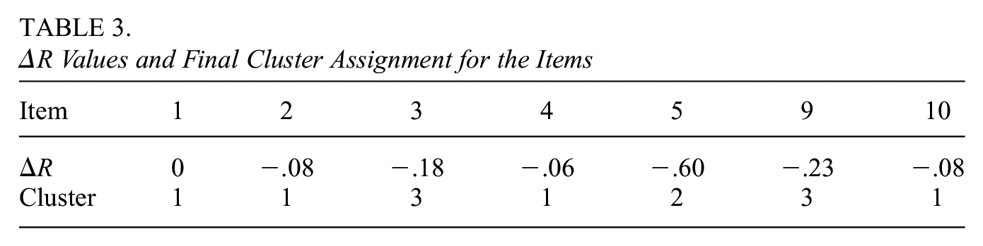
As can be seen in Table 3, items 1, 2, 4, and 10 function similarly, items 3 and 9 function similarly, and item 5 does not function similarly to any other item. As a final step in the analysis, a researcher must choose a cluster of items to be designated as DIF-free or utilize model averaging. The choice of cluster can be based on various criteria. Most current DIF testing methods utilize the principle that the largest cluster is the DIF-free cluster, but a researcher may also base their conclusion on content expertise or other grounds. The items in the designated DIF-free cluster are used as anchor items and have their item thresholds constrained to be equal across groups.

To illustrate the impact of utilizing different clusters as DIF-free on the latent trait means of the groups, we discuss the various conclusions depending on which cluster is designated as DIF-free. Note that the mean of Serbia ( ${\hat{μ}}_{Serbia}$ ) can be interpreted as the mean difference between Serbia and Latvia. If we choose to utilize cluster 1, participants from Serbia do not significantly differ from participants in Latvia in terms of mean reading enthusiasm ( ${\hat{μ}}_{Serbia} = 0.007, SE = 0.030)$ . If we choose to utilize cluster 2, participants from Serbia show substantially more reading enthusiasm than participants from Latvia ( ${\hat{μ}}_{Serbia} = 0.544, SE = 0.039)$ . If we choose to utilize cluster 3, participants from Serbia show moderately more reading enthusiasm than participants from Latvia ( ${\hat{μ}}_{Serbia} = 0.148, SE = 0.034)$ . This demonstrates the importance of choosing a cluster on well-reasoned and openly disclosed grounds when attempting to discern differences between groups.

Simulation Study

To best assess the performance of the proposed method, we first examine the performance of both stages separately. Second, we evaluate the performance of the two stages combined. All code is available in Supplemental Material (available in the online version of the journal) and on https://osf.io/mfqkg/.

Conditions and Outcomes for the Equidistant Thresholds Test

All data in this simulation study were generated using R 4.2.2 (R Core Team, 2022), and all conditions were replicated 500 times. First, data were generated for two groups, where both groups had a latent trait distributed $N (0, 1)$ . These participants answered 20 PCM items with four categories and item thresholds of $[- 1 + m, 0 + m, 1 + m]$ , where $m ~ N (0, {0.25}^{2})$ or $m ~ N (0.5, {0.25}^{2})$ were generated for each replication. The $m$ -value was added to the item thresholds to increase ecological validity (i.e., to ensure not all items have exactly the same item parameters, as this would not occur in a real test). The mean of the $m$ -values was varied across conditions to assess the performance of the test when items were not perfectly suited to the ability level of participants (i.e., there is less information). Note that based on these item thresholds, the distance between $τ_{i 2}^{(g)}$ and $τ_{i 1}^{(g)}$ is 1 and the distance between $τ_{i 2}^{(g)}$ and $τ_{i 3}^{(g)}$ is −1. To identify the model, the means of group 1 and group 2 were constrained to zero during estimation. All models were fit using the mirt R package (Chalmers, 2012), which results in marginal maximum likelihood estimates of all parameters. Sample size per group varied between 1,000, 2,000, and 4,000 to provide a good overview of power for various sample sizes.

In the generated data, the proportion of items with equidistant thresholds was kept constant at 0.5 to ensure that we have the same number of DIF and non-DIF observations to base our outcome estimates on. Non-eq6 thresholds were induced by adding a value $D$ to the distance between $τ_{i 2}^{(g)}$ and $τ_{i 1}^{(g)}$ , and subtracting the value $D$ from the distance between $τ_{i 2}^{(g)}$ and $τ_{i 3}^{(g)}$ . These non-equidistant thresholds mimic an outward threshold shift one might observe when an extreme response style is present (Jin & Wang, 2014). The $D$ -value was set to 0.25 or 0.5 depending on the condition. We varied the $D$ -value as we expected smaller $D$ -values to be more difficult to detect than larger $D$ -values. In total, this resulted in 2 (item threshold distributions) × 3 (sample sizes) × * 2 ( $D$ -values) = 12 conditions for the ETT.

As outcome measures, the type I error ( $α$ ; the item does have equidistant thresholds but is flagged as not having equidistant thresholds by the test) and power ( $1 - β$ ; the item does not have equidistant thresholds and is flagged as such) are of interest. As the base rate is known (0.5), the full contingency table can be recalculated from these results.

Results for the Equidistant Thresholds Test

As can be seen in Table 4, the power to detect non-equidistant thresholds is generally quite high. Only when the sample size per group is 1,000 and the $D$ -value is small does power fall below 0.8. Clear effects of the factors are visible, with larger $D$ -values and larger sample sizes per group making it easier is to detect non-equidistant thresholds. Varying the mean $m$ -value does not seem to affect the power much. The type I error remains constant around 0.05, regardless of condition.

Table 4.

Results for the $multivariate equidistant thresholds test$ based on 500 replications

$N$	$μ_{m}$	$D$	$1 - β$	$α$
1,000	0	0.25	.60	.05
		0.5	1.00	.05
	0.5	0.25	.58	.05
		0.5	.99	.05
2,000	0	0.25	.89	.05
		0.5	1.00	.05
	0.5	0.25	.88	.04
		0.5	1.00	.05
4,000	0	0.25	1.00	.05
		0.5	1.00	.05
	0.5	0.25	.99	.05
		0.5	1.00	.05

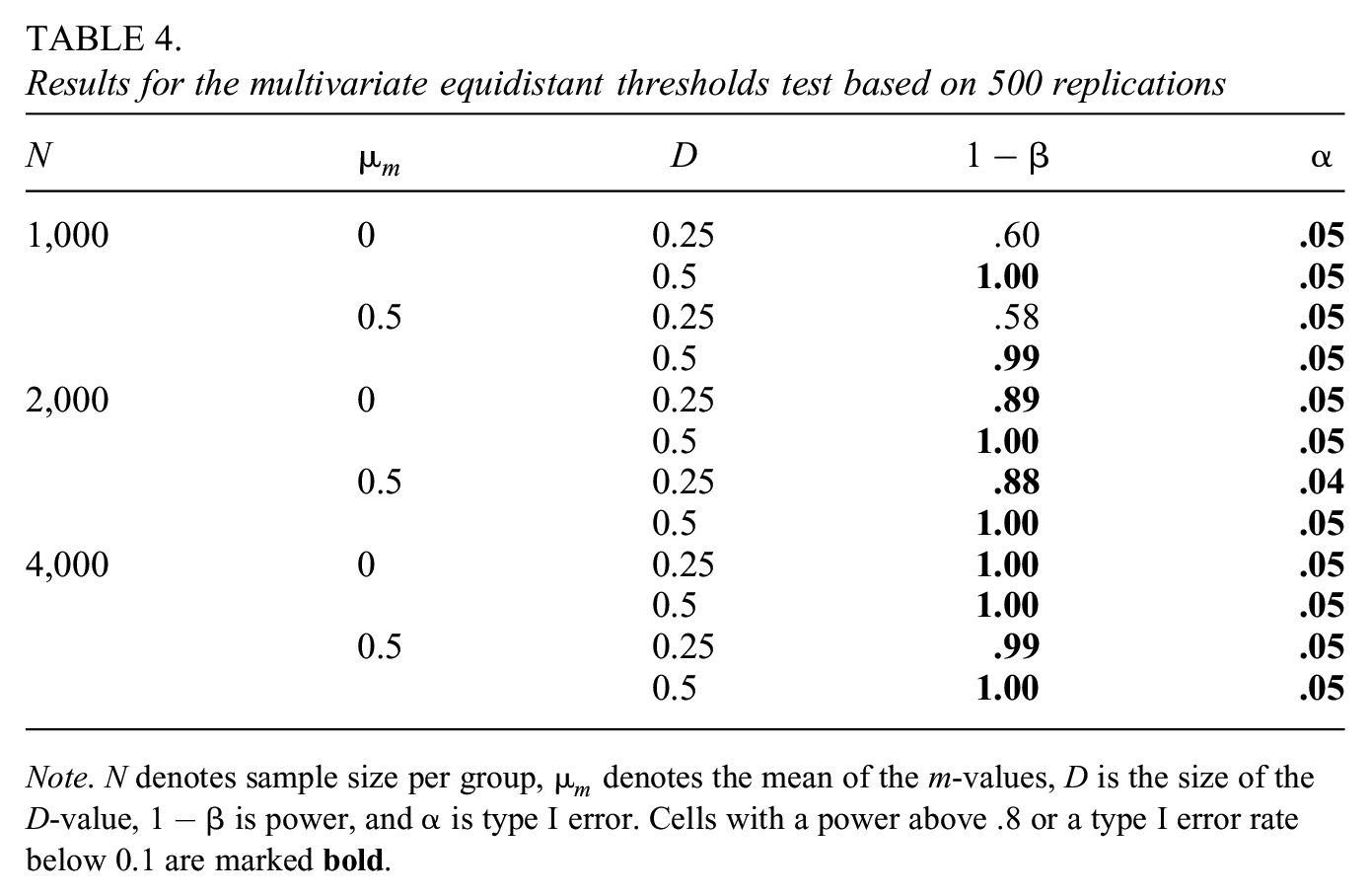
Note. N denotes sample size per group, $μ_{m}$ denotes the mean of the $m$ -values, $D$ is the size of the $D$ -value, $1 - β$ is power, and $α$ is type I error. Cells with a power above .8 or a type I error rate below 0.1 are marked bold.

Conditions and Outcomes for the Forming of Item Clusters

Conditions for the clustering simulation largely follow the conditions for the ETT simulation. Item thresholds, sample sizes, and identification constraints were identical to the ETT study. Three major changes were made to the simulation design. First, we now drop the $D$ -value and instead subtract an $E$ -value from all threshold parameters of dissimilar items in group 2 to induce dissimilarity between items. The $E$ -value was varied between 0.25 and 0.5 across conditions. Note that this item dissimilarity (unlike the one obtained by using $D$ -values) can equivalently be seen as uniform DIF (all item thresholds shifted by a constant but equal slopes across groups) in the traditional DIF framework. Second, the percentage of items with dissimilar $τ_{ij}^{(2)}$ parameters were varied between 40% and 80%. This was done since traditional methods struggle to function in conditions where a higher percentage of DIF items is present. Third, the number of DIF clusters was varied between 1 and 2 to assess whether the method performs adequately even if multiple DIF clusters are present. If there was only a single DIF cluster, the $E$ -value was added to the $τ_{ij}^{(2)}$ of all items in the DIF cluster. If there were two DIF clusters, the $E$ -value was added to half of the items in the DIF cluster $τ_{ij}^{(2)}$ values and subtracted from the other half of the DIF cluster items $τ_{ij}^{(2)}$ values. This created 2 (E-value) * 2 (item threshold distribution) × 3 (sample size) × 2 (percentage of dissimilar items) × 2 (number of DIF clusters) = 48 conditions for the clustering test.

Concerning the outcome measures of the cluster approach, we were most interested in how well the DIF-free cluster was recovered. We thus chose to label the cluster with the most DIF-free items as the focal cluster, similar to Pohl et al. (2021), and examine outcomes related to this cluster. We chose the false positive rate (FPR, the rate of items that do belong in the focal cluster but are not placed there by the clustering) and true positive rate (TPR, the rate of items that do not belong in the focal cluster and are not placed there) as outcomes. In addition, we were interested in two further outcomes. First, the number of clusters formed was of vital importance. If the number of clusters formed is too high, the eventual step of designating a cluster as a non-DIF cluster that has to be made by the researcher would become needlessly complex and prone to error. Finally, we considered the specificity (the proportion of items in the focal cluster that are DIF-free/similar items) to be of interest. Specificity is relevant here for two reasons. First of all, the focal cluster should contain as few DIF items as possible to prevent misestimation of the latent trait. Second, a researcher may wish to apply traditional DIF techniques to their selected non-DIF cluster. In order for these techniques to be effective, a specificity above 0.5 may be required (Woods, 2009).

Results for the Forming of Item Clusters

Note that several approaches for selecting the number of clusters were considered. As the 0.2 threshold range approach showed high TPR rates even in lower sample size conditions, we display results based on this criterion in Table 5. Results for threshold range approaches of 0.4 or 0.6 and the BIC for selecting a number of clusters can be found in Supplemental Material A (available in the online version of the journal).

Table 5.

Clustering Results for the Threshold Range Criterion of 0.2 Based on 500 Replications

$N$	$μ_{m}$	% DIF	$E$	$N_{c}$	TPR	FPR	Specificity	$\hat{N_{c}}$
1,000	0	40	0.25	2	0.99	0.10	0.99	2.38
				3	0.99	0.10	0.99	3.23
			0.5	2	1.00	0.13	1.00	2.62
				3	1.00	0.15	1.00	3.57
		80	0.25	2	0.98	0.03	0.94	2.36
				3	0.98	0.04	0.93	3.28
			0.5	2	1.00	0.02	1.00	2.60
				3	1.00	0.02	1.00	3.45
	0.5	40	0.25	2	0.99	0.13	0.99	2.44
				3	0.99	0.10	0.99	3.23
			0.5	2	1.00	0.12	1.00	2.63
				3	1.00	0.13	1.00	3.57
		80	0.25	2	0.97	0.04	0.93	2.41
				3	0.97	0.07	0.91	3.38
			0.5	2	1.00	0.03	1.00	2.63
				3	1.00	0.02	1.00	3.51
2,000	0	40	0.25	2	1.00	0.01	1.00	2.03
				3	1.00	0.01	1.00	3.01
			0.5	2	1.00	0.01	1.00	2.04
				3	1.00	0.00	1.00	3.02
		80	0.25	2	1.00	0.00	0.99	2.03
				3	1.00	0.00	1.00	3.01
			0.5	2	1.00	0.00	1.00	2.04
				3	1.00	0.00	1.00	3.02
	0.5	40	0.25	2	1.00	0.01	1.00	2.04
				3	1.00	0.01	1.00	3.02
			0.5	2	1.00	0.01	1.00	2.05
				3	1.00	0.01	1.00	3.03
		80	0.25	2	1.00	0.00	0.99	2.04
				3	1.00	0.00	0.99	3.02
			0.5	2	1.00	0.00	1.00	2.04
				3	1.00	0.00	1.00	3.05
4,000	0	40	0.25	2	1.00	0.00	1.00	2.00
				3	1.00	0.00	1.00	3.00
			0.5	2	1.00	0.00	1.00	2.00
				3	1.00	0.00	1.00	3.00
		80	0.25	2	1.00	0.00	1.00	2.00
				3	1.00	0.00	1.00	3.00
			0.5	2	1.00	0.00	1.00	2.00
				3	1.00	0.00	1.00	3.00
	0.5	40	0.25	2	1.00	0.00	1.00	2.00
				3	1.00	0.00	1.00	3.00
			0.5	2	1.00	0.00	1.00	2.00
				3	1.00	0.00	1.00	3.00
		80	0.25	2	1.00	0.00	1.00	2.00
				3	1.00	0.00	1.00	3.00
			0.5	2	1.00	0.00	1.00	2.00
				3	1.00	0.00	1.00	3.00

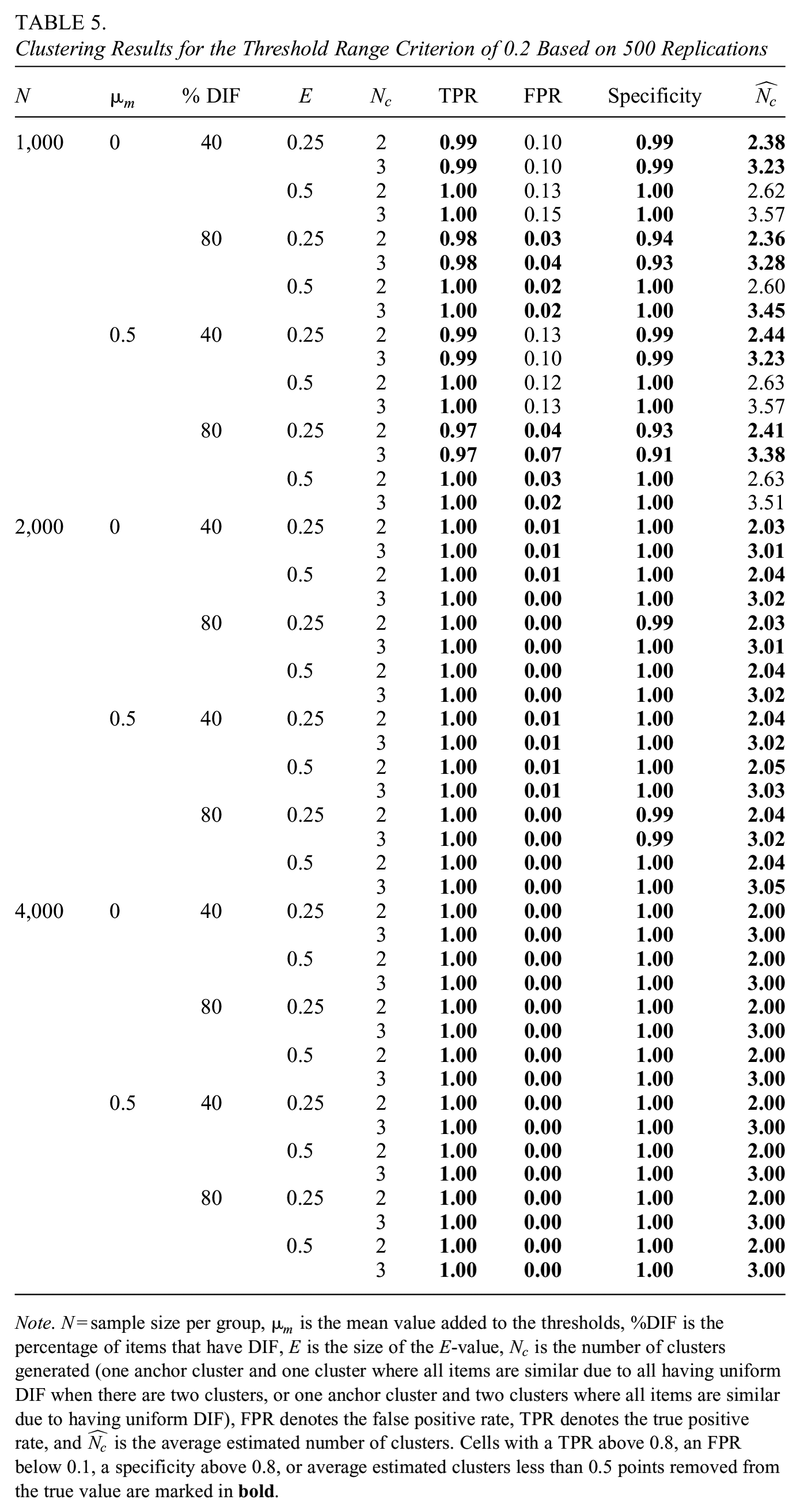
Note. N = sample size per group, $μ_{m}$ is the mean value added to the thresholds, %DIF is the percentage of items that have DIF, $E$ is the size of the $E$ -value, $N_{c}$ is the number of clusters generated (one anchor cluster and one cluster where all items are similar due to all having uniform DIF when there are two clusters, or one anchor cluster and two clusters where all items are similar due to having uniform DIF), FPR denotes the false positive rate, TPR denotes the true positive rate, and $\hat{N_{c}}$ is the average estimated number of clusters. Cells with a TPR above 0.8, an FPR below 0.1, a specificity above 0.8, or average estimated clusters less than 0.5 points removed from the true value are marked in bold.

As can be seen in Table 5, the threshold range criterion of 0.2 generally has a high TPR in all conditions. Since the TPR is always near 1, the effect of factors is difficult to distinguish here.

The high power at lower sample sizes does come at the cost of an inflated FPR when the sample size is 1,000 participants per group. This inflated FPR is particularly pronounced when the percentage of DIF items is low. This seemingly contradictory behavior can be explained by the fact that as the number of anchor items increases, it becomes more and more likely that the most extreme anchor items are not within a $Δ R$ range of .2 of each other. If this is the case, multiple clusters containing anchor items would be formed, inflating the FPR. This problem disappears when the sample size is increased to 2,000 participants per group, which reduces the standard error of the $Δ R$ values. Overall, the FPR increases when the number of DIF clusters is higher or when the $E$ -value is higher, but only when the sample size is below 2,000.

Due to the high power, the specificity of the focal cluster is often close to 1 and remains above 0.9 in all conditions. Smaller $E$ -values, higher numbers of DIF clusters, and higher percentages of DIF items somewhat decrease the specificity, but only to a small extent and in combination with a sample size below 2,000.

In terms of the average number of estimated clusters ( $\hat{N_{c}}$ ), the 0.2 threshold range approach tends to create slightly more clusters than are truly present when the sample size is 1,000 participants per group. Several factors seem to impact the $\hat{N_{c}}$ . As one might expect, a higher number of real clusters leads to a higher $\hat{N_{c}}$ . In addition, higher $E$ -values lead to a higher $\hat{N_{c}}$ when the sample size is lower, as the DIF clusters are more easily recognized. Higher sample sizes lead to an $\hat{N_{c}}$ closer to the real number of clusters. This decrease in the $\hat{N_{c}}$ is likely driven by the standard error of the $Δ R$ -values of all items being reduced, which leads to easily distinguishable clusters and lower FPR as discussed earlier. Lastly, the percentage of DIF items and the mean $μ_{m}$ value do not seem to have a strong impact on the $\hat{N_{c}}$ .

Conditions and Outcomes for the Combined Approach

Finally, we were also interested in showcasing a combination of the ETT and cluster methods, as would be done in practice. As a full factorial design here would lead to a very high number of conditions and an inaccessibly large set of results, we chose to instead showcase some specific conditions as an illustration.

First of all, conditions where there is no DIF present were considered to evaluate the FPR rate of the proposed full approach. Item thresholds and sample sizes were generated identically to previous conditions. No $D$ or $E$ values were added to any of the items, resulting in $2$ (item threshold distributions) × 3 (sample sizes) $= 6$ conditions.

Second, the performance of the ETT and clustering combined was evaluated in the presence of both types of DIF. As the performance of the ETT and cluster approaches separately is already examined in the previous conditions, we were particularly interested in conditions where the ETT does not perform optimally. This enabled us to observe whether a less successful ETT adversely affects the subsequent clustering. We thus chose three conditions where the ETT did not perform well in terms of power: A sample size of 1,000 with a mean $m$ -value of 0 and a $D$ -value of 0.25, a sample size of 1,000 with a mean $m$ -value of 0.5 and a $D$ -value of 0.25, and a sample size of 2,000 with a mean $m$ -value of zero and a $D$ -value of 0.25.

When examining the performance of the combined approach, it is important to keep in mind that eliminating items due to failing the ETT will reduce the effective sample size of the cluster stage (i.e., the number of items that can be clustered). We thus wanted to ensure that any potentially observed reduction in clustering performance was due to “contaminated” non-ET items making it into the cluster stage rather than a reduction in the effective clustering sample size. We, therefore, added two extra conditions where the ETT performed well: A sample size of 1,000 with a mean $m$ -value of zero and a $D$ -value of 0.5, and a sample size of 2,000 with a mean $m$ -value of zero and a $D$ -value of 0.5.

As all five aforementioned ETT results concern conditions where half of the items had non-eq7 thresholds, we chose to again induce non-equidistant thresholds in half of the items. In addition, 12 of the items were designated as dissimilar by subtracting (and adding in the case of multiple dissimilar item clusters) an $E$ -value. The items that had an $E$ -value added or subtracted were spread equally over the equidistant threshold items and the non-equidistant threshold items. We varied the $E$ -value between 0.25 and 0.5, as this had a large impact on the efficacy of the clustering. The number of dissimilar item clusters also varied between one and two. This resulted in $5$ (number of selected conditions) × 2 (E-values) × 2 (number of dissimilar item clusters) = 20 conditions in addition to the six conditions without DIF.

Concerning the outcome measures of the combined approach, we distinguish between the conditions where no DIF is present and the conditions where DIF is present. In the no DIF conditions, we were interested in the FPR and the number of clusters formed.

In the DIF conditions, we were again most interested in how well the DIF-free cluster was recovered. We thus chose the FPR, TPR, number of clusters formed, and the specificity as the first outcomes. TPR is again calculated as the proportion of dissimilar items in the focal cluster (the cluster with most similarly functioning items). 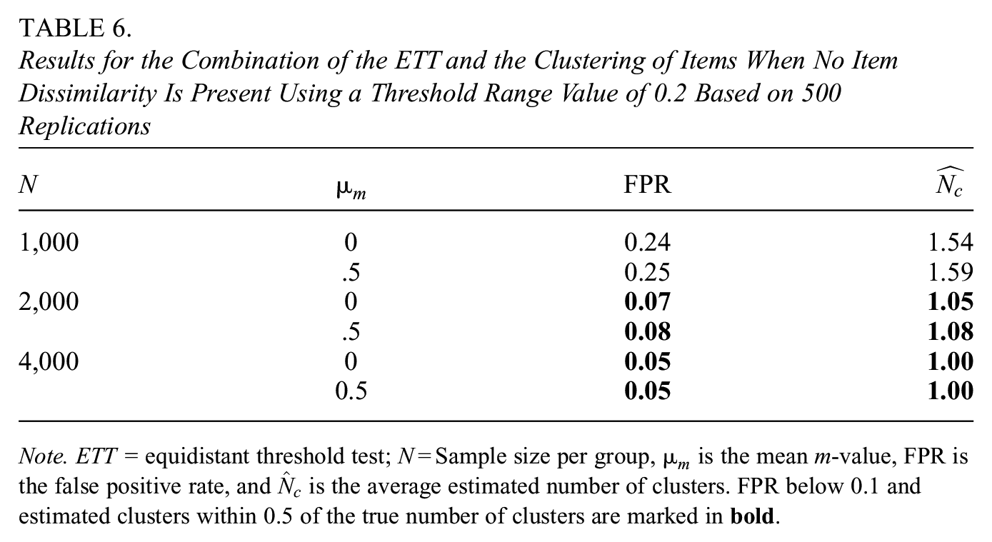Note that an item is labeled as dissimilar if it has either non-equidistant thresholds or if an $E$ -value was added to induce dissimilar functioning. Finally, we included the estimated latent means and variances when the focal cluster is used as the anchoring cluster to ensure no bias results from use of the combined approach. The results for the conditions without DIF can be found in Table 6.

Table 6.

Results for the Combination of the ETT and the Clustering of Items When No Item Dissimilarity Is Present Using a Threshold Range Value of 0.2 Based on 500 Replications

$N$	$μ_{m}$	FPR	$\hat{N_{c}}$
1,000	0	0.24	1.54
	.5	0.25	1.59
2,000	0	0.07	1.05
	.5	0.08	1.08
4,000	0	0.05	1.00
	0.5	0.05	1.00

Note. ETT = equidistant threshold test; N = Sample size per group, $μ_{m}$ is the mean $m$ -value, FPR is the false positive rate, and ${\hat{N}}_{c}$ is the average estimated number of clusters. FPR below 0.1 and estimated clusters within 0.5 of the true number of clusters are marked in bold.

Results for the Combined Approach

Conditions Without DIF

As can be seen in Table 6, the FPR of the approach remains below 0.1 as long as the sample size is at least 2,000 for each group. The FPR can be inflated at lower sample sizes due to the higher standard errors of the $Δ R$ -values potentially leading to the formation of multiple anchor clusters. This effect is greatly diminished by increasing the sample size to 2,000 per group and completely disappears when the sample size is 4,000 per group. Increasing the mean $m$ -value also leads to an increased FPR, likely due to a loss of information leading to higher standard errors for the $Δ R$ values.

Concerning the number of clusters formed, higher sample sizes lead to an $\hat{N_{c}}$ closer to the true number of clusters. Increasing the mean $m$ -value leads to more clusters being formed due to a loss of information, but this effect can be remedied by increasing the sample size. Table 7 displays the results for the conditions with DIF present.

Table 7.

Results for the Combination of the ETT and the Clustering of Items When Item Dissimilarity Is Present Using a Threshold Range Value of 0.2 Based on 500 Replications

$D$	$N$	$μ_{m}$	$E$	$N_{C}$	TPR	FPR	Specificity	$\hat{N_{C}}$	${\hat{μ}}_{2}$	${\hat{σ}}_{1}^{2}$	${\hat{σ}}_{2}^{2}$
0.25	1,000	0	0.25	2	0.90	0.08	0.72	2.24	.00	1.00	1.00
				3	0.90	0.11	0.71	3.16	.00	1.00	1.00
			0.5	2	0.91	0.08	0.74	2.35	.00	1.00	1.00
				3	0.91	0.08	0.75	3.31	.00	1.00	1.00
		.5	0.25	2	0.90	0.09	0.72	2.30	.00	1.00	1.00
				3	0.89	0.12	0.70	3.19	.00	1.00	1.00
			0.5	2	0.91	0.11	0.74	2.51	.01	1.01	.99
				3	0.91	0.09	0.73	3.55	.00	1.01	1.00
	2,000	0	0.25	2	0.97	0.06	0.91	2.01	.00	1.01	1.00
				3	0.97	0.06	0.91	3.00	.00	1.01	1.00
			0.5	2	0.98	0.05	0.92	2.02	.01	1.01	1.00
				3	0.97	0.05	0.92	3.01	.01	1.00	.99
0.5	1,000		0.25	2	0.99	0.07	0.97	2.09	.01	1.01	1.00
				3	0.99	0.10	0.96	3.03	.01	1.01	.99
			0.5	2	1.00	0.07	1.00	2.17	.00	1.00	1.00
				3	1.00	0.08	1.00	3.12	.00	1.00	1.00
	2,000		0.25	2	1.00	0.05	1.00	2.00	.00	1.00	1.00
				3	1.00	0.05	1.00	3.00	.00	1.00	1.00
			0.5	2	1.00	0.05	1.00	2.01	.00	1.00	1.00
				3	1.00	0.04	1.00	3.01	.00	1.00	1.00

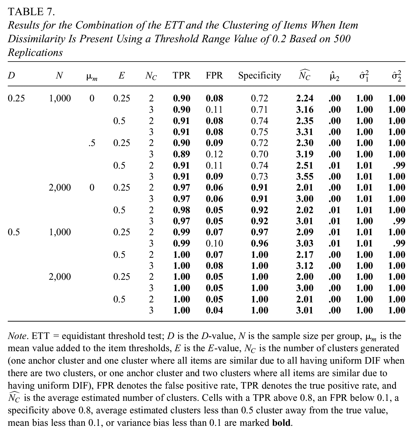
Note. ETT = equidistant threshold test; $D$ is the $D$ -value, N is the sample size per group, $μ_{m}$ is the mean value added to the item thresholds, $E$ is the $E$ -value, $N_{C}$ is the number of clusters generated (one anchor cluster and one cluster where all items are similar due to all having uniform DIF when there are two clusters, or one anchor cluster and two clusters where all items are similar due to having uniform DIF), FPR denotes the false positive rate, TPR denotes the true positive rate, and $\hat{N_{C}}$ is the average estimated number of clusters. Cells with a TPR above 0.8, an FPR below 0.1, a specificity above 0.8, average estimated clusters less than 0.5 cluster away from the true value, mean bias less than 0.1, or variance bias less than 0.1 are marked bold.

Conditions With DIF

As can be seen in Table 7, the TPR is at least 0.9 across all conditions, again showcasing the high TPR of the 0.2 threshold range approach. An underpowered ETT thus does not seem to adversely affect clustering performance. Note that the decrease in TPR from near 1 to 0.9 (and consequent decrease in specificity) is driven by the lower power of the ETT when sample sizes are below 2,000. In essence, we see that the ETT stage of the approach is somewhat more conservative (i.e., retains more items) than the clustering stage. Increasing the sample size or increasing the $D$ -value increases the TPR further. There is no clear effect of changing the $μ_{m}$ value or increasing the $E$ -value. The fact that increasing the $E$ -value does not affect the TPR of the approach again shows that the TPR is mostly determined by the power of the ETT in these conditions.

When considering the FPR, we again see that lower sample sizes can lead to an FPR above 0.1. This is especially the case when multiple DIF clusters are present, and the $E$ -value is low. Increasing the $μ_{m}$ value seems to inflate the FPR somewhat while increasing the $D$ -value has no clear effect on the FPR. Again, the main driver of the FPR seems to be the sample size, with the FPR decreasing greatly if the sample size is increased.

The specificity of the clusters formed mostly seems to be determined by the performance of the ETT. Perhaps not surprisingly, an underpowered ETT leads to a lower specificity of the focal cluster, as items with non-eq8 thresholds are admitted to the focal cluster. The specificity is thus lower for lower sample sizes and lower $D$ -values. The effects of the other factors are minimal. While the lowered specificity and occasionally higher FPR may seem problematic, it may be relevant to emphasize that these effects only occur in the conditions that were handpicked for their poor performance on the ETT.

Regarding the number of estimated clusters, we mostly see a repetition of earlier findings. When $D$ -values, sample sizes, and $E$ -values are higher, the number of clusters formed is closer to the true value of clusters. The true number of clusters and the $μ_{m}$ value do not seem to have much impact in this regard.

Finally, there appears to be little bias in any of the latent trait parameters as long as the focal cluster is used to anchor the scale. This is likely due to the high power of the 0.2 threshold range approach eliminating almost all items with uniform DIF. In addition, the specificity of the focal cluster does stay somewhat high in all conditions, with at least 69% of all items in the cluster being anchor items. It thus seems that as long as most items are anchor items and all uniform DIF items are eliminated, little bias in latent trait parameters occurs.

Discussion

The present study set out to highlight an alternative and empirically identified approach to DIF testing utilizing item (dis)similarity and extended the proposed approaches for dichotomous items to the polytomous case utilizing the PCM. As a first stage in the approach, it is assessed whether items have equidistant thresholds across groups. As the second stage, the items with equidistant thresholds are clustered on all thresholds to reveal clusters of similarly functioning items. The two stages were first evaluated on their individual performance separately and finally on their combined performance. The results will be discussed in this order.

The ETT performed well in most simulated conditions, with the type I error of the approach remaining at the 0.05 level for all conditions. In terms of power, we recommend a sample size of at least 2,000 participants per group if a researcher is interested in detecting the smaller levels of non-equidistant thresholds at a type I error rate of 0.05.

When evaluating the second stage of the approach, a threshold range criterion of 0.2 was considered in the main paper. This approach led to a higher TPR but, in turn, showed a higher FPR than the BIC approach detailed in Supplemental Material A, especially when sample size was below 2,000 participants per group. Researchers aiming to utilize the threshold range approach when the sample sizes per group are below 2,000 could consider increasing the number of items to ensure that after completing this stage, one can expect enough items to remain to construct a valid test. Alternatively, the cluster approach could be combined with traditional DIF testing methods, such as the likelihood-ratio test with the designated DIF-free cluster as an anchor cluster to add more items to the DIF-free cluster.

To assess the performance of the combined approaches, several conditions were considered. First, several conditions where no DIF was present in any item were analyzed. Again, lower sample sizes lead to an inflated FPR when utilizing the 0.2 threshold range approach. It must be noted that the FPR of the combined approach was often somewhat higher than the FPR of the separate approaches. The advice to increase the number of items when dealing with DIF-analysis utilizing a sample size below 1,000 thus holds even stronger for the combined condition. Second, several DIF conditions were considered. In the conditions with DIF present, we were mostly interested in whether an underpowered ETT would adversely affect the performance of the clustering. Fortunately, this did not seem to be the case in the observed conditions. The results of the combined conditions did, however, again emphasize the need for a sample size above 1,000 participants per group or a high number of items to combat the FPR. Notably, no bias in the latent trait occurred in any condition as long as the focal cluster was used as an anchoring cluster.

A final aspect of the approach that must be discussed is how a researcher would designate a cluster as DIF-free in practice. Several approaches to this problem have been proposed previously. First of all, it is possible to designate the cluster with most items as DIF-free (Pohl et al., 2017). Opponents of this approach may call the assumption that most items are DIF-free “wishful thinking” and point to the fact various group-level differences in response style are frequently found (Chun et al., 1974; Clarke, 2001; Marin et al., 1992; Zhang & Wang, 2020). Truly DIF-free items may thus be rare. In addition, it is very well possible the cluster approach results in multiple clusters of the same size.

A second approach to designating the DIF-free cluster is to select the cluster with the lowest variance (Pohl et al., 2017). The logic behind this approach is that the $Δ R$ -values of DIF-free items originate from a distribution with some variance and a constant mean, as all DIF-free items function similarly. On the other hand, the $Δ R$ -values of the DIF items originate from a distribution with some variance and a variable mean, as DIF-free items do not necessarily function similarly. Unless all DIF items function similarly (i.e., have the same extent of uniform DIF), it is thus likely a DIF cluster will have more variance than a DIF-free cluster. One problem with this approach is that it does not account for the existence of single-item clusters, which have a variance of zero and would thus always be preferred.

Finally, one could involve content experts in designating the cluster they believe to be DIF-free. An advantage of this approach is the opportunity to involve substantive expertise in the cluster decision. As a disadvantage, it may prove difficult to isolate the decision process from preexisting biases by the experts and the researcher.

While the proposed approach performs adequately as long as sample sizes are not too small, the current study has limitations, and several avenues for future research remain open. As a first limitation, the current study was a simulation study, where not all conditions may be generalizable to real-life conditions. For example, items were answered with no missing data, the DIF induced in the items was quite uniform in its strength, and only four-category PCM items were examined. Future research should examine the performance of this approach when conditions such as these are varied.

Second, the approach should be extended to different IRT models. Note that while the approach presented here was illustrated using four-category items, extensions to items with more categories can be achieved by simply increasing the number of distances tested in the ETT. While several operationalizations of these distances are possible, it may be simplest to conceive of the distances as the space between two neighboring thresholds. In addition, the approach described here could be generalized to the GPCM by starting with an additional clustering step on the log slopes as described in Pohl et al. (2021) and implementing the approach described in this paper conditional on items being in the same slope cluster. While the extension of the approach described here to the GPCM may be theoretically straightforward, several practical questions remain. First of all, it is not yet clear how clustering on slopes rather than thresholds will influence the sample size required for the method to function adequately. Second, increasing the number of clustering stages, as proposed by Pohl et al. (2021), may adversely affect the FP rate of the approach. Further research is needed in these areas. In addition to the GPCM, the approach could be extended in a similar way to the graded response model (Samejima, 1969). Again, further research is needed when evaluating the efficacy of the approach for this model.

As a third limitation, it is not yet clear which method of clustering items will perform best under which conditions. While the current paper considered k-means clustering on an arbitrary row of the $Δ R$ matrix, other approaches may be considered. For example, hierarchical clustering based on the absolute values of the entire $Δ R$ matrix could be considered. If a researcher additionally wants to take the uncertainty of the variables into account, one could even consider constructing the Wald statistics of the $Δ R$ matrix, as Bechger and Maris (2015) propose, and hierarchically cluster these values. Future research should evaluate the efficacy of various clustering approaches in different conditions. In addition, other approaches to determining the number of clusters should be considered. For example, an adaptive threshold range approach where the value of the threshold range is dependent on the (average) standard error of the $Δ R$ -values could be considered.

Fourth, the current paper proposes a Wald test when establishing whether items have equidistant thresholds or not. While the approach performs reasonably in the simulated conditions, other approaches, such as bootstrap tests or Bayesian methods, are possible and may show superior performance. Alternative approaches to the first step may also relax the assumption of completely equidistant thresholds across items, for example, in favor of approximately equidistant thresholds. Future research should evaluate the performance of these approaches.

Fifth, the current paper limits its scope to situations where only two clearly defined groups are present. Future research would do well to extend the method to situations where groups are not clearly defined (e.g., latent classes are present in the data). Additionally, scenarios with more than two groups present should be examined. When many groups are present, one may consider mixture-multigroup factor analysis methods to reduce inflated type I error rates resulting from many pairwise comparisons (De Roover, 2021; De Roover et al., 2022).

Finally, the current paper aims to detect items that are fully measurement invariant. To identify the model, technically, only a single threshold of a single item needs to be set to be equivalent across groups. While it is naturally preferred for items to achieve full rather than partial invariance, future research could examine the performance of the approach if some aspects of the invariance were relaxed.

From this paper, several practical recommendations can be made. First of all, researchers should consider their conceptualization of DIF. As DIF is not empirically identifiable, they may wish to think in terms of similar/dissimilar item functioning instead. This approach to DIF has several conceptual advantages, such as being rooted in empiricism and forcing researchers to explicate their assumptions about DIF when designating a DIF-free cluster.

Second, researchers should assess what their beliefs about DIF are when designating a DIF-free cluster. A central point of contention here will be if the assumption that most items are DIF-free is realistic or not. We encourage researchers to explicate their beliefs and allow other researchers to see what results would have been if different assumptions were made, which is most easily achieved by utilizing the cluster-based approach to DIF.

Third, researchers should consider what the maximum amount of DIF they are willing to accept is. Formulating what amount of DIF is “acceptable” will aid in choosing an appropriate threshold range criterion. If the amount of DIF one accepts is too great, many items will erroneously be placed in the same cluster (this can be seen when examining the results for the 0.4 and 0.6 threshold ranges in Supplemental Material A). If the amount of DIF one accepts is too small, many items will be wrongly placed in different clusters. To inform the size of the threshold, one may refer to benchmarks of DIF in large-scale assessments, as suggested by Pohl et al. (2021). Alternatively, one could consider the standard errors of the $Δ R$ values to inform their decision, with smaller standard errors leading to smaller threshold ranges and vice versa. If the maximum amount of DIF a researcher is willing to accept is small, sample size considerations should also be made to avoid a high FPR when applying the cluster-based approach described in this paper.

Summarizing, the current paper extends the cluster approach to DIF to polytomous items. We advocate for a two-stage approach, where the distances between thresholds within an item across groups are compared first. Second, items that are found to have equidistant thresholds are clustered on all thresholds. The proposed approach can bring many conceptual and practical advantages to the DIF testing framework, and we encourage researchers to consider their conceptualization of and assumptions about DIF.

Supplemental Material

sj-docx-1-jeb-10.3102_10769986241256033 – Supplemental material for Extending the Cluster Approach to Differential Item Functioning in Polytomous Items

Supplemental material, sj-docx-1-jeb-10.3102_10769986241256033 for Extending the Cluster Approach to Differential Item Functioning in Polytomous Items by Martijn Schoenmakers, Jesper Tijmstra, Jeroen Vermunt and Maria Bolsinova in Journal of Educational and Behavioral Statistics

Supplemental Material

sj-zip-2-jeb-10.3102_10769986241256033 – Supplemental material for Extending the Cluster Approach to Differential Item Functioning in Polytomous Items

Supplemental material, sj-zip-2-jeb-10.3102_10769986241256033 for Extending the Cluster Approach to Differential Item Functioning in Polytomous Items by Martijn Schoenmakers, Jesper Tijmstra, Jeroen Vermunt and Maria Bolsinova in Journal of Educational and Behavioral Statistics

Footnotes

Declaration of Conflicting Interests

The author(s) declared no potential conflicts of interest with respect to the research, authorship, and/or publication of this article.

Funding

The author(s) received no financial support for the research, authorship, and/or publication of this article.

ORCID iD

Martijn Schoenmakers

Notes

Authors

MARTIJN SCHOENMAKERS is a PhD candidate at the Department of Methodology and Statistics, Tilburg School of Social and Behavioral Sciences, Tilburg University, PO Box 90513, 5000LE, Tilburg, The Netherlands, e-mail: m.schoenmakers@tilburguniversity.edu. His main research interests are item response theory, response styles, and differential item functioning.

JESPER TIJMSTRA is an assistant professor at the Department of Methodology and Statistics, Tilburg School of Social and Behavioral Sciences, Tilburg University, PO Box 90513, 5000LE, Tilburg, The Netherlands, e-mail: j.tijmstra@tilburguniversity.edu. His research focuses on psychometrics, with an emphasis on item response theory.

JEROEN VERMUNT is a full professor at the Department of Methodology and Statistics, Tilburg School of Social and Behavioral Sciences, Tilburg University, PO Box 90153, 5000LE, Tilburg, The Netherlands, e-mail: j.k.vermunt@tilburguniversity.edu. His research interests include latent class and finite mixture models, IRT modeling, longitudinal and event history data analysis, multilevel analysis, and generalized latent variable modeling.

MARIA BOLSINOVA is an assistant professor at the Department of Methodology and Statistics, Tilburg School of Social and Behavioral Sciences, Tilburg University, PO Box 90513, 5000LE, Tilburg, The Netherlands, e-mail: m.a.bolsinova@tilburguniversity.edu. Her main research interests are item response theory, process data, and adaptive learning.

References

Bechger

T. M.

Maris

(2015). A statistical test for differential item pair functioning. Psychometrika, 80(2), 317–340. https://doi.org/10.1007/s11336-014-9408-y

Byrne

B. M.

Watkins

(2003). The issue of measurement invariance revisited. Journal of Cross-Cultural Psychology, 34(2), 155–175. https://doi.org/10.1177/0022022102250225

Chalmers

R. P.

(2012). mirt: A Multidimensional item response theory package for the R environment. Journal of Statistical Software, 48, 1–29. https://doi.org/10.18637/jss.v048.i06

Chun

K.-T.

Campbell

J. B.

Yoo

J. H.

(1974). Extreme response style in cross-cultural research: A reminder. Journal of Cross-Cultural Psychology, 5(4), 465–480. https://doi.org/10.1177/002202217400500407

Clarke

(2001). Extreme response style in cross-cultural research. International Marketing Review, 18(3), 301–324. https://doi.org/10.1108/02651330110396488

Cohen

A. S.

Kim

S.-H.

Wollack

J. A.

(1996). An investigation of the likelihood ratio test for detection of differential item functioning. Applied Psychological Measurement, 20(1), 15–26. https://doi.org/10.1177/014662169602000102

De Roover

(2021). Finding clusters of groups with measurement invariance: Unraveling intercept non-invariance with mixture multigroup factor analysis. Structural Equation Modeling: A Multidisciplinary Journal, 28(5), 663–683. https://doi.org/10.1080/10705511.2020.1866577

De Roover

Vermunt

J. K.

Ceulemans

(2022). Mixture multigroup factor analysis for unraveling factor loading noninvariance across many groups. Psychological Methods, 27(3), 281–306. https://doi.org/10.1037/met0000355

Jin

K.-Y.

Wang

W.-C.

(2014). Generalized IRT models for extreme response style. Educational and Psychological Measurement, 74(1), 116–138. https://doi.org/10.1177/0013164413498876

10.

Jodoin

M. G.

Gierl

M. J.

(2001). Evaluating Type I error and power rates using an effect size measure with the logistic regression procedure for DIF detection. Applied Measurement in Education, 14(4), 329–349. https://doi.org/10.1207/S15324818AME1404_2

11.

Kim

S.-H.

Cohen

A. S.

(1991). A comparison of two area measures for detecting differential item functioning. Applied Psychological Measurement, 15(3), 269–278. https://doi.org/10.1177/014662169101500307

12.

Kim

S.-H.

Cohen

A. S.

(1995). A comparison of lord’s chi-square, Raju’s area measures, and the likelihood ratio test on detection of differential item functioning. Applied Measurement in Education, 8(4), 291–312. https://doi.org/10.1207/s15324818ame0804_2

13.

Kim

S.-H.

Cohen

A. S.

(1998). Detection of differential item functioning under the graded response model with the likelihood ratio test. Applied Psychological Measurement, 22(4), 345–355. https://doi.org/10.1177/014662169802200403

14.

Kopf

Zeileis

Strobl

(2015a). A framework for anchor methods and an iterative forward approach for DIF Detection. Applied Psychological Measurement, 39(2), 83–103. https://doi.org/10.1177/0146621614544195

15.

Kopf

Zeileis

Strobl

(2015b). Anchor selection strategies for DIF analysis. Educational and Psychological Measurement, 75(1), 22–56. https://doi.org/10.1177/0013164414529792

16.

Lord

F. M.

(1980). Applications of item response theory to practical testing problems. Routledge. https://doi.org/10.4324/9780203056615

17.

Marin

Gamba

R. J.

Marin

B. V.

(1992). Extreme response style and acquiescence among hispanics: The role of acculturation and education. Journal of Cross-Cultural Psychology, 23(4), 498–509. https://doi.org/10.1177/0022022192234006

18.

Masters

G. N.

(1982). A rasch model for partial credit scoring. Psychometrika, 47(2), 149–174. https://doi.org/10.1007/BF02296272

19.

Millsap

R. E.

Everson

H. T.

(1993). Methodology review: Statistical approaches for assessing measurement bias. Applied Psychological Measurement, 17(4), 297–334. https://doi.org/10.1177/014662169301700401

20.

OECD. (2000). Measuring student knowledge and skills: The PISA 2000 assessment of reading, mathematical and scientific literacy.

21.

OECD. (2010). PISA 2009 Assessment framework: Key competencies in reading, mathematics and science. https://www.oecd-ilibrary.org/education/pisa-2009-assessment-framework_9789264062658-en

22.

Penfield

R. D.

Camilli

(2006). 5 Differential item functioning and item bias. In Rao

C. R.

Sinharay

(Eds.), Handbook of statistics (Vol. 26, pp. 125–167). Elsevier. https://doi.org/10.1016/S0169-7161(06)26005-X

23.

Pohl

Schulze

(2020). Assessing group comparisons or change over time under measurement non-invariance: The cluster approach for nonuniform DIF. Psychological Test and Assessment Modeling, 62(2), 281–303.

24.

Pohl

Schulze

Stets

(2021). Partial measurement invariance: Extending and evaluating the cluster approach for identifying anchor items. Applied Psychological Measurement, 45(7–8), 477–493. https://doi.org/10.1177/01466216211042809

25.

Pohl

Stets

Carstensen

C. H.

(2017). Cluster-based Anchor Item Identiﬁcation and Selection (NEPS Working Paper No. 68). Leibniz Institute for Educational Trajectories, National Educational Panel Study.

26.

Pustejovsky

J. E.

(2023, July 19). Wald tests of multiple-constraint null hypotheses. https://cran.r-project.org/web/packages/clubSandwich/vignettes/Wald-tests-in-clubSandwich.html

27.

R Core Team. (2022). R: A language and environment for statistical computing. R Foundation for Statistical Computing, Vienna, Austria.

28.

Samejima

(1969). Estimation of latent ability using a response pattern of graded scores. Psychometrika Monograph Supplement, 34(4, Pt. 2), 100. https://psycnet.apa.org/record/1972-04809-001

29.

Van

Schoot

Schmidt

De Beuckelaer

Lek

Zondervan-Zwijnenburg

(2015). Editorial: Measurement invariance. Frontiers in Psychology, 6. https://www.frontiersin.org/articles/10.3389/fpsyg.2015.01064

30.

Wang

Song

(2011). Ckmeans.1d.dp: Optimal k-means clustering in one dimension by dynamic programming. The R Journal, 3(2), 29. https://doi.org/10.32614/RJ-2011-015

31.

Wang

W.-C.

Yeh

Y.-L.

(2003). Effects of anchor item methods on differential item functioning detection with the likelihood ratio test. Applied Psychological Measurement, 27(6), 479–498. https://doi.org/10.1177/0146621603259902

32.

Woods

C. M.

(2009). Empirical selection of anchors for tests of differential item functioning. Applied Psychological Measurement, 33(1), 42–57. https://doi.org/10.1177/0146621607314044

33.

Zhang

Wang

(2020). Validity of three IRT models for measuring and controlling extreme and midpoint response styles. Frontiers in Psychology, 11, 271. https://doi.org/10.3389/fpsyg.2020.00271

Supplementary Material

Please find the following supplemental material available below.

For Open Access articles published under a Creative Commons License, all supplemental material carries the same license as the article it is associated with.

For non-Open Access articles published, all supplemental material carries a non-exclusive license, and permission requests for re-use of supplemental material or any part of supplemental material shall be sent directly to the copyright owner as specified in the copyright notice associated with the article.

0.00 MB

0.07 MB

0.02 MB