
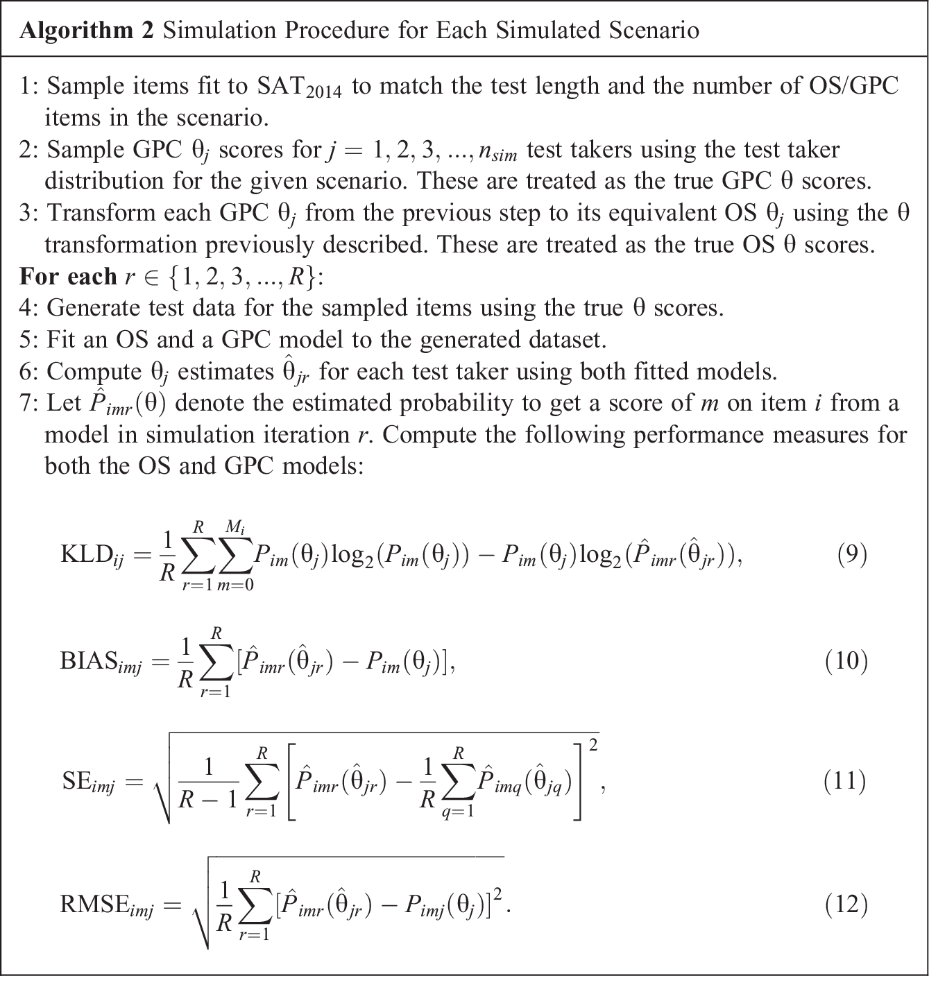
Abstract
Item response theory (IRT) models the relationship between the possible scores on a test item against a test taker’s attainment of the latent trait that the item is intended to measure. In this study, we compare two models for tests with polytomously scored items: the optimal scoring (OS) model, a nonparametric IRT model based on the principles of information theory, and the generalized partial credit (GPC) model, a widely used parametric alternative. We evaluate these models using both simulated and real test data. In the real data examples, the OS model demonstrates superior model fit compared to the GPC model across all analyzed datasets. In our simulation study, the OS model outperforms the GPC model in terms of bias, but at the cost of larger standard errors for the probabilities along the estimated item response functions. Furthermore, we illustrate how surprisal arc length, an IRT scale invariant measure of ability with metric properties, can be used to put scores from vastly different types of IRT models on a common scale. We also demonstrate how arc length can be a viable alternative to sum scores for scoring test takers.
1. Introduction
Most performance tests are scored by adding up predetermined item scores. We will refer to scores resulting from this method as sum scores. Let
Some examples of large-scale tests using sum scores include the Scholastic Aptitude Test (SAT) or tests produced by the American College Testing program (Dorans, 1999). A downside of sum scores is that all items contribute equally to the overall score and implicitly to the underlying trait the test aims to measure. This is typically not the case, and a good alternative to using sum scores is to score test takers with item response theory (IRT). IRT scores take properties of each individual item into account, and different items have different levels of precision for different trait levels. For instance, a hard item might better discriminate among individuals with high ability levels but would be less informative for individuals with low abilities. Consequently, IRT can more precisely estimate an individual’s trait level across the entire trait spectrum and also allows for uncertainty estimates of the scores to differ across the score scale. As a consequence, IRT scores are also less affected by items measuring something different than intended.
Additionally, IRT models are commonly used to solve a wide range of practical test related problems. Examples include test equating, establishing the psychometric properties of test forms and test items as well as optimizing the efficiency of test delivery in more complex assessment systems. Parametric IRT models (Lord, 1980) have been the most common choice in the past. A disadvantage with parametric IRT is that, even in well-designed tests, some items may not fit a parametric IRT model. When this is the case, using a nonparametric IRT model can be preferable.
For binary scored items, several nonparametric estimation methods have been suggested. Mokken (1997) studied monotonicity and nonparametric estimation for binary scored items. Ramsay (1991, 1997) proposed to estimate item response functions (IRFs) with kernel smoothing over quantiles of the Gaussian distribution. Rossi et al. (2002) and Ramsay and Silverman (2002) optimized the penalized marginal likelihood using the expectation–maximization algorithm, and their IRFs were close to the three parameter logistic IRT model when the roughness penalty increased. Ramsay and Silverman (2005) also proposed a nonparametric method for not strictly monotonic curve estimates. Woods and Thissen (2006) and Woods (2006) used a spline-based approximation of the ability distribution when estimating the item parameters. Lee (2007) compared several methods for nonparametric estimation of item characteristic curves for binary items.
Items with more than two scored outcomes are commonly referred to as polytomously scored items. Such items are used in a variety of settings, including the scoring of rated tasks, the scoring of testlets or groups of dependent dichotomously scored items, multiple-choice items for which the incorrect options are retained for scoring purposes, and rating scales used to measure psychological and behavioral traits. Nonparametric IRT for polytomously scored items was first proposed by Molenaar (1997), after which a wide variety of nonparametric/semiparametric approaches have been studied (Emons, 2008; Falk & Cai, 2016; Sijtsma & Molenaar, 2002; Stochl et al., 2012). Emons (2008) examined the effectiveness of generalizations of nonparametric person-fit statistics to polytomous item response data. Stochl et al. (2012) examined Mokken scale polytomous rating scale health data coded as 1–2–3–4 and recoded them as 0–0–1–1, thus essentially making the items binary before analyzing the data. Falk and Cai (2016) compared the monotonic polynomial method to other nonparametric and semiparametric alternatives. More recently, Ramsay et al. (2020) studied the nonparametric optimal scoring (OS) approach for rating scale data.
The OS IRT framework introduces new interesting perspectives to IRT. Through the fusion of psychometric and information theory, the arc length
Prior research on OS has mostly focues on binary scored multiple choice items (Ramsay & Wiberg, 2017). Ramsay et al. (2019) notably expanded the scope by taking the information from all incorrectly chosen response alternatives into account. A comparison of binary scored items using parametric and nonparametric IRT revealed that sum-scored tests would need to be longer than an optimally scored test in order to attain the same level of accuracy (Wiberg et al., 2019). OS also offers a flexible alternative for estimating IRFs of items that do not show a good fit with parametric IRT models (Ramsay et al., 2019). Recently, OS was proposed as an alternative for analyzing rating scales, which are commonly found in health instruments and questionnaires (Ramsay et al., 2020). Although OS for rating scales was explored in Ramsay et al. (2020), OS for polytomous response data has not yet been compared with parametric IRT.
The overall aim of this study is to compare OS with parametric IRT for polytomously scored items and sum scores, using both simulated and real data. Specifically, we evaluate and compare the item fit and performance of OS against the generalized partial credit (GPC) model, a commonly used parametric IRT model for polytomous response data where test takers can receive partial credit on an item. Additionally, IRT estimated test taker scores, transformed to a ratio scale using the previously mentioned arc length
In Sections 2 and 3, the GPC and OS models are described. After that, the concept of arc length is introduced in Section 4 as an IRT ability scale invariant measure of ability to compare scores from different types of IRT models. The OS and GPC models are then used to analyze real test data in Section 5, followed by a simulation study to make comparison between the two approaches in Section 6. Finally, the paper ends with a discussion with concluding remarks, advantages, disadvantages, and practical implications in Section 7.
2. The GPC Model
The GPC model (Muraki, 1992) is an extension of the partial credit model (Masters, 1982). It can be used to model polytomously scored items, where the items can yield partial credit based on the respondent’s degree of attainment with the underlying trait. The GPC model, similar to most parametric IRT models, requires that the probability of each score on each test item varies smoothly over an index
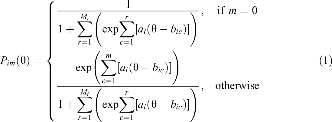
where ai
is the item discrimination parameter and
Unidimensionality: Test taker ability
Local independence: Item responses are conditionally independent given
Monotonicity: The probability of obtaining a score of m or higher is monotonically increasing in
3. Optimal Scoring
The first proposal of OS for binary scored items was made by Ramsay and Wiberg (2017), and they showed that OS can be beneficial in comparison to sum scores. In a later proposal, Ramsay et al. (2019) incorporated information of the incorrect response alternatives as this information proved to give valuable information. Recently, Ramsay et al. (2020) demonstrated the use of OS for polytomous-ordered response scales with clinical data.
In parametric IRT,
3.1. Surprisal and Probability
Surprisal, which originates from information theory (Shannon, 1948), is a central concept within the OS framework. A probability P can be transformed into surprisal using the transformation
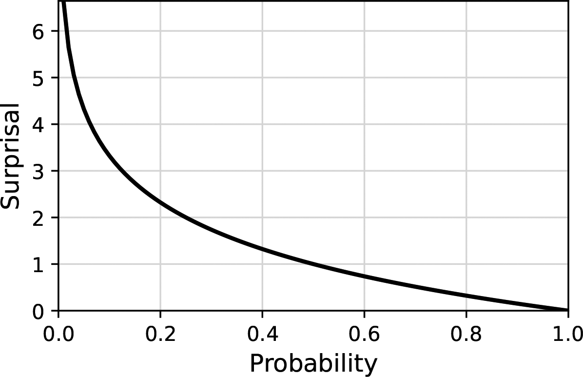
Probability plotted against the corresponding surprisal (2-bit).
The unit of measurement for surprisal depends on the base of the logarithm used in the computation: If base 2 is used, the unit is “bit”; if base 3 is used, the unit is “trit”; and if base 10 is used, the unit is “Hartley” or “dit.” In this article, when we mention “M-bit,” we are referring to the unit of measurement for surprisal based on the logarithm with base M. This concept of “bits” (2-bits) comes from the realm of digital computing, where “bit” is short for “binary digit,” the smallest increment of data on a machine. A bit can hold only one of two values: 0 or 1. Similarly, in information theory, a bit of information represents a decision between two equally likely alternatives.
For example, the probability of landing 3 heads in a row when flipping a coin is
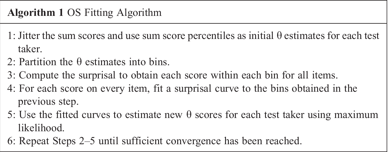
3.2. OS Algorithm
OS models are estimated using an iterative estimation algorithm. The algorithm alternates between using splines to model the surprisal for each score against
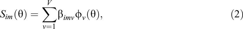
where
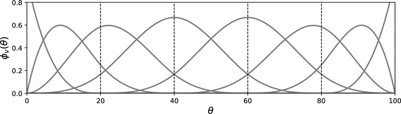
B-spline basis functions
For more information about splines and how to estimate curves refer to Ramsay and Silverman (2005) and Ramsay et al. (2009). To assure that the surprisal corresponding probabilities within each item sum to one for all
is proportional to surprisal. The MLE of
Note that only the chosen response options with associated surprisal curve derivatives contribute to the summations. The assumptions of unidimensionality and local independence required for the GPC model persist for the OS model, as the spline curves are fit independently of each other conditional on
4. Arc Length as a Measure of Ability
A direct comparison of OS estimated
The concept of arc length gives us a solution to the ability comparison problem. The surprisal curves from each item category obtained from a fitted IRT model together define a smooth one-dimensional curve in multidimensional space, parameterized by
Since surprisal is measured in bits,
One should also note Equation 5 is a one-to-one monotonic transformation function of
Furthermore, arc length operates on a ratio scale, possessing an absolute zero. As opposed to using a
Arc length has been used in previous research on OS (e.g., Ramsay et al., 2023; Ramsay et al., 2020) and is also implemented in the
There is also a fundamental difference between OS and parametric IRT. For the parametric models such as the GPC model, the
Because of the above, we calculate arc length for the GPC model by setting
5. Empirical Study
Parametric and OS IRT models were fit to four real data sets from two different tests: two data sets from the Swedish SAT, one from 2013 (
Summary Statistics for Each Test Form
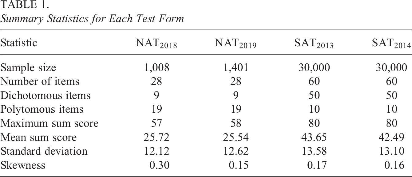
5.1. Swedish National Mathematics Test
The national mathematics test is given to high-school students in Sweden taking the mathematics 3c course. The course is mandatory for students taking the natural science and technology programs but can also be taken by students from other programs by choice. The test is distributed by the end of the course and has a big impact on the course grade. It contains a mix of different item types, some being dichotomously scored while others are scored polytomously.
5.2. Verbal Swedish SAT
The Swedish SAT is administered twice a year and is used when applying for higher education in Sweden. It consists of a verbal and a quantitative part. Only the verbal part was considered in this study. The verbal part contains multiple-choice items of three different types: word interpretation, sentence completion, and reading comprehension. In the third type, texts are presented to the test taker and several multiple-choice items relate to each text. Responses to items relating to the same text cannot be assumed independent given a certain level of a unidimensional underlying trait, as different test takers may be more or less familiar with the text subject. Because of this, scores from items related to the same text were added together and treated as polytomous.
5.3. Fitting Procedure and Evaluation Metrics
GPC models were fitted to
To evaluate model fit while still adjusting for overfitting, 10-fold cross validation (CV) was used to estimate the out-of-sample LL for each model. Specifically, each data set was subset into 10 equally sized folds

where nf
is the number of test takers in fold f.
Additionally, a comparison method based on binning the data over the

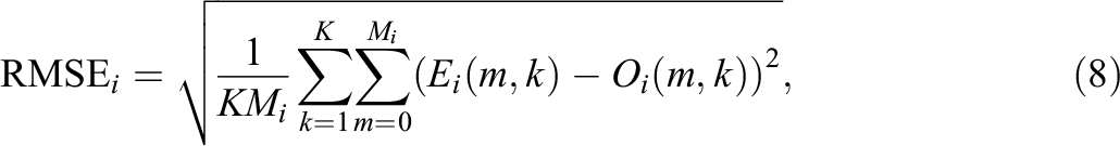
where
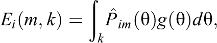
where
5.4. Comparing IRFs
The GPC model was compared against OS models fitted to the same data set using different settings for bins, knots, and spline orders. KLD, RMSE, and CV LL for a large set of fitted models using the different combinations of OS parameter values are provided in Tables A1 to A4 in Online Appendix A. These combinations were chosen to cover a large range of settings, and it is clear from the results that further increasing the flexibility results in overfitting.
Table 2 shows the performance measures for a selected subset of models, which performed relatively well. KLD and RMSE were averaged over all bins, items, and item scores for a fitted model. If a model performed well using one evaluation bin size, it generally performed better throughout the other evaluation bin sizes. The CV LL was smaller for less flexible models fit to the Swedish SAT data, and models using order 4 splines without knots fit to 5 bins performed the best. For the national mathematics data sets, CV LL sometimes favored more flexible OS models despite the much smaller samples. Using 20 bins with no knots was the best setting for both data sets in terms of this metric, with order 5 and order 4 splines for
Performance Measures for Fitted IRT Models
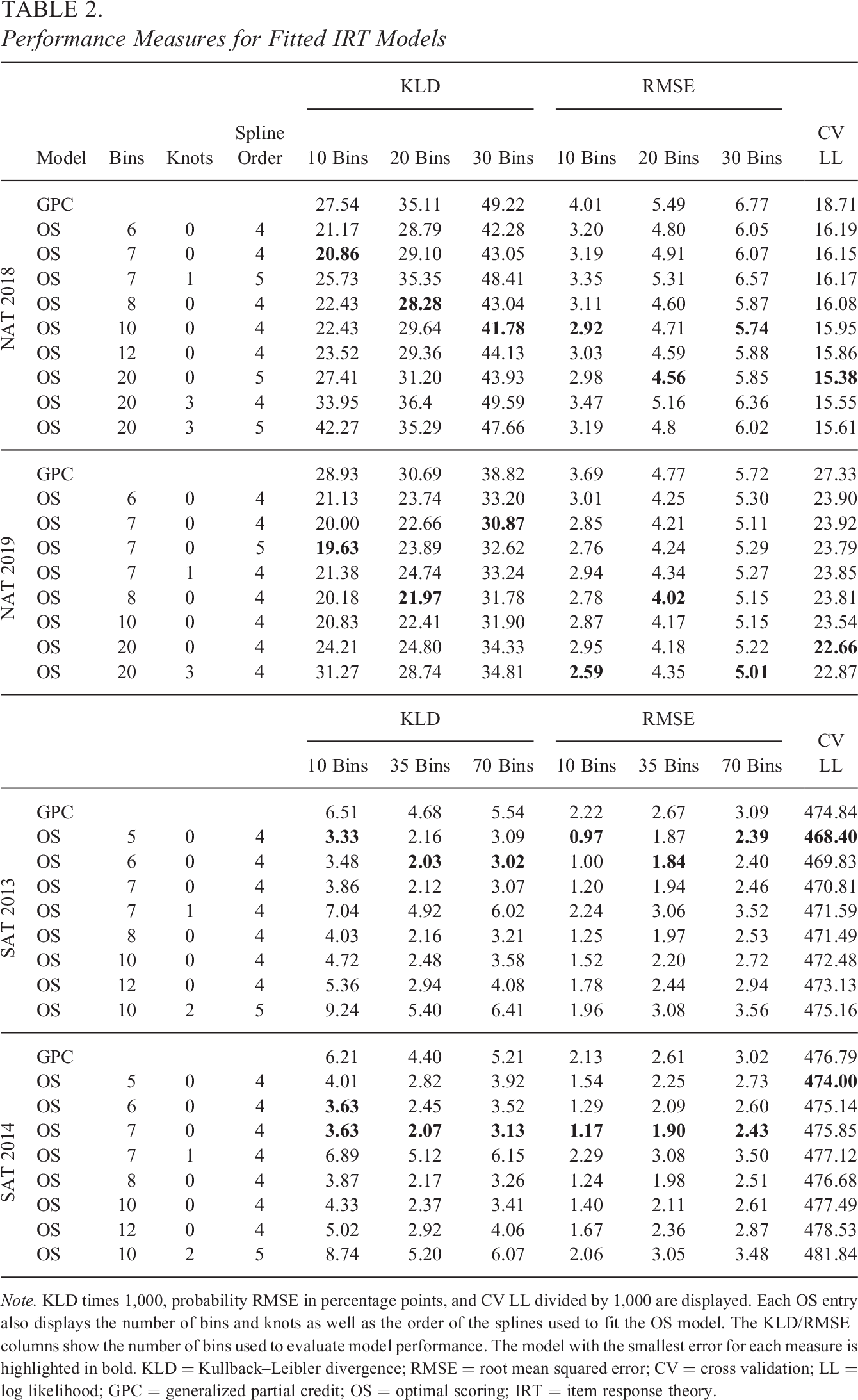
Note. KLD times 1,000, probability RMSE in percentage points, and CV LL divided by 1,000 are displayed. Each OS entry also displays the number of bins and knots as well as the order of the splines used to fit the OS model. The KLD/RMSE columns show the number of bins used to evaluate model performance. The model with the smallest error for each measure is highlighted in bold. KLD = Kullback–Leibler divergence; RMSE = root mean squared error; CV = cross validation; LL = log likelihood; GPC = generalized partial credit; OS = optimal scoring; IRT = item response theory.
In terms of KLD and RMSE, simpler OS models generally outperformed more flexible ones, using higher spline orders and/or multiple knots, for all data sets. However, there were some exceptions to this, especially for the Swedish national mathematics tests. For example, the OS model fit using 20 bins, three knots, and order 4 splines outperformed the GPC model on
For all data sets, better fitting OS models could be identified for all evaluation metrics, but there were also OS parameter combinations, which would result in worse performance for OS.
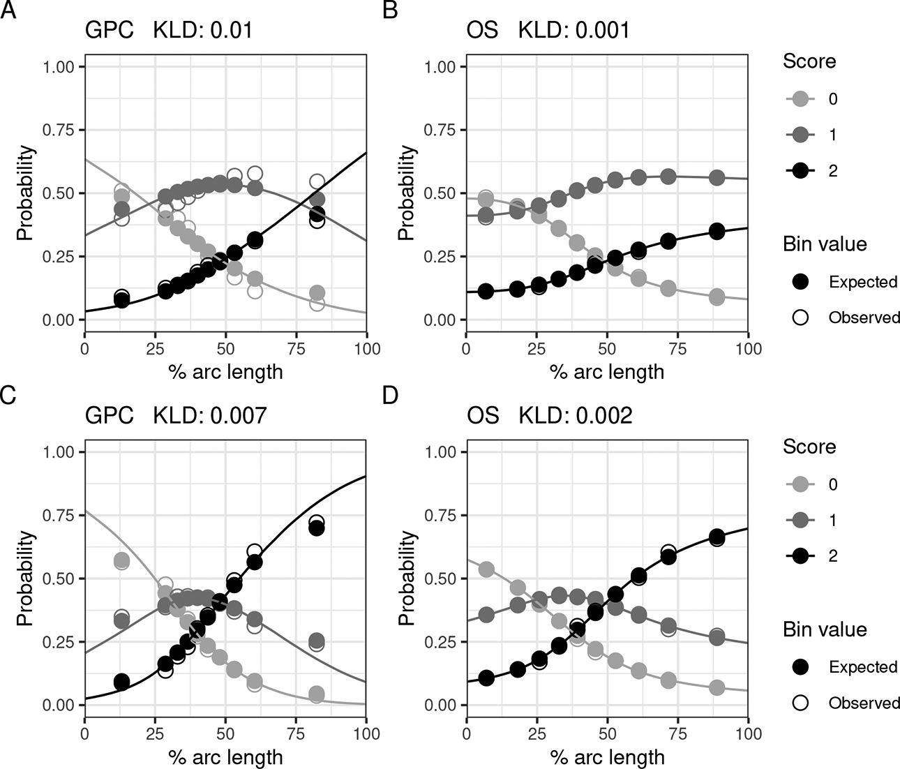
Figures 3 and 4 show IRFs for some of the worst fitting polytomously scored items on
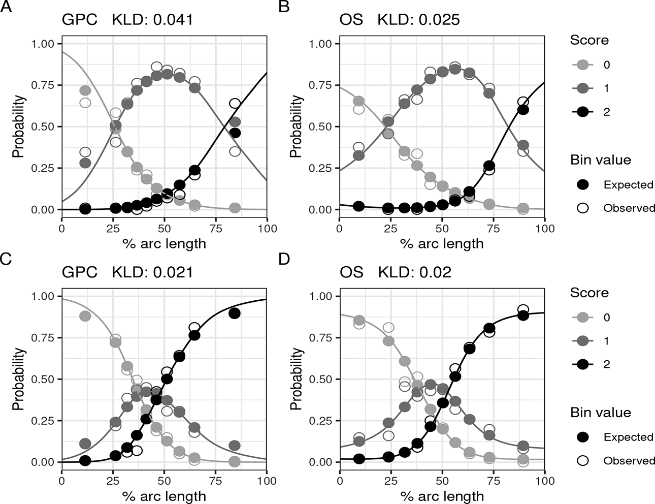
Various item response functions from
Various item response functions from
Plots A and B in Figure 3 show the GPC and OS IRFs from the item with the worst RMSE performance using the GPC model. For this item, the parametric form of the GPC model struggles to model the probabilities for top performing test takers, plot A. The GPC model suggests that the expected probability for a test taker among the top 10% to get the max score on the item is lower than the expected probability to get the second highest score. However, for the observed probabilities in the data, the reverse is true, as shown by the nonfilled dots. When using the best-performing OS model, plot B, the expected probabilities for the top 10% align more closely to the observed ones when compared to the GPC model, plot A.
Plot D in 3 shows the IRF for the item with the worst fit for the OS model, while plot C shows the IRFs for the same item for the GPC model. Even though it has the largest KLD out of all polytomously scored items for the OS model, the KLD is still marginally smaller than the resulting KLD from the GPC model for the same item. Despite this, there are some bins for which the GPC model has a better fit.
IRFs from the worst fitting polytomously scored items on
Plots similar to those in Figures 3 and 4 for
5.5. Score Comparison
Figure 5 shows the kernel-smoothed score distributions for sum scores and percentage arc length
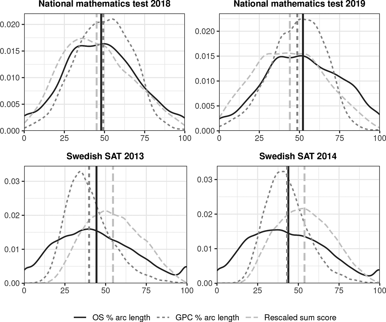
Estimated score distributions resulting from different scoring methods. Each vertical line shows the mean for the corresponding distribution.
Despite
So which score is better? In all four plots in Figure 5, a larger portion of test takers end up closer to or at the score scale boundaries when using OS compared to the other scoring methods. This makes perfect sense for the Swedish SATs, which only contain multiple-choice items. A person not knowing the answer to a single question would be guessing, still accommodating an average of 20% correct responses as all items in the Swedish SATs have five response options each. This is also under the assumption that all distractor options are equally plausible to the true one, which is very hard to achieve. In this sense, the sum score is by definition a biased score estimate for these types of tests if the score is meant to represent a test taker’s attained knowledge of the information contained within the test.
Moreover, even for a well constructed test such as the Swedish SAT, it is inevitable that some items will perform better or worse, both in general and for different test takers. Examples of worse performing items include items with confusing distractor options, unclear problem descriptions, or items that are less related to the underlying construct(s) the test is meant to measure. Since the Swedish SAT is used for applying to university, such items can be punishing, as all items have the same impact on the resulting sum scores. In this respect, the sum score is a worse choice than
For the national mathematics tests, the score distributions of each scoring method are more similar. The items on these tests are not multiple-choice questions, and it is not as clear just from context which distribution is more reasonable/desirable. The ordering of the test takers from using each scoring method is also very similar, with Spearman correlations ranging between 0.978 and 0.997 for all score pairs on all four tests. However, the inherent benefits from IRT of more accurate weighting of items with various relationships with the underlying latent trait together the theoretical concept of a ratio scale from an information theory perspective should speak in the favor of the % arc length scores.
6. Simulation Study
To further compare the fit of parametric IRT and OS IRT models, a simulations study was conducted. Data were generated using IRFs from models fit to the
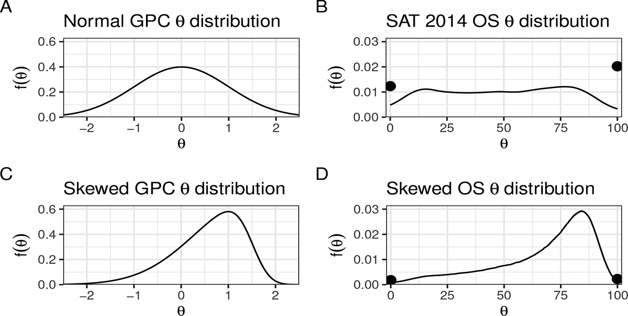
Ability density functions used to generate test data in the simulation study. The dots in the OS distribution plots mark the proportions of test takers at the min/max values of
To be able to generate item scores for test takers using a mixture of OS and GPC IRFs, each test taker’s GPC
The methods were compared throughout various realistic scenarios. The sample size was either 1,000, 5,000, or 10,000 test takers and test lengths of 30 and 60 items were examined. Furthermore, the percentage of OS IRFs used for data generation was varied between 0%,
IRF probability estimation was evaluated over
6.1. Simulation Study Results
Simulation Performance Measures
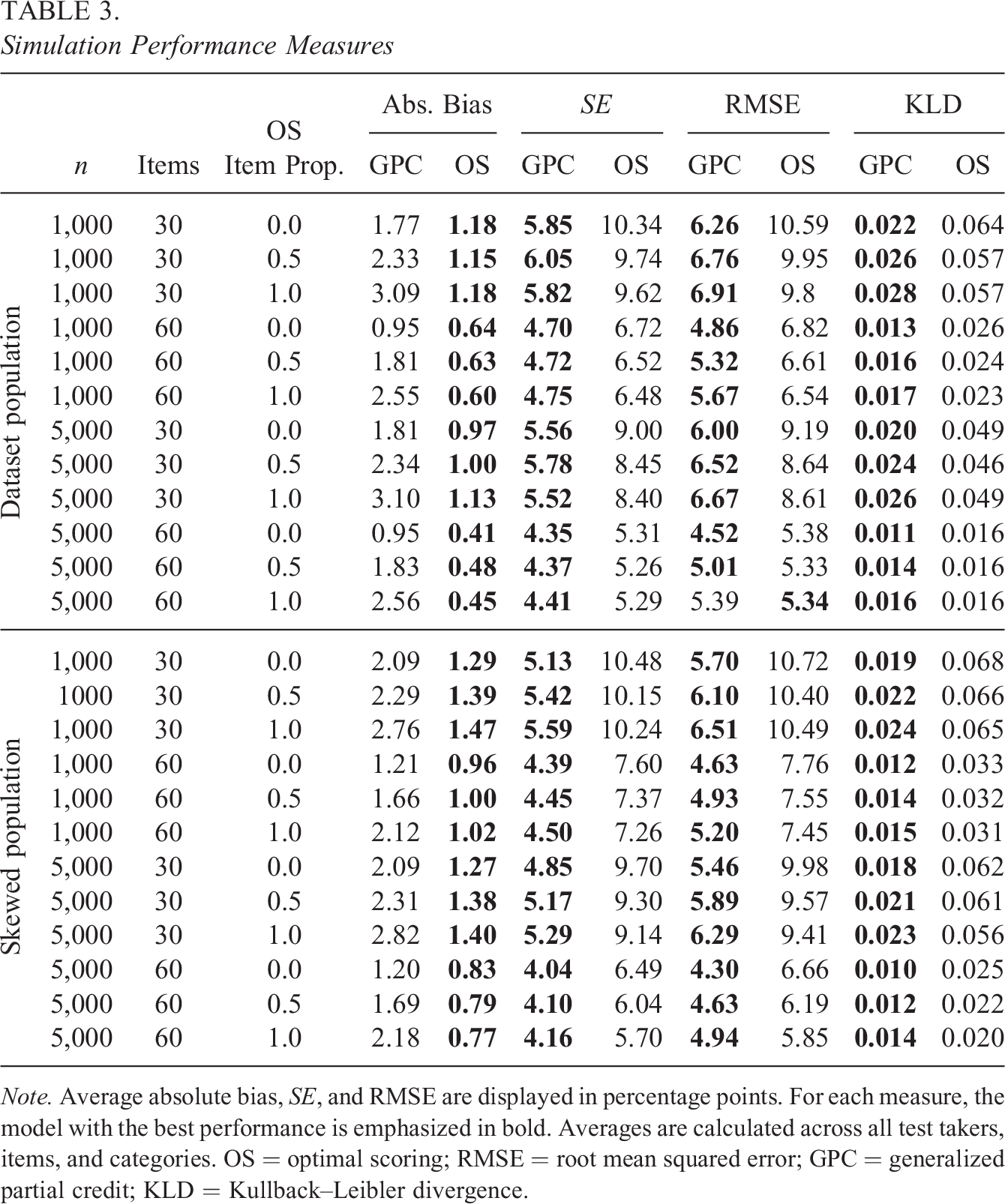
Note. Average absolute bias, SE, and RMSE are displayed in percentage points. For each measure, the model with the best performance is emphasized in bold. Averages are calculated across all test takers, items, and categories. OS = optimal scoring; RMSE = root mean squared error; GPC = generalized partial credit; KLD = Kullback–Leibler divergence.
Table 3 shows the performance measures in Algorithm 2 for each method averaged over test takers, items, and item scores. As the total probability bias averaged over all item categories always sum to zero, the bias entries in the table were computed using the absolute values of the bias estimates retrieved using Equation 10. The results from using 10,000 test takers are omitted, as only slight reductions in bias and SE were observed. It is worth highlighting the importance of low bias, as it is crucial for accurate estimation of IRFs and test scores, and the OS model excels in this aspect. In all simulated scenarios, the OS model exhibited a smaller average absolute bias compared to the GPC model, including scenarios where the true IRFs adhered to the parametric shape of the GPC model. The GPC model shows larger bias when more OS items are used for data generation, while the bias from the OS model is more similar in size no matter if OS or GPC items are used to generate data. The bias is close to the same for all sample sizes for both models, but a slight decrease in bias is shown when using OS as the sample sizes increases, provided other parameters are kept the same. However, the OS model has larger average SEs compared to the GPC model, and the decrease in bias does not compensate for the increase in SE when evaluating performance using measures, such as RMSE and KLD, with the exception of the scenario where all items were generated using the OS model and a sample size of 5,000. Increasing the sample size has a marginal effect on reducing average SE when comparing scenarios with the same number of items and proportion of true OS items. In contrast, adding more items leads to substantial improvements in SE, RMSE, and KLD, with the effect on SE being more pronounced for the OS model compared to the GPC model.
Having a skewed population does not have a large effect on any performance measure. One should note that these are average measures computed only for each test takers sampled from the skewed/data set population matching the scenario. Figure 7 plots the resulting bias and RMSE from each model against the true percentile arc length
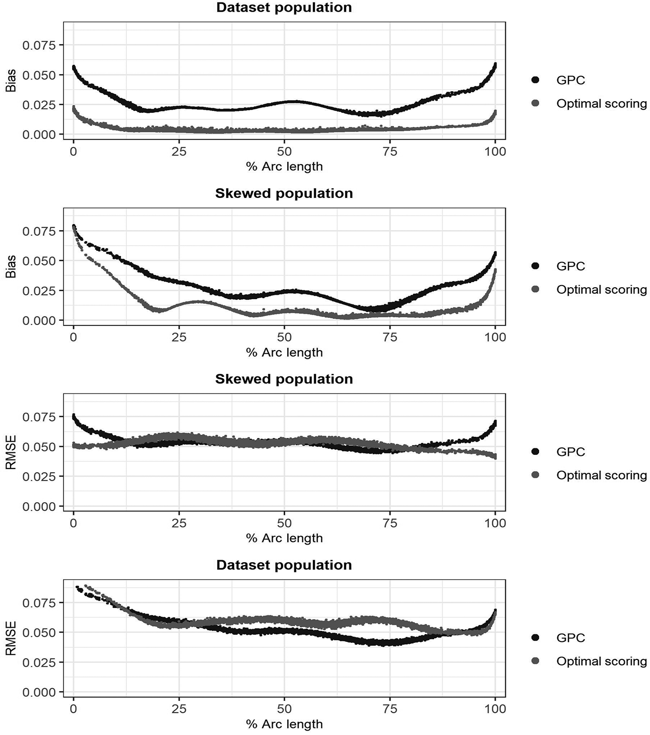
Item response functions probability absolute bias and root mean squared error averaged over all items and item scores plotted against % arc length.
It is clear from Figure 7 that the bias is larger for high and low scoring test takers. Having a left skewed population results in larger bias for low scorers. This is expected, as fewer test takers are found closer to the lower
7. Discussion
The aim of this study was to investigate whether the OS model is preferable to the GPC model in terms of model fit and to showcase the efficacy of the arc length
A key feature of arc length is its invariance to the arbitrary choice of latent trait
In terms of model fit, the OS model showcased a superior fit for multiple polytomously scored items, some examples shown in Figures 3 and 4. These results are in line with previous studies, where OS was compared against parametric alternatives on tests using dichotomous test items (Ramsay & Wiberg, 2017; Wiberg et al., 2019). When comparing model fit to real test data using CV LL and the binning method as described in Section 5.3, OS also showed promising results. OS models with similar or better performance than the GPC model could always be found by tweaking the OS model parameters. However, the process of finding the appropriate number of bins, knots, and the appropriate spline order for the data at hand can be cumbersome and using a more flexible model can lead to overfitting. This was especially true for the Swedish SAT data sets despite the large sample sizes, while the results for models fit to the national mathematics data sets were more conflicting.
One should consider the fact that the test items in the Swedish SAT forms are constructed by experts in test construction and the items are thoroughly tested before being included in an administered test form to the general public. This process should generally lead to items being more closely related to the latent construct(s) the test is aimed to measure and produce items that are more likely to be responded to correctly by the more able students. Despite the inherent simplification of reducing the responses from all items to a single construct, this could be a potential explanation to why, for most items in the data, the estimated IRFs behave in a lenient way, where the probabilities for correct responses monotonically increase with test taker ability. These properties should generally favor simpler parametric models such as the GPC. For other tests where the relationship between item scores and test taker ability is more complex, the benefits of using a nonparametric approach such as OS would most likely be even larger.
Fitting OS models using splines without knots proved to be efficient in this study. In previous research on OS, more flexible spline functions were used. For example, Ramsay et al. (2020) used 18 bins in conjunction with order 5 spline functions and two knots to analyze a 473 sample from the symptom distress scale, a 13 item rating scale form measuring distress in cancer patients. Ramsay et al. (2019) used 53 bins with 24 basis functions to analyze Swedish SAT data. On the contrary, previous studies also applied a roughness penalty on the third derivatives of each spline to prevent overfitting. For this study, the use of penalized smoothing splines resulted in worse performance in terms of the empirical model evaluation measures, and the results were thus omitted. Further research should be conducted on how to obtain a suitable amount of smoothing in a practical way.
It is important to strike a balance between bias and variance when choosing a model, as a model with low bias but high variance can lead to overfitting, while a model with high bias but low variance can fail to model the actual relationship between the underlying ability and the item responses. Through our simulation study, we showed that fitting an OS model results in smaller IRF probability bias compared to fitting a GPC model. As with many nonparametric approaches, this comes with the cost of larger SEs. The GPC model outperformed OS in terms of KLD and item response probability recovery RMSE in most simulated scenarios. Looking at the simulations, it appears one would need large samples containing thousands of test takers in combination with a large number of test items to really reap the benefits of the bias reduction from the nonparametric curve estimation for tests such as the Swedish SAT. However, small bias is often considered more important than small SE. In situations where the RMSE and/or KLD from two competing models are somewhat similar, one may argue that it is more fair that someone gets a different score than they should by chance from larger SEs than by bias from choosing a specific parametric model.
We recognize the assumption of unidimensionality as a limitation of the current study. In reality, multiple abilities often come into play during an exam. While this study did not address multidimensional abilities, we are actively working to extend the OS IRT methodology to handle such scenarios, while maintaining the benefits of our proposed approach. Future publications will provide insights into these multidimensional extensions. In the meantime, readers should interpret our findings in the context of a unidimensional
Overall, OS proves to be a viable alternative to parametric IRT for analyzing test data containing polytomously scored items. Especially for tests containing a large number of test items in combination with large sample sizes. In future studies, it would be of interest to compare OS with other recently introduced nonparametric/semiparametric IRF estimation methods. Examples include Bayesian nonparametric methods (Arenson & Karabatsos, 2018; Duncan & MacEachern, 2008), the monotonic polynomial method (Falk & Cai, 2016; Liang & Browne, 2015) or the approach of using a mix of parametric and nonparametric curves for different items implemented in the
Supplemental Material
Supplemental Material, sj-docx-1-jeb-10.3102_10769986231207879 - Analyzing Polytomous Test Data: A Comparison Between an Information-Based IRT Model and the Generalized Partial Credit Model
Supplemental Material, sj-docx-1-jeb-10.3102_10769986231207879 for Analyzing Polytomous Test Data: A Comparison Between an Information-Based IRT Model and the Generalized Partial Credit Model by Joakim Wallmark, James O. Ramsay, Juan Li and Marie Wiberg in Journal of Educational and Behavioral Statistics
Footnotes
Declaration of Conflicting Interests
The author(s) declared no potential conflicts of interest with respect to the research, authorship, and/or publication of this article.
Funding
The author(s) disclosed receipt of the following financial support for the research, authorship, and/or publication of this article: The research was funded by the Swedish Wallenberg MMW 2019.0129 grant.
Note
References
Supplementary Material
Please find the following supplemental material available below.
For Open Access articles published under a Creative Commons License, all supplemental material carries the same license as the article it is associated with.
For non-Open Access articles published, all supplemental material carries a non-exclusive license, and permission requests for re-use of supplemental material or any part of supplemental material shall be sent directly to the copyright owner as specified in the copyright notice associated with the article.