Identifying Informative Predictor Variables With Random Forests

Abstract

Random forests are a nonparametric machine learning method, which is currently gaining popularity in the behavioral sciences. Despite random forests’ potential advantages over more conventional statistical methods, a remaining question is how reliably informative predictor variables can be identified by means of random forests. The present study aims at giving a comprehensible introduction to the topic of variable selection with random forests and providing an overview of the currently proposed selection methods. Using simulation studies, the variable selection methods are examined regarding their statistical properties, and comparisons between their performances and the performance of a conventional linear model are drawn. Advantages and disadvantages of the examined methods are discussed, and practical recommendations for the use of random forests for variable selection are given.

One of the most notable trends in current research is the increasing use of machine learning techniques for data analysis. In addition to the fields of technology and life sciences, where machine learning has already become an established tool, it is the behavioral social sciences where machine learning is currently spreading. As a consequence, more and more behavioral scientists have become interested in the possibilities and advantages machine learning might have to offer. The surge in machine learning’s popularity is due to a range of positive characteristics which machine learning models comprise. For example, one often cited benefit is the ability to deal with high-dimensional data, including data in which there are more predictor variables than observations (“ $n<p$ ” case). By contrast, many classically used methods, such as linear regression models, cannot be applied in such a setting.

Random forests stand out as a machine learning method that received particularly positive interest. First introduced by Breiman (2001), random forests are a supervised learning method and can as such be used for the prediction of a response variable (y) based on a potentially large number of predictor variables (x ₁,…, x_p ). Apart from being able to deal with high-dimensional data, random forests combine a series of attractive traits. Random forests are a completely nonparametric method and, therefore, do not pose any requirements to the distribution of the data. They can be applied to classification problems (categorical response variable) as well as to regression problems (numerical response variable) and also to survival data (Hothorn et al., 2005; Ishwaran et al., 2008). One trait especially attractive for researchers without machine learning experience is the notion that random forests work well “out-of-the-box.” Working “out-of-the-box” implies that even without parameter tuning random forests tend to achieve good performance but typically not overfit, thus allowing a quick and uncomplicated application.

The positive characteristics of random forests have led to them being picked up by a multitude of fields. Especially in epidemiology, genetics, and medicine, random forests have become increasingly popular (Touw et al., 2013). Interestingly, there has also been an increasing number of attempts to apply random forests to the study of human behavior and cognition. Examples stem from various areas of research, such as the analysis of neuroimaging data from MRI and EEG (electroencephalogram) measurements (Mesaros et al., 2012; Shen et al., 2007), performance prediction in education research (Gutiérrez et al., 2019), the behavioral screening of drivers for accident prevention (Harb et al., 2009; Martensson et al., 2019), the classification of psychiatric disorders (Brancati et al., 2019; Walsh-Messinger et al., 2019), sleep research (Kaplan et al., 2017), and linguistics (Fonteyn & Nini, 2020). Although high-dimensional data sets are less prevalent in behavioral research, some of the listed examples illustrate cases in which such data can appear. Measuring neural activity through fMRI or EEG, for example, can result in the accumulation of a high number of time-, location-, and frequency-specific variables. Another potential source of high-dimensional data are large panel studies or generally studies employing extensive questionnaires (Pargent & Albert-von der Gönna, 2018). However, random forests are not limited to the case of “ $n<p$ ”, but can also be applied to smaller, more conventional data sets. Even under these circumstances, random forests can exhibit some advantages over classical statistical methods. The main advantage lies in random forests’ ability to flexibly detect complex patterns in data, which might not be covered by a simple linear model. Consequently, random forests often outperform classical statistical methods in terms of predictive performance (Couronné et al., 2018).

The Random Forest Algorithm

Since it is not in the scope of the present manuscript to give an extensive description of the random forest algorithm, only an abbreviated introduction to random forests is provided. For a more detailed discussion, we refer the reader to Strobl et al. (2009).

In order to describe random forests, it is necessary to first cover their basic building block, the “decision tree” (also referred to as classification and regression trees). A decision tree is a predictive model in the shape of a flowchart and can best be illustrated by an example. To this end, an artificial data set, loosely inspired from the field of sleep research, was generated. The hypothetical data consisted of the continuous response variable sleep quality and the six artificial predictor variables caffeine use (mg per day), smoking status, body mass index, socioeconomic status, anxiety, and education. Figure 1 shows a decision tree created with the R-package partykit based on the artificial data.

Figure 1.

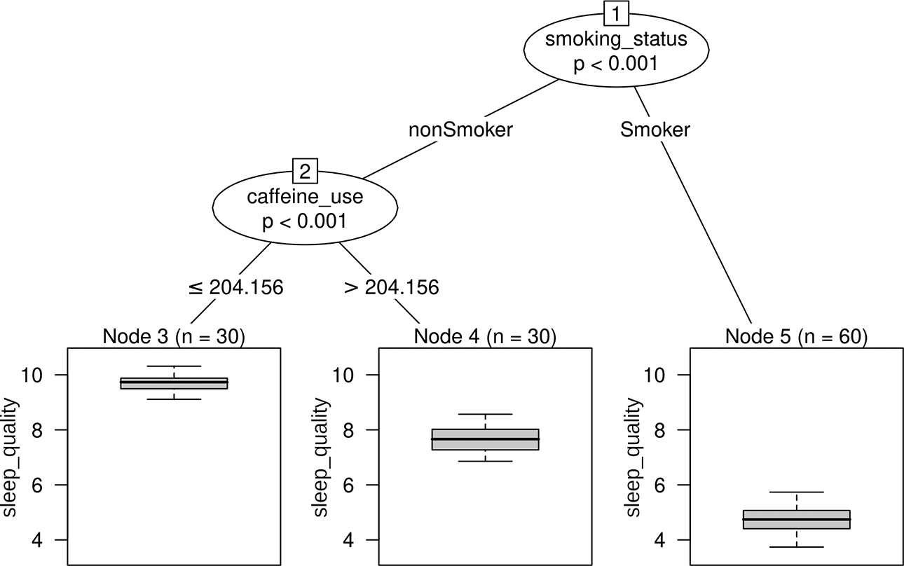
Simple decision tree (regression tree) based on the artificial sleep quality data.

The structure of the decision tree in Figure 1 reveals that the pattern in the data can be described by two splits. In a first split, the sample is separated into people who smoke and people who do not smoke. For persons who fall to the left side of the first split (“nonSmoker”), a second split is performed along the variable caffeine use (separating observations up to and above a daily caffeine consumption of 204.16 mg). The boxplots in the terminal nodes depict the distribution of sleep quality values in the corresponding group of persons. To predict the sleep quality of a new person, they are “run through” the decision tree starting at the top. Classically, the mean sleep quality in the respective terminal node a person falls into is used for prediction. Due to decision trees’ flowchart-like structure, it is possible to visually retrace each step leading up to a prediction. This facilitates the interpretation of the model, a feature which is regarded as one of decision trees’ main advantages. For the hypothetical decision tree in Figure 1, one could, for example, conclude that the sleep quality of a person is lowest if a person smokes, and for nonsmokers, the sleep quality is further affected by the daily caffeine consumption. It has to be noted, however, that the artificial data underlying the decision tree in Figure 1 were purposely created with a simple structure. When facing a more complex data pattern, interpreting the resulting decision tree becomes increasingly more complex, too. The algorithm responsible for building a decision tree is known as “recursive partitioning.” The goal in recursive partitioning is to separate the data using sequential, typically binary splits, so that the persons within each created subgroup are similar to each other in terms of the response variable. The algorithm has to repeatedly identify the variable best suited for splitting and, once the variable is selected, identify the best splitting point along that variable. When looking again at the decision tree in Figure 1, it is evident that the tree only selected the two variables smoking status and caffeine use for splitting. The remaining variables did not further improve the splits and were therefore not selected by the tree.

As hinted at by the name, random forests work by creating an ensemble of decision trees (Breiman, 2001). In order to generate multiple decision trees (e.g., 500 or 1,000 trees in total), a large number of random bootstrap samples (subsamples drawn with replacement) are drawn from the available data. Each drawn sample is used to build one decision tree. Additionally, in each node of a tree, only a random sample from all predictor variables is made available for splitting. Due to the differences in the random samples and the selected splitting variables, the resulting trees typically vary in their structure. Figure 2 shows the first three decision trees of a random forest built with our artificial data. When predicting the sleep quality of a new person, the person’s data are passed through each decision tree of the random forest. The prediction of each tree is recorded and a pooled estimate is generated for the final prediction (e.g., using the average prediction over all trees).

Figure 2.

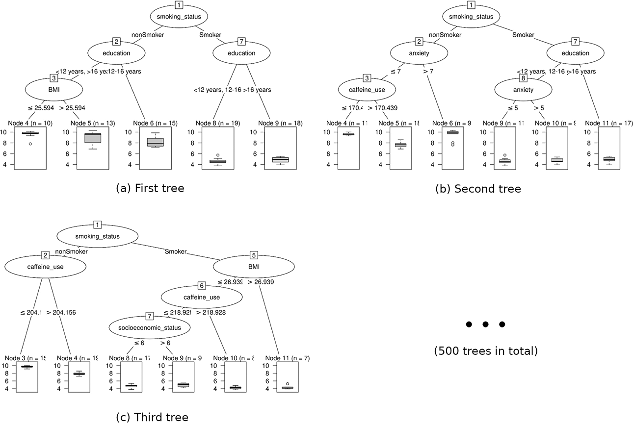
The structure of the first three decision trees of a random forest model based on the artificial sleep quality data.

The “shuffling” of first the available data and second the available predictor variables in random forests has been shown to positively affect performance (Breiman, 2001; Ho, 2002). As an intuitive explanation, one can imagine the case where a subtle predictor of the response variable is not selected for splitting in a single decision tree, because it is trumped by more dominant predictors. In a random forest, however, some trees will be encouraged to use this variable since the random sample of possible splitting variables does not include the more dominant predictors. Thus, the random forest allows a wider range of potentially covert relations to participate in the prediction process. On a more technical note, the sampling procedures in random forests help to achieve smooth and stable decision boundaries, which addresses some of the main caveats when using single decision trees.

A general concern in predictive modeling is the evaluation of a model’s predictive performance, that is, how good the model can predict the response variable for new observations. Random forests come with their own integrated measure of performance, the out-of-bag (OOB) error (Breiman, 2001). Since the individual trees of a random forest are built using bootstrap samples, it follows that each decision tree is only exposed to a fraction of the original data. The observations which the tree has not been exposed to are referred to as a tree’s OOB observations. To calculate the OOB error, the random forest is used to predict the response variable for each observation, but only using trees for which an observation is OOB. This procedure is supposed to simulate the prediction of new, unknown data similar to an assessment with cross-validation. The final OOB error can be calculated as the mean squared error when predicting observations in the described fashion (or the misclassification rate in the setting of classification).

The Issue of Interpretability

Despite their positive characteristics, random forests do suffer from certain drawbacks. One central issue is their restricted interpretability. Random forests do convey the feeling of a “black box,” which is a shared characteristic among many machine learning methods, including, for example, neural networks. The “black box” analogy becomes evident when inspecting the random forest partly shown in Figure 2. It is unfeasible to visually examine and overview the structure of all 500 trees. As a consequence, it remains unclear what exact roles the individual predictor variables play and which of them importantly relate to the response variable.

Such a lack of immediate insight stands in stark contrast to the interpretability of parametric models, such as linear or logistic regression models. A regression model returns a regression coefficient for each predictor variable. A variable’s regression coefficient represents the estimated slope of the variable’s partial linear relation with the response variable. The interpretation of a regression coefficient is straightforward: With a positive coefficient, the response variable is expected to be higher for higher predictor values, while with a negative coefficient, the response variable is expected to be lower for higher predictor values. Moreover, statistical tests are available to formally testing whether a regression coefficient is significantly different from zero. Thus, a regression coefficient conveys information about the strength of a relation through its size, the direction of a relation through its sign, and the statistical significance of a relation through its p value.

The relatively young branch of “interpretable machine learning” involves the development of strategies to penetrate the “black box” property of complex machine learning methods (Murdoch et al., 2019). One commonly used tool to improve interpretation are variable importance scores. The general intuition behind a variable importance score is to quantify the contribution of a variable when predicting the response variable. By distinguishing strongly contributing variables from weakly contributing variables, the goal is to identify the predictors, which do bear a meaningful relation with the response variable (from here on referred to as “informative” predictors). Therefore, variable importance scores can, similar to coefficients in a linear model, give an indication of strong or weak relationships between a predictor and the response variable.

There have been different proposals how importance scores should be calculated for random forests. One widely used statistic is the permutation importance. The rationale behind the permutation importance is to examine how a specific predictor variable is affecting a random forest’s overall predictive performance. After a random forest has been fitted and its predictive accuracy computed (e.g., by the OOB error), the values of the predictor variable of interest are permuted in the data set. Now, the predictive accuracy of the random forest is again assessed using this new, permuted data set, and the performance before and after permutation is compared (e.g., by taking the difference between the two resulting OOB errors). Assuming that the predictor has an informative relation with the response variable, permuting its values is expected to break up this relation and to cause a drop in prediction accuracy. On the other hand, assuming that the predictor does not have an informative relation with the response variable, permuting its values should not systematically change the performance of the random forest. As a result, permutation importances of zero (or values close to zero) indicate no association between a specific predictor and the response variable, while large positive permutation importances indicate that the predictor was relevant for predicting the response. It is also possible for a variable to end up with a small negative permutation importance. This is the case when randomly permuting the values of a predictor leads to an improved predictive performance by chance and is hence also indicative of no association between the predictor and the response variable. Figure 3 visualizes the permutation importance scores based on the artificial sleep quality data.

Figure 3.

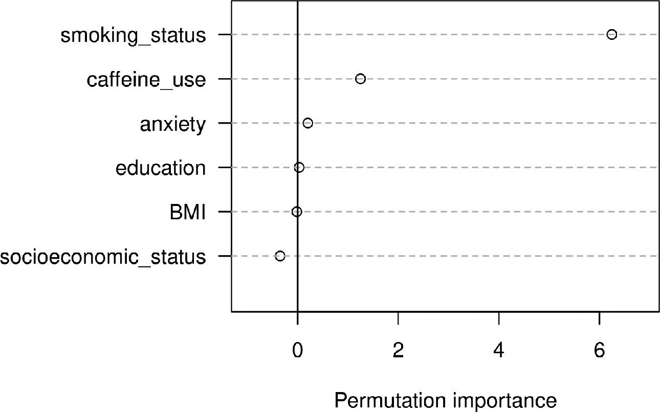
Variable importance scores from the random forest based on the artificial sleep quality data.

In summary, the permutation importance offers a way to assess the strength of a predictor’s relation with the response variable. It has to be noted, however, that permutation importances are not based on solid statistical theory but rather represent a heuristic approach to evaluate a predictor’s impact in a model. In particular, the permutation importance does not inform about the direction or shape of a predictor’s relation with the response variable. It is merely an indication that there is some kind of connection between the two variables. The connection could, for example, be a positive relation, a negative relation, a nonlinear relation, or even a complex higher order interaction in which the predictor is involved.

Significant Versus Nonsignificant Importance

A crucial aspect of importance scores is their evaluation. Since permutation importances take on values on a continuous scale, it is not apparent at which threshold, a score truly reflects a meaningful effect and is not merely the result of chance. Without a way to judge whether an importance score is significantly larger than what would be expected by chance, the concept of variable importance is of limited use to many researchers. In the literature, there is a range of proposals how to perform such an evaluation. Some of the proposals include very simple, heuristic approaches. One such example constitutes the rule of thumb introduced by Strobl et al. (2009). The idea behind this approach is to compare the importance scores of all predictors to the largest negative importance score achieved. The largest negative importance score is conceived as an expression of the extent to which an uninformative variable’s score can vary around zero by chance alone. Accordingly, only variables with an importance score surpassing the absolute value of the largest negative score are labeled as potentially interesting. While this approach was originally introduced as a mere rule of thumb, later publications have erroneously termed variables selected with this approach as “significant.”

To date, a multitude of more elaborate evaluation tools have been proposed by various researchers. The suggested methods can be broadly divided into two main categories: performance-based methods and test-based methods (Hapfelmeier & Ulm, 2013). The two categories differ in their strategy of identifying informative predictors. While performance-based methods use the model’s predictive performance for variable selection, test-based methods conduct a statistical test on the variables’ importance scores.

Which Variable Selection Method to Choose?

Given the double-digit number of the proposed methods for variable selection in random forests (Speiser et al., 2019), the question arises which of the techniques one should choose. The goal of the present study is to give a basic understanding of how the respective methods work and to display the advantages and disadvantages associated with them. Further, the present study uses simulated data to examine and compare the statistical properties of the variable selection techniques. Unsurprisingly, this is not the first comparison study conducted on the topic. To give an overview of comparable studies, Table 1 displays a selection of the most extensive comparison studies published. Previous publications have predominantly approached the subject of variable selection in random forests from the biostatistics corner, with a strong focus on genetics (Degenhardt et al., 2019; Szymczak et al., 2016). As a result, comparison studies mainly focused on the type of data typically encountered in similar fields, often including a very large number of predictors or observations. In addition, the focus of previous studies was mainly on prediction, that is, judging the variable selection tools based on the predictive performances achieved when including the selected variables in a final model (Gazzola & Jeong, 2019; Sanchez-Pinto et al., 2018; Speiser et al., 2019). In contrast, the present study focuses on data settings that will realistically occur in psychological and social science research, namely, moderate numbers of variables and sample sizes, combined with different amounts of truly informative variables, as well as settings with correlations and interaction effects. Data sets of this latter type are used to highlight differences in the properties of random forest-based variable selection and (generalized) linear modeling approaches. Also, the present study focuses not primarily on prediction accuracy but on further statistical properties of the variable selection methods, such as the selection rates of truly informative and uninformative variables.

Table 1.

Summary of Previous Comparison Studies

				Comparison Studies
Method Reference Strategy				Speiser et al.(2019) Setting (Classification) Real data:max 1,000 varsmax 1,000 obs Evaluation Pred. performance	Degenhardt et al.(2019) Setting (Class. & Regr.) Real data:max ˜22,000 varsmax ˜500 obs Simulated data:max 5,000 varsmax 200 obs Evaluation Pred. performanceStat. properties	Gazzola & Jeong(2019) Setting (Class. & Regr.) Real data:max ˜5,600 varsmax ˜500 obs Simulated data:max 77varsmax 400 obs Evaluation Pred. performance	Sanchez-Pintoet al. (2018) Setting (Classification) Real data:max 29 varsmax ˜270,000 obs Evaluation Pred. performance	Hapfelmeier &Ulm (2013) Setting (Class. & Regr.) Real data:max 22 varsmax ˜500 obs Simulated data:max 20 varsmax 100 obs Evaluation Pred. performanceStat. properties
Perf.-based	varSelRF	Díaz-Uriarte & Alvarez de Andrés (2006)	Stepwise selection	✓	✓	✓	—	✓
	VSURF	Genuer et al. (2010)		✓	—	✓	✓	✓
Test-based	PIMP	Altmann et al. (2010)	Randomization test	✓	✓	✓	—	✓
	Hapfelmeier	Hapfelmeier & Ulm (2013)		✓	—	✓	—	✓
	Boruta	Kursa & Rudnicki (2010)		✓	✓	✓	✓	—
	Janitza	Janitza et al. (2018)	Mirror negative imp. scores	✓	✓	—	—	—
	Ishwaran	Ishwaran & Lu (2019)	Bootstrap estimator	—	—	—	—	—
Other	redLine	Strobl et al. (2009)	Use smallest imp. score as benchmark	—	—	—	—	—
	r2VIM	Szymczak et al. (2016)		—	✓	—	—	—
Summary				The authors recommend VSURF. For large data sets, varSelRF and Boruta are recommended	The authors recommend Janitza and Boruta	Boruta shows good overall performance	Boruta and VSURF show good performance	PIMP and Hapfelmeier best control false alarm rates. The authors overall recommend Hapfelmeier

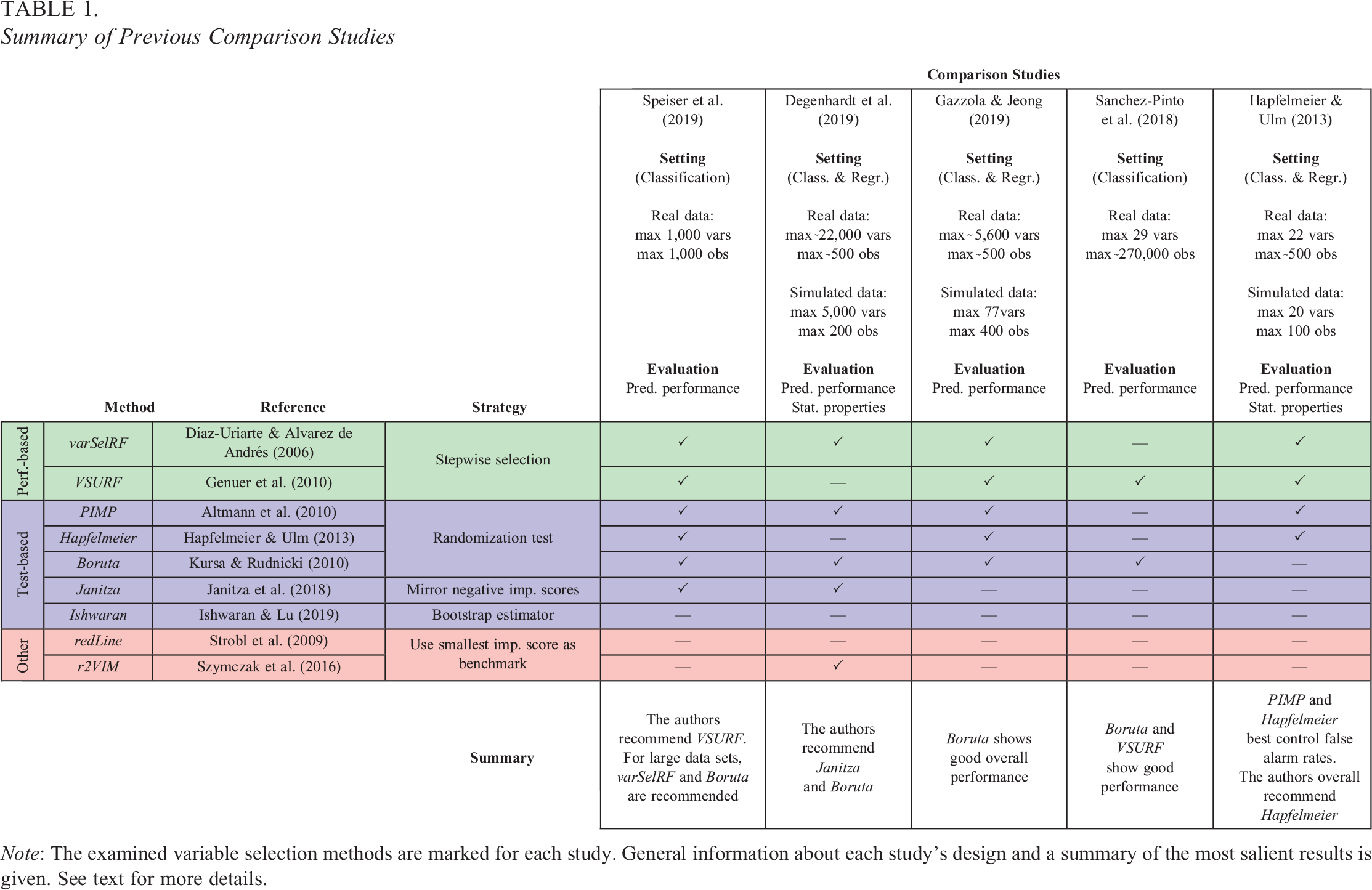
Note: The examined variable selection methods are marked for each study. General information about each study's design and a summary of the most salient results is given. See text for more details.

The reason for setting the focus on selection rates instead of prediction accuracy lies within the target audience of the present manuscript. Since for many researchers in the social sciences interpretation is a more central concern than mere prediction accuracy, it can be expected that the presented methods will be applied within such a context. Especially since some methods return empirical “p values” for individual predictors, researchers might be tempted to interpret results in the same fashion they are used to from parametric modeling procedures. Investigating the selection rates of informative and uninformative variables in our simulations serves as a reality check as to what kind of behavior researchers actually have to expect from the discussed methods.

Variable Selection Methods

In total, nine variable selection methods for random forests were examined. All included selection procedures are available in the open-source software R for statistical computing (R Development Core Team, 2022). The methods included two performance-based approaches, five test-based approaches, and two other approaches, which do not fit into the former two categories. In the following sections, the rationale behind the three classes of approaches is presented. Taking the manuscript’s length into consideration, the detailed descriptions of the individual methods were moved to the Online Supplementary Material of the manuscript. The descriptions in the Online Supplementary Material also include potential adaptations when applying these methods in a classification instead of a regression setting.

Performance-Based Methods

As the name suggests, performance-based methods focus on a model’s predictive performance to distinguish informative from uninformative variables. The general intuition behind performance-based methods is that the removal of uninformative variables should not impair the prediction accuracy of the model (classically measured by the OOB error). Thus, the goal in performance-based methods is to reduce the number of predictors, while retaining (or even reducing) the OOB error. The ideal performance-based method would iterate through all possible combinations of predictors and select the set of predictors, which results in the smallest, best-performing model. However, with an increasing amount of variables, it becomes less feasible to compare all variable subsets due to the exponentially growing number of possible configurations. Therefore, performance-based methods usually apply a stepwise procedure, based on the variables’ permutation importances, to efficiently test appropriate combinations of predictors. Once the best-performing (or close to best performing) model is found, all variables which are part of this model are labeled as informative, while the variables which did not make the selection are labeled as uninformative.

The two examined performance-based methods in the present study were varSelRF by Díaz-Uriarte and Alvarez de Andrés (2006) and VSURF by Genuer et al. (2010). Although both methods aim at finding a small predictor subset while retaining good prediction accuracy, they differ in their strategy of iterating through possible combinations of predictors.

Test-Based Methods

Test-based methods take an approach stimulated by formal hypothesis testing to the task of identifying informative predictors. The goal in test-based methods is to tackle the null hypothesis that a specific variable has no relation with the response variable. Typically using a randomization test framework, test-based methods try to reproduce the distribution of a variable’s importance score under the null hypothesis, which allows the computation of associated one-sided p values. Following the conventional procedure in hypothesis testing, variables with p values below a certain significance level (typically 5%) are regarded as having an importance score significantly larger than zero and are consequently labeled as informative.

The five examined test-based methods include PIMP by Altmann et al. (2010), the approach proposed by Hapfelmeier and Ulm (2013; from here on referred to as Hapfelmeier), Boruta by Kursa and Rudnicki (2010), the approach proposed by Janitza et al. (2018; from here on referred to as Janitza), and the approach proposed by Ishwaran and Lu (2019; from here on referred to as Ishwaran). The five methods can be divided into three subgroups based on their operating principles. The first group contains PIMP, Hapfelmeier, and Boruta. These three approaches rely on permutation schemes to map the null distribution of importance scores. In contrast, the Janitza method uses negative importance scores to approximate the null distribution. Lastly, the Ishwaran method estimates the confidence intervals of a variable’s importance score using a bootstrap estimator.

Other Methods

The group of “other” methods comprises variable selection techniques, which do not clearly belong to either of the previous two categories. Two such methods were examined: The heuristic introduced by Strobl et al. (2009; from here on referred to as redLine, because in many applications, a red line is used to visualize this rule of thumb) and r2VIM by Szymczak et al. (2016). Both procedures rely on the largest negative importance score to identify informative predictors.

Simulation Studies

The simulations were divided into two parts, Study I and Study II. In each study, the variable selection methods were evaluated under multiple conditions. All simulations were performed using the statistical software R (R Development Core Team, 2022, v4.1.3). To fit random forests, the randomForest function of the identically named R-package was used. It is known that the randomForest function has an inherent preference for specific types of splitting variables (specifically variables with many cutpoints). This affects the variance of the resulting permutation importances (Strobl et al., 2007) and carries over to variable selection methods based on importance rankings, as we will show in the following. The cforest function of the R-package party (or partykit) is recommended as a bias-free alternative (Hothorn et al., 2006). However, since some of the applied variable selection methods are based on the randomForest package, it was used throughout the study to allow the comparison between methods. For methods that allowed a transfer to the cforest function, all simulations were run with both functions. Both simulation studies were performed in a regression as well as a classification setting. Due to the resemblance of results between the two settings, however, only the regression setting is presented in the main manuscript. The details and results of the classification setting are included in the Online Supplementary Material. Random forests were always generated using 500 decision trees (ntree $=500$ ). In each node, the total number of predictors divided by three was used as the number of randomly evaluated variables for splitting (mtry argument), which is the default mtry value for regression in the randomForest function. The following sections describe the content and structure of the two simulation studies.

Study I

In the first simulation study, the statistical properties of the variable selection methods were examined under fairly simple conditions. Study I comprised two substudies, Study IA and Study IB, whose settings are described in the following.

Simulation setting (Study IA)

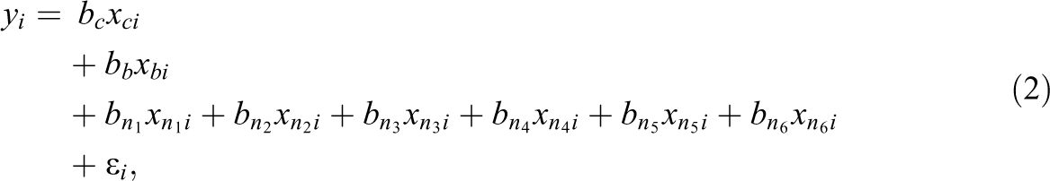
In Study IA, the artificial data consisted of a numerical response variable (y) and multiple numerical predictor variables (x_i ). The predictor variables were independently sampled from a standard normal distribution and were, therefore, not correlated with each other. Among the predictor variables, we distinguished between “informative” and “uninformative” variables. Informative variables were the predictors, which did contribute to the generation of the response variable y, while uninformative variables were not involved in the generation of y. The values of y were created according to a linear regression model, in which, consequently, only the informative variables were included. Equation 1 shows the regression equation for the first of three conditions simulated in Study IA. The conditions differed only in the numbers of informative and uninformative variables. Condition 1 included 21 predictor variables of which 18 were uninformative and 3 were informative. It can be seen in Equation 1 that the three informative predictor variables acted on the response variable with three different effect sizes (“weak,” “medium,” and “strong” effect) and were, therefore, not equally “important”:

$y_i=b_w{x}_{1i}+b_m{x}_{2i}+b_s{x}_{3i}+{\text{∊}}_i,$

1

with:

${\text{∊}}_i\stackrel{i\mathrm{.}i\mathrm{.}d}{\sim }\mathcal{N}(0,16),$

$x_1,x_2,x_3:\text{informative variables,}$

$b_w=0.8,b_m=1,\text{and }{b}_s=\mathrm{1.2.}$

Condition 2 also included 21 predictor variables, but 3 of which were uninformative and 18 were informative. Condition 3 included 210 predictor variables, of which 180 were uninformative and 30 were informative. The generation of y in the second and third conditions followed the same general pattern as in Condition 1, that is, the informative variables were divided into three, equally sized groups of “weak,” “medium,” and “strong” predictors. ¹ The effect sizes of 0.8, 1, and 1.2 and an error variance of 16 were selected since they were found in prestudies to adequately prevent ceiling or floor effects in the methods’ achieved detection rates.

The reason for including the described three conditions in Study IA was to get an impression of how the variable selection methods performed in a straightforward linear regression setting and to examine the effect of the number of informative and uninformative variables on their performance. Since several of the variable selection methods rely on the presence of uninformative variables (see “Variable Selection Methods” section), there is a reason to suspect that performance is affected by the ratio of informative to uninformative predictor variables in the data.

In each simulation, a training data set consisting of 200 observations was generated 1,000 times (with the exception of Condition 3, in which due to the ten-fold higher number of variables, 100 simulations were performed to reduce computation time). The following outcomes were examined for each selection method: (1) mean false alarm rate: the proportion of uninformative variables, which were wrongly labeled as informative, averaged over the simulation repetitions; (2) mean detection rate: the proportion of informative variables, which were correctly labeled as informative (separately recorded for weak, medium and strong predictors), averaged over the simulation repetitions; (3) mean test error of the final random forest: in each simulation, a test data set of the same size as the training data was generated. The test error describes the mean squared error when predicting the response variable in the test data set using the final random forest. The final random forest is based on the training data and only includes the variables selected by the selection method; and (4) computation times (collected for each simulation round). ²

For the first two conditions, a linear regression model was also estimated in order to allow the comparison between the performance of the random forest variable selection and the results of the linear model. In Condition 3, the linear model was not included since it was not identifiable given the number of 210 predictors with 200 observations. For the linear regression model, the significance of each variable’s coefficient (based on the t-statistic) was used as the variable selection criterion.

Results (Study IA)

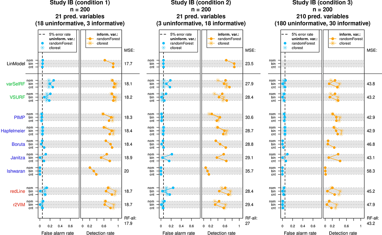
The results of Study IA are displayed in Figure 4. Figure 4 consists of three graphs, each depicting the results of one condition. The examined methods are listed vertically on the left-hand side and colored according to the class of methods they belong to (performance-based, test-based, and other). Each method’s results are displayed on the corresponding row. For each condition, the achieved mean false alarm rates are displayed in the left panel (blue points) and the achieved mean detection rates displayed in the right panel (orange points). For each method, the mean detection rates corresponding to the three types of predictors (weak, medium, and strong) are connected to a line. Following conventions in hypothesis testing, the ideal method should always adhere to a fixed false alarm rate of 5% (dashed line) while maintaining high detection rates. Therefore, the blue point of a method should ideally lie as close as possible to the dashed line. The orange line on the other hand is expected to show an upward trend due to the larger effect sizes and should ideally lie as much to the right as possible, indicating high detection rates.

Figure 4.

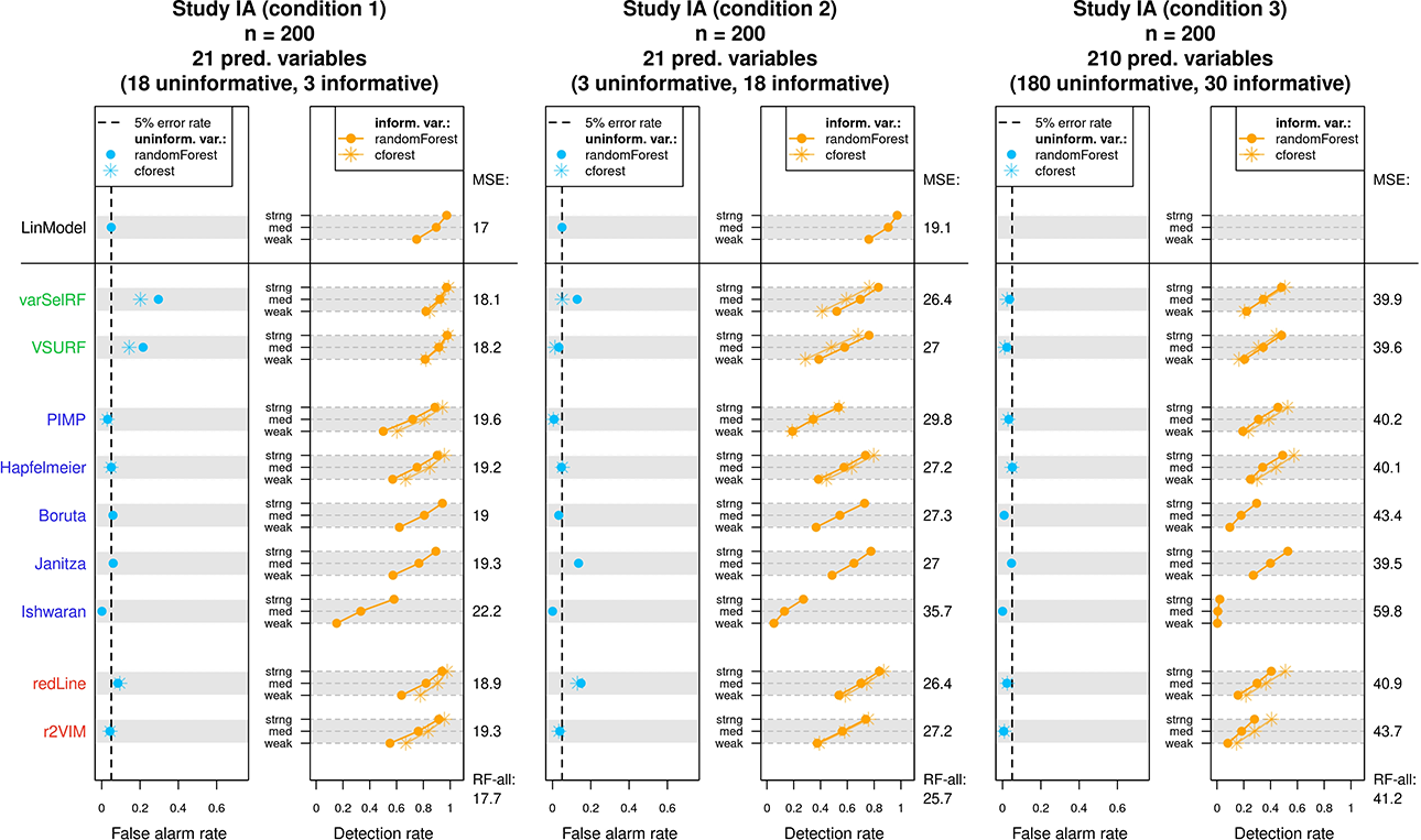
Results of Study IA. For each condition, the achieved mean false alarm and detection rates of the variable selection methods are displayed. The achieved mean squared errors on the test data are listed on the right side of each graph. See text for more details.

For all methods except Boruta, Janitza, and Ishwaran, Figure 4 additionally presents the results when using the cforest function instead of randomForest. These results are depicted with slightly transparent star symbols. Displayed above all methods are the results of the linear model (except in Condition 3, for which the linear model is not identifiable). Since the data generating process was based on the linear regression model, the results of the linear model represent near ideal performance. The predictive performances of the methods are displayed in Figure 4 as mean squared errors on the right-hand side for each condition. For comparison, the mean squared error is also indicated for a random forest that did not exclude any of the predictors (labeled as “RF-all”).

In the following examination of the results, we occasionally refer to specific properties of the individual methods. For a better understanding, we recommend to first inspect the detailed descriptions of the variable selection methods in the Online Supplementary Material.

The two performance-based methods (varSelRF and VSURF) showed the expected difficulty of adhering to a fixed false alarm rate. The achieved false alarm rates regularly surpassed the 5% mark, which partly explains the generally high detection rates. It seems that the two performance-based methods best adhered to a 5% false alarm rate in the third condition. In general, varSelRF showed higher false alarm rates than VSURF. This difference might be explained by the implemented “one-standard-error” rule in VSURF, which leads to a more restrained selection of variables. Further, the two performance-based methods showed relatively low test errors (indicated in Figure 4 on the right-hand side), a finding which is perhaps not further surprising since the two methods are designed to reach high prediction accuracy. In summary, these methods selected most informative predictors, but also several uninformative ones.

The five test-based methods (PIMP, Hapfelmeier, Boruta, Janitza, and Ishwaran) showed a slightly different pattern in their performance. In general, the test-based methods did not surpass the desired false alarm rate of 5%. The only exception was the Janitza method, which showed an increased false alarm rate in the second condition. Such a drop in the performance of the Janitza method in the second condition was not unexpected. Since the Janitza method relies on negative importance scores for variable selection, it was bound to struggle the most in a condition with few uninformative variables. In contrast, the methods PIMP, Boruta, and Ishwaran repeatedly fell below the 5% false alarm rate and, therefore, tended to be too conservative. This pattern was most accentuated in the Ishwaran method. The Ishwaran method showed an extremely low false alarm rate in all three conditions, which is also reflected in consistently low detection rates. Such a behavior suggests that the bootstrap estimator used in Ishwaran overestimated the variances of the importance scores in all conditions of Study IA. As a result, this method selected only few uninformative predictors, but also only few truly informative predictors. While PIMP and Boruta showed conservative false alarm rates as well, it was only Hapfelmeier, which successfully adhered to a 5% false alarm rate in all conditions. Regarding prediction accuracy, Janitza showed the lowest average test error rates of all test-based methods throughout the three conditions of Study IA, followed by Hapfelmeier.

Lastly, the remaining two “other” methods (redLine and r2VIM) showed a relatively mixed performance. r2VIM showed good performance in the first two conditions but exhibited too conservative variable selection in the third condition. Since the restrictiveness of r2VIM is directly dependent on the selection of its f parameter, it follows that the value of f was not chosen appropriately in the third condition. Tracking the selection of the f parameter throughout Study IA revealed that f was predominantly set to the minimal value of 0.5, which was still too large to achieve a false alarm rate of 5% in the third condition. ³ Thus, users might be interested in using a more extended search grid when tuning the f parameter, which comes at the cost of additional computational effort. The redLine depicted a pattern similar to the test-based method Janitza, showing an increased false alarm rate in the second condition, where there were only few uninformative variables, and the best performance in the third condition. Since the redLine, like Janitza, relies on negative importance scores for variable selection, the similarity between the two methods’ performance could be anticipated. In terms of prediction accuracy, the redLine showed the lower error rates of the two “other” methods.

As mentioned, Figure 4 also includes the results when the variable selection methods were run with the cforest function instead of the randomForest function (star symbols). For those methods where it was applicable, the cforest function led to slightly better performances in the majority of cases. This pattern is, for example, visible for the Hapfelmeier method, where using the cforest function led to higher detection rates without negatively affecting false alarm rates. Similar patterns can be observed for the methods PIMP, redLine, and r2VIM.

Figure 5 displays the collected computation times of the examined methods. The displayed boxplots represent the distribution of the recorded computation times for each method in each condition. Therefore, the median line in the boxplots gives an estimate of the expected duration when applying a specific variable selection method to a data set comparable in size to the one used in the specific condition. The method with the highest computation times in all conditions was the Hapfelmeier method, reaching computation times of over 24 hours in the third condition.

Figure 5.

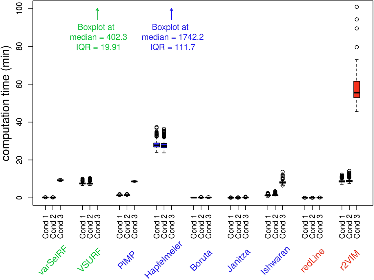
Computation times of variable selection methods in Study IA displayed as boxplots. Due to the high computation times, the boxplots of the methods Hapfelmeier and VSURF for condition 3 are not visible and only referred to by text.

In summary, the Hapfelmeier method stood out in Study IA as the variable selection method with the best statistical properties. Hapfelmeier was the only method which consistently adhered to a 5% false alarm rate, while maintaining comparatively high detection rates. The only disadvantage of the Hapfelmeier method was its high computation time. In cases where computation time is a limiting factor, possible alternatives are the test-based methods PIMP and Boruta.

Simulation Setting (Study IB)

Simulation Study IB followed the same general structure and simulation procedure as Study IA. Again, three conditions with varying numbers of informative and uninformative predictor variables (the same numbers as in Study IA) were simulated and the response variable was generated using a linear regression model. However, instead of combining three different effect sizes, Study IB combined three different variable types in each condition. Since psychological data commonly involve different types of variables (see, e.g., Aschwanden et al., 2020), the goal of Study IB was to inspect how this can affect the performance of the variable selection methods. The three simulated variable types included a continuous variable, a binary variable, and a nominally scaled variable with six categories. Equation 2 presents the regression equation for the first condition, which like in Study IA included three informative predictor variables (one of each type) and 18 uninformative predictor variables (six of each type). ⁴ The effect sizes of the three predictor types (b_c , b_b , and $b_{n_1}$ through $b_{n_6}$ ) stayed the same for all three conditions and were set in a way to achieve equal expected amounts of explained variance in the response variable by each predictor type (see the Online Supplementary Material for specific effect sizes). The goal of such an assignment was to give the same predictive value to each predictor type in order to prevent unwanted distortion of the variable selection process ⁵ :

$y_i=b_c{x}_{ci}+b_b{x}_{bi}+b_{n_1}{x}_{n_{1}i}+b_{n_2}{x}_{n_{2}i}+b_{n_3}{x}_{n_{3}i}+b_{n_4}{x}_{n_{4}i}+b_{n_5}{x}_{n_{5}i}+b_{n_6}{x}_{n_{6}i}+{\text{∊}}_i,$

2

with:

${\text{∊}}_i\stackrel{i\mathrm{.}i\mathrm{.}d}{\sim }\mathcal{N}(0,16),$

$x_c:\text{informative continuous variable,}$

$x_b:\text{informative binary variable,}$

$x_{n_1}\mathrm{,...},x_{n_6}:\text{informative nominally scaled variable}{\text{.}}^6$

Results (Study IB)

The results of Study IB are displayed in Figure 6. In general, Figure 6 follows the same structure as the presentation of results in Study IA, that is, for each condition and variable selection method, the achieved false alarm rates and detection rates are displayed. However, instead of different effect sizes, the three rows per method contain the results of the three different predictor types (denoted with “cnt” for continuous, “bin” for binary, and “nom” for nominally scaled predictors). Since the simulated data included uninformative variables of each predictor type, false alarm rates can be reported separately for each type (blue lines in left panels). Accordingly, the detection rates corresponding to informative variables of each predictor type are presented as orange lines in the right panels.

Figure 6.

Results of Study IB. For each condition, the achieved mean false alarm and detection rates of the variable selection methods are displayed. The achieved mean squared errors on the test data are listed on the right side of each graph. See text for more details.

In summary, the results of Study IB strongly echoed the results of Study IA. Therefore, reoccurring patterns such as elevated false alarm rates in performance-based methods or the tendency toward conservative variable selection in test-based methods are not again discussed. Looking at the individual selection methods in more detail reveals that performances did vary depending on the predictor type. For example, multiple selection methods exhibited a noticeable pattern in their achieved false alarm rates. These methods showed increased false alarm rates for the nominally scaled predictors with six categories and the continuous predictors compared to the binary predictors, resulting in many of the blue lines assuming the shape of a C in Figure 6. This behavior can be explained by the known properties of permutation importance scores in randomForest already shown by Strobl et al. (2007), in particular by the fact that the importance scores of variables with many cutpoints; in this case, the continuous and the nominally scaled predictors, show a larger variance. This allowed the continuous and the nominally scaled predictors to produce more high ranking importance scores compared to the binary predictors, which led to heightened false alarm rates in those methods whose selection strategy is directly based on the ranking of importance scores. In contrast, methods whose selection strategy incorporates a variance estimation of individual importance scores, such as, for example, PIMP, Hapfelmeier or Ishwaran, did not show the described distortion. Importantly, the results of the bias-free cforest function (star symbols) did not show the distortion either, independent of the used selection method.

Looking at the detection rates in the right panels of Figure 6 reveals a more diverse collection of patterns. In the top row, the linear model showed a decreased detection rate for nominally scaled predictors (the significance test for nominally scaled predictors was based on the F-statistic), which is not further surprising given the higher degrees of freedom associated with the nominally scaled predictor in the linear model. A similar pattern could be observed for some of the random forest-based approaches, such as, for example, the PIMP and Hapfelmeier method. In other methods, the abovementioned properties of randomForest importance scores were evident in the detection rates as well. In these cases, the detection rates indicated by the orange lines tended to assume the previously observed C-shape in favor of the continuous and the nominally scaled predictors, which is especially visible in the second and third conditions. Again, using the bias-free cforest function did not show a preference toward nominally scaled predictors and instead led to results more similar to the linear model’s performance.

When comparing the different methods throughout all three conditions, it was again the Hapfelmeier method, which stood out as the only method to abide by a false alarm rate of 5% while maintaining high detection rates. The computation times of Study IB (and all subsequent studies) are only reported in the Online Supplementary Material due to the similarity to previous results.

Study II

In the second simulation study, the variable selection methods were evaluated using more intricate data structures. The goal was to highlight some of the differences between variable selection using random forests and an analysis with a linear regression model. Study II comprised two substudies, Study IIA and Study IIB. In Study IIA, the artificial data newly included correlated predictors, which, as will become evident in the respective results, has profound effects on the variable selection process and the associated interpretation. Study IIB, on the other hand, focused on the presence of nonlinear effects and interactions between predictors. The simulation settings of Study IIA and Study IIB are described in the following.

Simulation Setting (Study IIA)

The artificial data in Study IIA followed the same general structure as in Study IA (Equation 1). The data consisted of 15 continuous predictor variables, of which six were uninformative variables and nine were informative variables. Like in Study IA, the informative variables were divided into three equally sized groups of weak, medium, and strong predictors. In contrast to Study IA, however, the predictor variables were not all sampled independently. The correlation structure was organized as follows: Three of the six uninformative variables were independently sampled. The other three uninformative variables were each correlated with one of the informative variables ( $r=0.7$ ), matching up one of the uninformative variables with a weak predictor, one with a medium predictor and one with a strong predictor. Three of the nine informative variables were accordingly each correlated with one of the uninformative variables. Three other informative variables (including one weak, medium, and strong predictor) were all correlated among each other ( $r=0.7$ ). Finally, the last three informative variables (including one weak, medium, and strong predictor) were independently sampled. The complete covariance matrix of the predictor variables is available in the Online Supplementary Material.

The reason for examining the effects of correlated predictors lies in a notable difference between variable importance scores in random forests and coefficients in linear regression models. The coefficients in a linear regression model express partial effects. Thus, the coefficient of a specific predictor informs about its relation with the response variable while taking into account the effects of all other predictors included in the model. As a simple example, one could imagine the relation of children’s reading ability with children’s age and children’s shoe size. One would expect that both age and shoe size do individually correlate with reading ability, that is, older children are more proficient in reading and children with larger feet are more proficient in reading. In this example, the relation between shoe size and reading ability is of spurious nature, driven by the connection between age and shoe size (older children wear larger shoes). Therefore, one can imagine that once the relation between age and reading ability is taken into account, shoe size does not provide additional information regarding a child’s reading ability. In this hypothetical scenario, a multiple linear regression, combining the two predictors age and shoe size, would detect a significant coefficient for age, but a coefficient around zero for shoe size (assuming linear relations between the variables). This characteristic of linear regression is commonly used to statistically control for potential confounder variables. In contrast, the permutation importance scores in random forests cannot be interpreted as an expression of partial effects (Debeer & Strobl, 2020; Strobl et al., 2008). Variables, which conditionally do not have a relation with the response variable (such as shoe size in the previous example), can still obtain a high importance score due to a correlation with a truly informative predictor (such as age in the previous example). The distinction in Study IIA between independent uninformative variables and uninformative variables which are correlated with informative variables intends to replicate exactly such a scenario and to show how the individual variable selection methods are affected by it. In addition, the permutation importance has been reported to generally favor correlated predictors (Nicodemus et al., 2010; Strobl et al., 2008). The distinction between independent and correlated informative variables aims at examining the behavior of the variable selection methods given such correlations.

Since permutation importance scores do not express partial effects, any variable selection approach based on permutation importance is expected to be affected to some degree by correlations between informative and uninformative predictors. However, there are proposals for alternative importance scores which aim at reflecting partial effects (Debeer & Strobl, 2020; Gazzola & Jeong, 2019; Strobl et al., 2008). These approaches follow the same general logic as the ordinary permutation importance, with the exception that the variable of interest is only permuted within specifically selected groups of observations to control for the influence of correlated variables. Thus, the importance score indicates the relation of the predictor with the response variable when correlated predictors are (nearly) held constant, which is intended to resemble the rationale of partial effects. Since the variable selection methods are (for the most part) not tied to a specific type of variable importance, an implementation using such a conditional permutation scheme is possible, as proposed in the context of causal inference by Keller (2019).

To investigate variable selection using a conditional permutation importance, Study IIA was extended with a second condition. The second condition followed the same data generating process as the first condition, but the variable selection methods were adapted to use the conditional variable importance proposed by Strobl et al. (2008), which is implemented in the R-package permimp (Debeer & Strobl, 2020). Since the transition to a conditional importance score was not feasible for the methods Ishwaran, Boruta, and Janitza, these methods were excluded from the second condition of Study IIA. In turn, the abovementioned Keller method (Keller, 2019) method was newly added. The Keller method, available in the R-package rfvarsel, essentially represents an application of the PIMP algorithm using a conditional permutation importance scheme implemented for forests fitted with the randomForest R-package. ⁷

In each condition of Study IIA, a data set consisting of 200 observations was simulated 1,000 times. The same outcomes as in Study I were examined for each selection method. In addition to reporting the results for randomForest and cforest, each with their default tuning parameter values, like in Study I, in the second condition of Study IIA we will display additional results for cforest, in which the trees were allowed to be more fully grown. ⁸ By means of this, we can illustrate that the effect of the conditional importance also depends on the tree depth, as shown in the subsequent results section.

Results (Study IIA)

The results of Study IIA are displayed in Figure 7. Similar to the presentation of the results in Study I, Figure 7 presents each condition in a separate graph. In contrast to Study I, however, false alarm rates and detection rates are separately reported for different classes of predictors.

Figure 7.

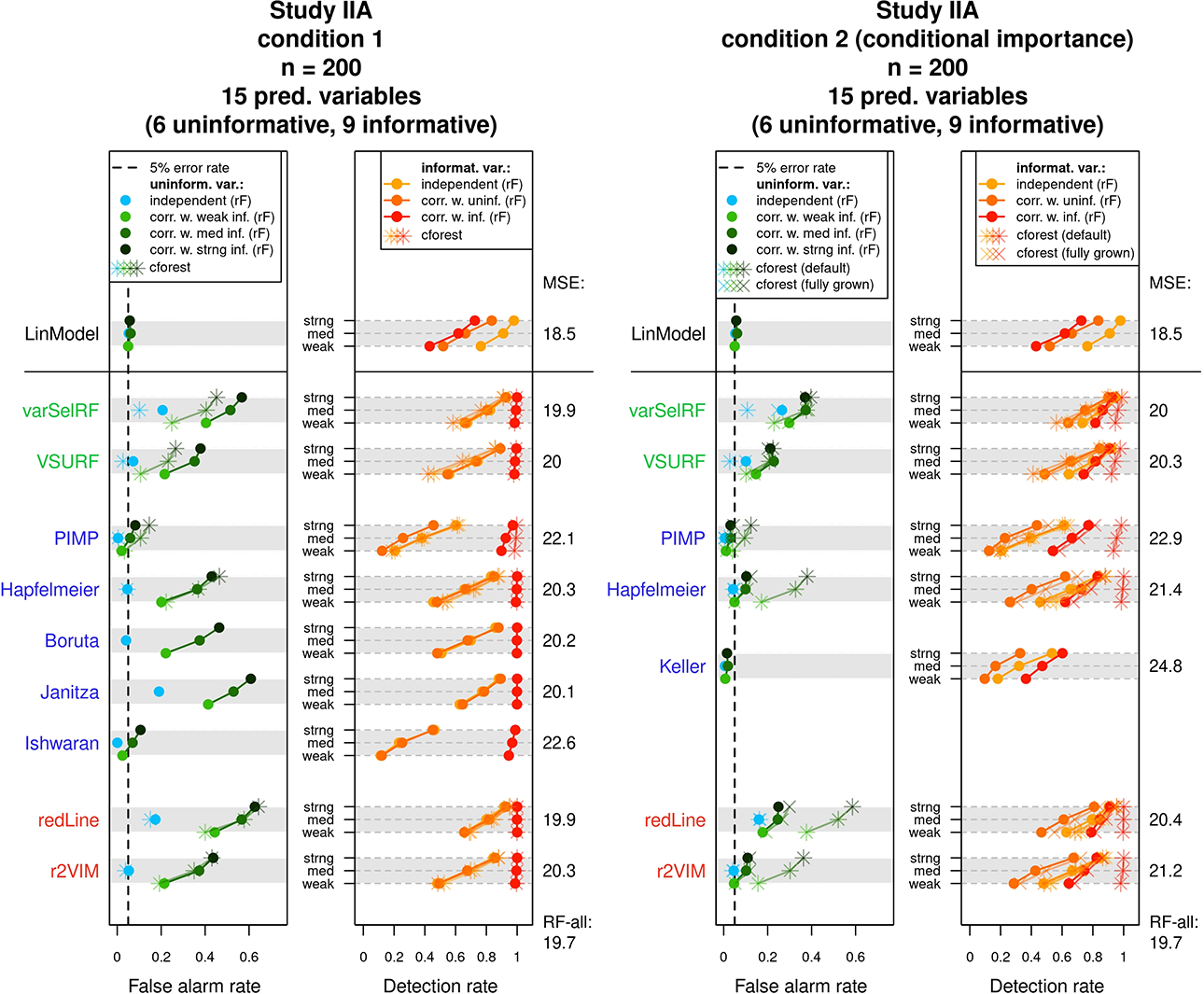
Results of Study IIA. For each condition, the mean false alarm and detection rates of the variable selection methods are displayed for different classes of variables. The achieved mean squared errors on the test data are listed on the right side of each graph. See text for more details.

In both conditions, the response variable was generated using a combination of independent and correlated linear predictors. As a result, false alarm rates (in the left panels) are separately reported for independent uninformative variables (light blue points) and uninformative variables which are correlated with informative variables (green points). Thus, the green points correspond to variables which themselves were not involved in the generation of the response variable (i.e., were uninformative) but were correlated with informative predictors. The three types of green points (light green, medium-dark green, and dark green) correspond to uninformative variables correlated with a weak, a medium, or a strong informative variable, respectively. The achieved detection rates (in the right panel of the graphs) are separately reported for three classes of predictors. These classes were independent informative variables (light orange points), informative variables that were correlated with uninformative variables (medium-dark orange points), and informative variables that were correlated with other informative variables (dark orange points). Again, the corresponding results when using the cforest function are indicated using star symbols. In the second condition, the additional results for the fully grown cforest are indicated using cross symbols.

The results in Condition 1 (left graph) exposed a pattern that highlights the described difference between random forest variable importance scores and a linear model’s variable coefficients. The linear model, whose coefficients express partial effects, adhered to a 5% false alarm rate for all types of uninformative variables. The random forest selection methods, however, showed a strong preference for the uninformative variables, which were correlated with informative predictors. As a result, the green points regularly surpassed the 5% false alarm rate. Exceptions were the PIMP and Ishwaran methods. The PIMP method, for example, showed a false alarm rate close to the desired 5% for correlated uninformative variables.

However, the abidance to the 5% rate in these cases was owed to a generally conservative selection behavior, which is recognizable by the very low false alarm rate for independent uninformative predictors and the generally low detection rates. Regarding the false alarm rates for independent uninformative variables (blue points), the methods Hapfelmeier, Boruta, and r2VIM have abided best to a rate of 5%.

In terms of detection rates, the results of the random forest methods differed again strongly from the pattern observed for the linear model. While the linear model showed the highest detection rate for independent linear predictors, the detection rate was slightly decreased for the correlated informative variables. The examined variable selection methods, however, tended to strongly prefer the informative variables, which were correlated among each other (dark orange points). Similar to the results of the false alarm rates, a correlation with an informative predictor increased the detection rate. On the other hand, the detection rates for light and medium-dark orange points were generally lower and tended to be equal. Thus, a correlation with an uninformative variable did not affect the detection rates of predictors. Apart from these specific preferences, the variable selection methods showed a similar pattern regarding the detection rates as in Study I. Of all methods which did not exceed the 5% false alarm rate (for independent uninformative variables), Boruta, r2VIM, and Hapfelmeier showed the highest detection rates.

The results changed in Study IIA’s second condition, where conditional importance scores were applied (the right graph of Figure 7). Since conditional importance scores intend to represent partial effects, the expectation was that the false alarm rates for correlated uninformative predictors (green points) would be brought down toward a rate of 5%. Such an effect was indeed observed and is especially well visible for the methods Hapfelmeier and r2VIM. Despite such a reduction in false alarm rates, the preference for correlated variables did not completely vanish. The correlated uninformative variables (green points) still tended to show higher selection rates than the independent uninformative variables (blue points) and also for the methods Hapfelmeier and r2VIM remained mostly above the 5% mark. What is particularly striking at first sight is that the effect of using conditional importance scores strongly differed between the randomForest and cforest function when using the respective default tuning parameter values. In contrast to the randomForest function, applying conditional importance scores with the cforest function using its default tuning parameter values only showed a minor reduction of false alarm rates. Since the computation of the conditional importance scores was identical for both types of forests, it is clear that the observed differences in the results must be due to differences in the structure of the generated forests. Indeed, it can be shown that the average tree depth is much larger for randomForest compared to cforest when using the default tuning parameter values. Deeper trees allow to account for more conditioning variables when calculating conditional importance scores. Accordingly, after adapting the tuning parameters of cforest to allow more fully grown trees, the resulting false alarm rates closely resembled those observed for randomforest. The results for the fully grown cforest are indicated using cross symbols in the right graph of Figure 7 and strongly overlap with the randomForest results.

The detection rates shown in the right panel of the graph were also affected by the conditional importance scores. In general, the use of conditional importance scores led to lower detection rates. The decrease in detection rates affected especially those informative variables which were correlated with other predictors, either other informative predictors (dark orange) or uninformative variables (medium-dark orange). As the cforest results show, the reduction of detection rates again depended on the tree depth, with the fully grown cforest showing decreased detection rates compared to its default implementation. The newly added Keller method showed a conservative selection behavior expressed by low false alarm and low detection rates. Therefore, it presented a similar pattern of results as the PIMP method, which is not further surprising given that Keller is based on the PIMP method.

In summary, none of the included methods in the second condition of Study IIA replicated the performance of the linear model, which may serve as an exemplar when the aim is to represent partial effects. Using conditional importance scores can help reduce the false alarm rates in the presence of correlated predictors, but the effect of conditioning also depends on other factors, in particular the tree depth. The false alarm rates still remained either too high (e.g., Hapfelmeier, r2VIM) or too conservative (PIMP, Keller). Which approach is most suited in a specific case may depend on the research question. For example, in cases where it is important not to include uninformative variables, the more conservative approaches might be preferred.

It should also be noted that the calculation of conditional importance scores is computationally more expensive compared to the conventional permutation importance. Thus, the computation times in the second condition of Study IIA were strongly increased (see Online Supplementary Material) and may for some methods approach unfeasible magnitudes especially given larger data sets than simulated in the present study.

Simulation Setting (Study IIB)

The generated data in Study IIB consisted of 24 predictor variables, of which six were uninformative variables and 18 were informative variables. The generation of the response variable y followed a slightly adapted linear model. In contrast to the previous simulations, the model now also included nonlinear effects and interactions between predictors. Specifically, the 18 informative predictors were divided into three classes of predictors. The first six informative variables were linear predictors, which exhibited linear effects on y. Similar to previous settings, the linear predictors were separated into three groups of equal size which exhibited weak, medium, and strong effects on the response variable. The next six informative variables were interacting predictors. The six interacting predictors formed three two-way interactions among each other, with each interaction term exhibiting a weak, medium, or strong effect on y. The last six informative variables were nonlinear predictors. The implemented nonlinear effects included a quadratic effect and a sine-shaped effect on y. Again, each type of effect was implemented with a weak, medium, and strong effect size. The described data pattern is presented in Equation 3, in which the three classes of predictors are shown on separated lines. As visible in Equation 3, the interaction and some of the nonlinear effects were increased by a factor of three. Additionally, the sample size was increased to 400. These adjustments were performed to facilitate the detection of the included complex effects in order to prevent floor effects in the methods’ achieved detection rates:

$\begin{array}{l}{y}_i=b_w(x_{1i}+x_{2i})+b_m(x_{3i}+x_{4i})+b_s(x_{5i}+x_{6i})\\ +b_w(3x_{7i}{x}_{8i})+b_m(3x_{9i}{x}_{10i})+b_s(3x_{11i}{x}_{12i})\\ +b_w(x_{13i}^2+3sin(x_{14i}))+b_m(x_{15i}^2+3sin(x_{16i}))+b_s(x_{17i}^2+3sin(x_{18i}))\\ +{\text{∊}}_i,\end{array}$

3

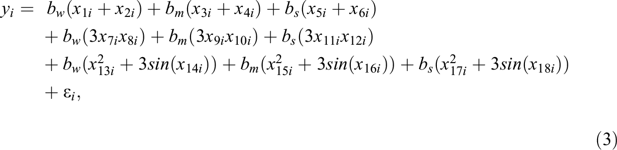
with:

${\text{∊}}_i\stackrel{i\mathrm{.}i\mathrm{.}d}{\sim }\mathcal{N}(0,16),$

$x_1\mathrm{,...},x_6:\text{linear predictors,}$

$x_7\mathrm{,...},x_{12}:\text{interacting predictors,}$

$x_{13}\mathrm{,...},x_{18}:\text{nonlinear predictors,}$

$b_w=0.8,b_m=1,\text{and}{b}_s=\mathrm{1.2.}$

Nonlinear and interaction effects can be present in empirical data and may pose difficulties for an analysis using a linear model. Although a linear regression model would be perfectly capable of modeling the simulated data structure if the nonlinear and interaction terms were correctly specified, in practice, the presence and exact form of nonlinear effects or interactions is not known a priori and has to be discovered through explorative analyses or theoretical considerations. In lack of previous knowledge of such effects, researchers often apply a naive linear model, in which all predictors are assumed to only exhibit a linear main effect on the response variable. Variable selection with a random forest is supposed to offer an advantage in such a scenario since the random forest has the ability to autonomously detect complex patterns in the data. Such patterns would also be reflected in the variables’ importance scores and be taken into account in the variable selection process. Therefore, Study IIB intends to illustrate a scenario, in which a random forest can achieve a better performance than a naive linear model.

Study IIB followed the same general simulation procedure as Study IIA. Unlike in the previous simulations, however, not the true linear model but a naive linear model, which only assumes linear main effects for each predictor, was evaluated for comparison.

Results (Study IIB)

The results of Study IIB are presented in Figure 8. The recorded false alarm rates were similar to the results for independent uninformative variables observed in Study IIA and are not further discussed. The detection rates in the right panel are reported for the three different classes of variables. These classes were informative variables with a linear main effect (light orange), informative variables with an interaction effect (medium-dark orange), and informative variables with a nonlinear effect (dark orange). The implemented interaction effects and nonlinear effects hampered detection with a naive linear model, which assumed only linear main effects for each predictor. This is reflected in the detection rates observed for the naive linear model in the top row. Both the variables with nonlinear effects and the variables with only interaction effects showed very low selection rates compared to the variables with linear main effects. In contrast, the random forest selection methods were able to detect the influences of these variables, which is recognizable by the generally higher detection rates for the medium-dark and dark orange points. In general, the methods, which showed the highest detection rates, given that the false alarm rate of 5% was not exceeded, were again the Hapfelmeier method and the r2VIM method.

Figure 8.

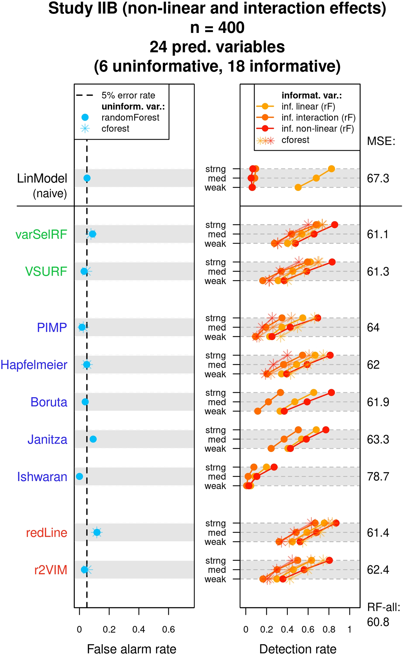
Results of Study IIB. The mean false alarm and detection rates of the variable selection methods are displayed for different classes of variables. The achieved mean squared errors on the test data are listed on the right side of each graph. See text for more details.

Inspecting the test errors collected in Study II revealed a similar pattern as in Study I, with the two performance-based methods varSelRF and VSURF showing the lowest test errors on average.

Discussion

The present investigation aimed at providing an introduction to the concept of variable selection with random forests and to examine the statistical properties of various variable selection methods. Although the underlying data structures were of simple nature, Simulation Study I already revealed marked differences between the selection methods. In general, the examined methods tended to either not control the false alarm rate or to exhibit too conservative variable selection. Interestingly, the study revealed one exception, which was the Hapfelmeier method. As the only method which consistently adhered to the targeted false alarm rate of 5% while retaining relatively high detection rates, Hapfelmeier showed the best performance throughout Study I.

The second simulation study slightly differed in its goals from the first study. By examining the detection of correlated predictors, nonlinear effects, and interaction effects, the study intended to highlight differences between an analysis with random forests and a conventional linear modeling approach. The demonstrated differences in Study II were two-fold. First, Study IIA showed how variable selection with random forests cannot generally be interpreted as an expression of partial effects. Second, Study IIB showed how random forests are able to autonomously detect informative predictors with nonlinear or interaction effects. Importantly, these two properties are mostly linked to the nature of random forest variable importances in general and not to the variable selection procedures themselves. Therefore, the observed properties do not necessarily help in distinguishing the performances of the individual selection procedures, since almost all of them are affected in a similar fashion. The results rather serve as an instructional example regarding the use and interpretation of random forests. Especially, the results of Study IIA come with important practical implications. Since the original permutation importance does not express partial relationships like the coefficients in a linear model, one cannot interpret the permutation importance as being detached from the other predictors’ influence. Therefore, using the original permutation importance in variable selection with random forests, it is not possible to control for confounders by including them as predictors (as is commonly done in linear modeling).

The representation of partial effects can to some degree be improved by using conditional importance scores. However, as shown in the results of Study IIA, the effectiveness of conditioning remains ambiguous and depends on other factors, in particular on tree depth. With fully grown trees, the conditioning showed to be more effective in this study, but the general effect of tree depth on random forest performance and interpretation should be further investigated in future research. It is also important to note that whether the inability to detect partial effects is perceived as a disadvantage depends on the goals and research questions of the investigator. There are lines of investigation where the aim is to identify any predictor which relates to the response variable, as, for example, in certain genetic screening studies (Goldstein et al., 2011). When the shape of the relation between response variable and predictors is unclear, random forests have the additional benefit of flexibly detecting nonlinear and higher order effects (as shown in Study IIB). One natural exploitation of this trait is the application of random forests in exploratory analyses. Similar to genetic screening studies, random forests could help researchers in the social sciences to find previously unknown relations between variables of interest. In practice, variable selection with random forests could, for example, be performed as an addition to parametric analyses with linear or generalized linear models. If a random forest-based method identifies additional variables that the linear models did not identify, this might be due to undetected nonlinear or interaction effects. In a reversed fashion, random forests could also be used to preselect a subset of predictors to be included in a following analysis. However, note that statistical inference performed on the same data after model selection is no longer valid without appropriate correction (Berk et al., 2013; Fithian et al., 2014). This problem can be avoided by using new data for the final model.

Apart from the two demonstrated differences between random forest variable selection and a conventional linear model analysis, Study II showed a similar pattern for the examined selection methods as Study I. Again, the Hapfelmeier method showed comparatively good performance regarding the false alarm rates and detection rates. Importantly, the good performance of Hapfelmeier was not only observed in the presented regression setting but also extended to the setting of classification (see Online Supplementary Material). The success of the Hapfelmeier method throughout the present study only partly relates to the results of previous comparison studies (see Table 1). The only study which recommended the Hapfelmeier method was Hapfelmeier and Ulm (2013). Other studies predominantly recommended the Boruta method and no special mentioning of Hapfelmeier is to be found, even in those studies that included it. While Boruta also performed well in our simulations, compared to Hapfelmeier, it showed a stronger tendency to deviate from the targeted false alarm rate. The discrepancy in the results is possibly due to the type of evaluation in the respective studies. Both other studies which included the Hapfelmeier method focused exclusively on predictive performance and not on selection rates. Accordingly, there were methods in our study, including Boruta, which slightly outperformed Hapfelmeier in terms of test errors. However, the results regarding predictive performance should be treated with caution. Predictive performance is directly related to the amount of retained informative variables. Therefore, the most inclusive variable selection methods tended to achieve the lowest test errors (at the expense of heightened false alarm rates). This point is illustrated by the fact that a random forest without any variable selection (i.e., keeping all predictors, indicated in the result figures as RF-all) generally achieved the lowest test errors throughout our studies. ⁹ Also, it should again be noted that when the goal of a study is to identify relevant predictors, for example, in order to decide which variables to include in a subsequent investigation, then the false alarm rate and detection rate of a variable selection method are more important evaluation criteria than the achieved prediction accuracy.

Given the wide variety of results presented here, it is difficult to come up with general and concise recommendations for empirical researchers. Rather than advocating the use of one specific technique, we primarily want to urge researchers to be conscious of the characteristics and peculiarities of the presented methods, especially with regard to the differences from the interpretation of linear model coefficients. We hope that the reader of the present work can conceive an informed opinion about whether variable selection with random forests can be of use to them. If variable selection is performed, we recommend to use the Hapfelmeier method. Depending on the research question and the structure of the data, combining the Hapfelmeier method with a conditional importance measure can help to account for partial effects of predictors. Relative to the other examined methods, Hapfelmeier’s performance was only inferior in terms of the required computation time. Although the computation time of Hapfelmeier can be long and perhaps unfeasible when working with very large data sets, for common psychological data sets, the associated time requirements seem justifiable. In cases where the computation time is a major obstacle, we recommend the Boruta or PIMP method.

Although variable importance scores and the associated variable selection help interpret the role of predictors, random forests do retain some of their black-box qualities. Apart from variable importance scores, there are other techniques which aim at facilitating the interpretation of random forests. Such methods, for example, include the use of partial dependence plots to describe the shape of a predictor’s relation with the response variable (Henninger et al., 2023). Further investigations of different interpretation methods and possible combinations thereof might allow more insights into random forests in the future and help make their application more accessible to social scientists.

Supplemental Material

Supplemental Material, sj-pdf-1-jeb-10.3102_10769986231193327 - Identifying Informative Predictor Variables With Random Forests

Supplemental Material, sj-pdf-1-jeb-10.3102_10769986231193327 for Identifying Informative Predictor Variables With Random Forests by Yannick Rothacher and Carolin Strobl in Journal of Educational and Behavioral Statistics