Sage Journals: Discover world-class research

Abstract

A general framework of latent trait item response models for continuous responses is given. In contrast to classical test theory (CTT) models, which traditionally distinguish between true scores and error scores, the responses are clearly linked to latent traits. It is shown that CTT models can be derived as special cases, but the model class is much wider. It provides, in particular, appropriate modeling of responses that are restricted in some way, for example, if responses are positive or are restricted to an interval. Restrictions of this sort are easily incorporated in the modeling framework. Restriction to an interval is typically ignored in common models yielding inappropriate models, for example, when modeling Likert-type data. The model also extends common response time models, which can be treated as special cases. The properties of the model class are derived and the role of the total score is investigated, which leads to a modified total score. Several applications illustrate the use of the model including an example, in which covariates that may modify the response are taken into account.

Keywords

thresholds model latent trait models item response theory classical test theory

1. Introduction

The development of item response theory (IRT) that clearly separates the observed response from the underlying latent traits has been mainly driven by the consideration of binary items, in which it is distinguished between a correct response and an incorrect one as outlined, for example, in Rasch (1960). Items with continuous response formats have been largely considered within the framework of classical test theory (CTT), which distinguishes between a true score, essentially the expected response, and an error score (Lord & Novick, 2008). Although there are some approaches to modeling continuous responses, there seems no general framework available that considers responses as generated by latent traits and item characteristics.

Continuous responses occur in particular in the form of time to complete a task and responses within a line segment (e.g., responses on a visual analogue scale). Especially, time response modeling, which has already been considered by Rasch (1960), has drawn much attention (De Boeck & Wilson, 2004; Ferrando & Lorenzo-Seva, 2007; Roskam, 1997; van der Linden, 2006). Also, Likert-type scales, which are quite common in practice, are often modeled as continuous responses despite of an ongoing discussion as to whether that is the right way to analyze this type of data. An overview concerning problems and the pros and cons have been given by Harpe (2015). The controversy focuses on the problem as to whether Likert-type categories constitute interval-level measurement or have to be treated as ordered responses. If the measurement level is only ordinal, then it is questionable if item sums should be used. Harpe (2015) distinguishes between the “ordinalist” and the “intervalist” view and concludes that “individual rating items with numerical response formats at least five categories in length may generally be treated as continuous data.” Although one has not to agree, it seems worthwhile to investigate whether there is much difference between continuous and discrete modeling, given proper latent trait models for both cases are available. One particular case which exemplifies these considerations is given by fitting normal theory-based models with robust standard errors to categorical factor analysis (FA) models (Rhemtulla et al., 2012). Although a practically feasible approach, the standard errors may become biased; however, depending on the sample size and number of categories, the effect may diminish.

When modeling responses that are restricted in some way, it is sensible to account for restrictions in a proper way. Otherwise, the models do not match the data. For illustration, let us consider an example in which data are confined to the interval $[1, 7]$ . If one uses normal distribution models, the restriction is simply ignored. Figure 1 shows the resulting distributions for the self-regulation data set to be considered in detail later if one assumes the latent trait model considered here but with varying assumptions concerning the distribution of responses. The first row shows the fitted distributions if one assumes that responses follow a normal distribution in a model that is equivalent to a unidimensional FA model. The left side shows the distributions for a medium value of the person parameter, and the right side shows the distributions for a high value of the person parameter. It is seen that the model does not yield proper distributions since the support of the distributions is not confined to the interval $[1, 7]$ . The same happens if one assumes a log-normal distribution (second row). Again, the upper boundary is totally ignored. The third row shows the fits for a continuous latent trait model that explicitly accounts for the fact that responses are restricted to the interval $[1, 7]$ . It is seen that the resulting distribution is much more adequate. The pictures show the problems with the upper boundaries, which in this application are more serious. Since observations were between 1.6 and 7 and the means of responses were 5.264 (Item 1), 5.643 (Item 2), and 5.492 (Item 3), the problems with the lower bounds would occur only for extremely small values of the person abilities.

Figure 1.

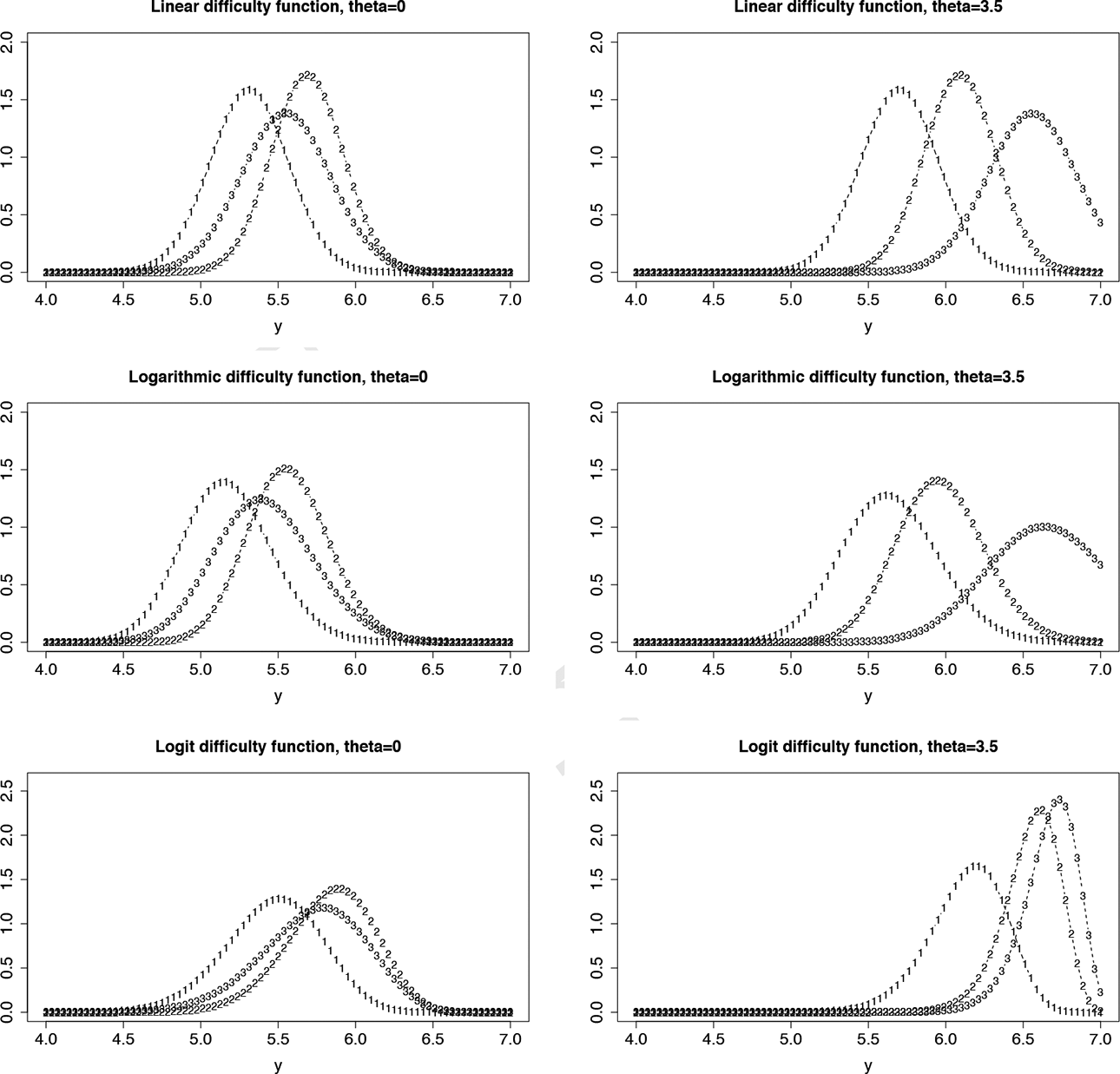
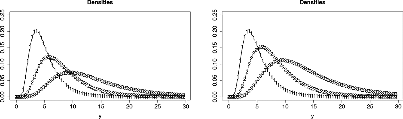
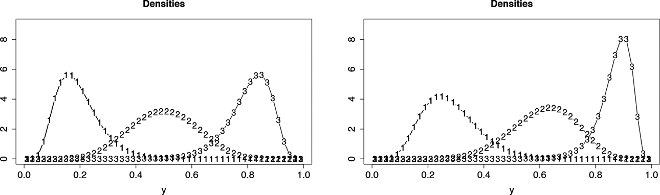
Estimated densities for self-regulation. First row: linear difficulty functions, second row: logarithmic difficulty functions, third row: logit difficulty functions, left: $θ_{low} = 0$ , and right: $θ_{high} = 3.5$ .

The objective of the present article is to propagate genuine latent trait models for continuous responses and investigate their properties. The general framework that is used is the thresholds model framework (Tutz, 2022b). The threshold model has been proposed as a model that allows for different item formats, but continuous responses have been treated very cursorily. In the following, the focus is on continuous responses and the approach is extended in several ways. The link to various versions of the CTT model is investigated in detail, basic results are obtained by using quantile functions, which have not been considered before, and the role of total scores is examined and modified versions are proposed. Also, the embedding of response time models, the comparison of models with differing response functions, and the explicit inclusion of explanatory variables have not been investigated before. Further, referring to the potential use in a Likert-type scale setting, we emphasize the need to properly account for the support of the data and show how this can be accomplished via the general modeling framework.

The general framework for continuous item response models does not only include various models as special cases but offers new modeling strategies that allow for valid inference. For responses that are restricted to an interval, as in analogue scales, one obtains models that account for the restriction. The models yield better fits and, importantly, yield more trustworthy significance tests, which is in particular helpful if the impact of covariate effects is to be investigated. Significance test based on the assumption of a normal distribution, which implies that responses can take values far beyond the fixed interval of responses, cannot be considered as reliable if responses are restricted. Problems with significance tests may occur any time if the distribution is strongly misspecified. Thus, alternative distributions are useful beyond the improvement of fits that can be obtained. For responses in the positive domain, the framework offers alternative distributions beyond the log-normal distributions and more flexible parameterizations.

This article is structured as follows: In Section 2, the general modeling framework is presented. In Section 3, we discuss linear models and show that the model allows for a variety of response distributions. Also, the link to CTT is investigated in detail. It is shown how the CTT model can be given as a genuine latent trait model. It also covers CTT-type models with alternative response distributions. Although the basic CTT model lacks distributional assumptions, some distributional assumptions are often tacitly assumed when fitting unidimensional CTT models via FA. Interesting distributions of practical relevance are in particular obtained when using nonlinear thresholds models (Section 4). The models allow one to find distributions that account for the restriction to closed or open intervals, yielding models that are much more appropriate than distribution models that ignore these restriction as, for example, the normal distribution. Section 5 is devoted to transformed responses and the link to thresholds models is investigated. In Section 6, the modeling approach is illustrated by using several data sets with differing response formats. It includes an example with reaction time data and shows how better fitting models than classical response time models can be constructed. Within the application section, Likert-type data are also discussed. It is shown that if one uses continuous modeling of Likert-type items, which is not uncommon, one should at least account for the fact that responses are restricted to an interval; otherwise, models show distinctly inferior fit.

2. Thresholds Models: Basic Concepts

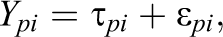
Let $Y_{p i}, p = 1, \dots, P, i = 1, \dots, I,$ denote the responses of person p on item i having support S_i . As is common in IRT, we assume local stochastic independence between the responses on different items given $θ_{p}$ . The general threshold model (Tutz, 2022b) is given by

P (Y_{p i} > y | θ_{p}, α_{i}, δ_{i} (.)) = F (α_{i} (θ_{p} - δ_{i} (y))),

where $F (.)$ is a strictly monotonically increasing, fixed distribution function, $θ_{p}$ is a person parameter, $α_{i}$ is a strictly positive discrimination parameter, and $δ_{i} (.)$ is a nondecreasing item-specific function, called item difficulty function, which is defined on the support S_i . The function $F (.)$ is a response function, which in combination with the difficulty function determines the distribution of the response. The form of the model reminds of binary response models as the normal-ogive or the two parameter logistic model, which are indeed special cases if one considers discrete responses $Y_{p i} \in {0, 1}$ and defines the item difficulty parameter by $δ_{i} = δ_{i} (0)$ (and additionally setting $δ_{i} (1) = \infty$ ). However, in the present article, we confine ourselves to metric responses.

One of the important features of the model is that $F (.)$ is a strictly increasing distribution function. Therefore, for fixed threshold y, the probability of a response larger than y increases with increasing person parameter $θ_{p}$ , which makes the model a sensible latent trait model—fulfilling the properties of a monotone homogeneity model (Sijtsma & Molenaar, 2002) and thereby allowing nonparametric tests of the implied conditional association assumption (Holland & Rosenbaum, 1986). The parameter $θ_{p}$ can be seen as an ability or attitude parameter, which indicates the tendency of a person to obtain a high score. Higher values of $θ_{p}$ are associated with a greater chance of scoring above some threshold y for each item. When using convenient marginal estimation methods, one has to assume a distribution for the person parameters, for details, see Tutz (2022b).

The concrete form of the thresholds model is determined by the choice of the difficulty functions ${δ_{i} (.)}_{i = 1, \dots, I}$ and the response function F. The model can be abbreviated by TM(F, ${δ_{i} (.)}$ ). If all the $δ$ -functions have the same structure, we will use a different notation instead of explicitly giving the functions. For example, if $F (.)$ is the (standard) normal distribution function and the difficulty is linear, that is, of the form $δ_{i} (y) = δ_{0 i} + δ_{i} y$ , then we will abbreviate this as TM(normal, linear).

3. Linear Models

We will first consider models in which the mean of the response is a linear function of the latent ability. This can be obtained within the framework of thresholds models by assuming that the difficulty functions are linear. An important feature is that any strictly continuous response distribution can be obtained by combining a linear difficulty function with a response function that is chosen according to the assumed response.

3.1. Linking Latent Traits and Responses

Let $F (.)$ denote a fixed, typically standardized, distribution function with support $ℝ$ , for example, the standardized normal distribution function, and $f (y) = \partial F (y) / \partial y$ be the corresponding density. In addition, let the difficulty function be linear, $δ_{i} (y) = δ_{0 i} + δ_{i} y$ , $δ_{i} > 0$ . Thus, we are considering threshold models of the type TM(F, linear).

When investigating the distribution of responses, it is helpful to define the distribution function $\bar{F} (y) = 1 - F (- y)$ . If a random variable Y has distribution function $F (.)$ , the random variable $- Y$ has distribution function $\bar{F} (.)$ . With $\bar{f} (y) = \partial \bar{F} (y) / \partial y$ denoting the density corresponding to $\bar{F} (.)$ , one obtains for the distribution and the density of responses

F_{p i} (y) = P (Y_{p i} \leq y) = 1 - F (α_{i} (θ_{p} - δ_{0 i} - δ_{i} y)) = \bar{F} (α_{i} (δ_{0 i} + δ_{i} y - θ_{p})),

f_{p i} (y) = \partial F_{p i} (y) / \partial y = f (α_{i} (θ_{p} - δ_{0 i} - δ_{i} y)) α_{i} δ_{i} = \bar{f} (α_{i} (δ_{0 i} + δ_{i} y - θ_{p})) α_{i} δ_{i} .

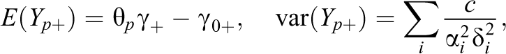
That means the distribution function of the responses, $F_{p i} (y)$ , is a shifted and scaled version of $\bar{F} (.)$ , with the shifting and scaling depending on the person and the item.

The expectation and variance of $Y_{p i}$ have the form (Proposition 8.4 in the Appendix)

μ_{p i} = E (Y_{p i}) = \frac{θ_{p} - δ_{0 i} - μ_{F} / α_{i}}{δ_{i}} = γ_{i} θ_{p} - γ_{0 i},

σ_{p i}^{2} = var (Y_{p i}) = \frac{{var}_{F}}{α_{i}^{2} δ_{i}^{2}},

where $γ_{i} = 1 / δ_{i}$ , $γ_{0 i} = (δ_{0 i} + μ_{F} / α_{i}) / δ_{i}$ , and $μ_{F}, {var}_{F}$ are constants that are determined by the distribution function $F (.)$ . More concretely, $μ_{F} = \int y f (y) d y$ is the expectation corresponding to distribution function $F (.)$ , and ${var}_{F} = σ_{F}^{2} = \int {(y - E_{F})}^{2} f (y) d y$ is the corresponding variance. The main point is that the responses have a distribution function, which is a shifted and scaled version of $\bar{F} (.)$ , the means are linear functions of $θ_{p}$ , and the variances depend only on the items. For symmetric distribution $F (.)$ , one simply has $F (.) = \bar{F} (.)$ and $μ_{F} = 0$ . Then, responses follow the distribution function $F (.)$ .

It is noteworthy that one can choose any fixed function $F (.)$ (or $\bar{F} (.)$ ) and obtain a model, in which responses follow the distribution function $\bar{F} (.)$ simply by using a linear difficulty function. In particular, one is not restricted to normal distribution models, as is often done in applied research but can try alternative distributions including nonsymmetric ones. If, for example, one assumes for $\bar{F} (.)$ the Gumbel distribution, also known as maximum value distribution, $\bar{F} (y) = exp (- exp (- y))$ , one obtains for the responses a Gompertz distribution, $G (y) = 1 - exp (- exp (y))$ , and if one assumes the Gompertz (or minimum value) distribution, one obtains for the responses the Gumbel distribution.

For illustration, Figure 2 shows the distributions obtained for a person with $θ = 0$ . The first row shows the densities if a normal distribution is assumed, the second row shows the densities if $F (.)$ is the standardized Gumbel distribution. The left picture shows the results for three items with parameters $(2, 1), (0, 1), and (- 2, 1)$ (for $(δ_{0 i}, δ_{i})$ ); in the right picture, the slopes are varying with parameters $(2, 0.8), (0, 1), and (- 2, 1.2)$ . In all the pictures, $α_{i} = 1$ . If slopes are equal (left picture), the intercepts determine the difficulty of the item, and the highest responses are to be expected for Item 3, which has the smallest intercept ( $δ_{0 i}$ ). If slopes vary across items, the mean and the variance change. Item 3 has the smallest variance since it has the highest slope (right picture). The second row shows the corresponding densities if a Gompertz distribution is assumed for $F (.)$ ; consequently, the responses follow the (skewed) Gumbel distribution.

Figure 2.

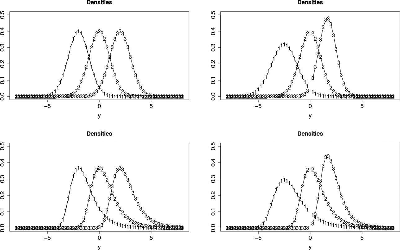
Densities for three items with equal slopes and varying intercepts (first column) and for three items with varying slopes (second column). First row: normal response function; second row: Gumbel for $\bar{F} (.)$ .

The derived results hold for all strictly continuous distribution functions $F (.)$ , not only for functions with support $ℝ$ . Note, however, that for distribution functions with a smaller support, the support of the item scores typically differs for different latent abilities. If a response function with only positive support is chosen, that is, if $F (x) = 0$ holds for $x < 0$ , then for fixed y, one may always find a large enough negative $θ$ , such that $(θ - δ (y)) < 0$ , and hence, $P (Y_{p i} > y) = 0$ holds for that value of y. Whether this poses a practical problem depends on the probability distribution of the latent variable. Such a dependency of the support on $θ$ is avoided if one restricts to response functions, which are positive throughout $ℝ$ (as in the case of a normal or Gumbel distribution).

3.2. Thresholds Models and CTT

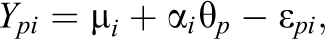
In CTT, the response usually is decomposed into the “true score” and the “error score,” typically at the population level. A similar decomposition holds for threshold models on the population level and the person level. At the person level, one has

Y_{p i} = τ_{p i} + ε_{p i},

where the noise variable $ε_{p i}$ has expectation $E (ε_{p i}) = 0$ and variance $var (ε_{p i}) = {var}_{F} / (α_{i}^{2} δ_{i}^{2})$ (the full derivation is given in Proposition 8.1 in the Appendix). Moreover, the true score $τ_{p i}$ equals the expected value of $Y_{p i}$ , and it depends on p only via $θ_{p}$ , that is, two test takers with the same latent ability possess the same true score.

One can then define—following Novick (1966) and Holland and Hoskens (2003)—the true score random variable T_i as the true score of a randomly selected test taker from the population and the error variable $ε_{i}$ as the correspondingly sampled noise variable, when testing the selected test taker. That is, on the random sampling level, wherein Y_i denotes the response of a randomly selected test taker on the ith item, the following equation holds

Y_{i} = T_{i} + ε_{i} .

Herein, $T_{i} = T_{i} (θ) : = E (Y_{i} | θ)$ and $ε_{i} = ε_{i} (θ) : = Y_{i} - T_{i} (θ)$ are the functions of the random variable $θ$ . All central axioms of the CTT model (Novick, 1966) are implied by the properties of a general (not necessarily linear) TM model—as shown in Proposition 8.1 in the Appendix. Basically, these axioms boil down to the existence of an additive decomposition (6) for each item, with the additional properties that (i) errors on different items are uncorrelated, (ii) errors and true scores are uncorrelated, and (iii) the expectation of the error given the true score is zero.

This representation has several consequences. Given that a threshold model holds a CTT model holds for randomly selected test takers. Thus, all CTT based quantities, like reliability coefficient, may be defined appropriately, and all of the derived results for true score prediction may be applied to the TM setting (for details, we refer to Holland and Hoskens (2003)). Hence, a plethora of already established results become applicable. Another important aspect is that the threshold model can be seen as a latent trait model underlying the CTT model. In the CTT model, expectations of item responses are simply considered as representing the true scores, but latent traits as the driving force behind the individual’s responses on items are not clearly identified. We note, however, that the unrestricted CTT model is in almost any cases fulfilled by appropriate definitions of the true and error score terms (Novick, 1966). It only imposes empirical testable restrictions when it is used in its restricted form—via submodels (which are further described in the following). These submodels are oftentimes estimated via the factor analytical approach—hence, in practical applications of CTT models, there is a close connection to normal theory-based FA models—despite the fact that the original CTT setup lacks any distributional assumptions.

Now, assuming the special case of a linear TM model, one may derive specific submodels of CTT. To this end, it is helpful to recall the following distinction (Raykov, 1997): Measurements are called congeneric if all true scores may be expressed as affine functions of a single true score, that is, $T_{i} = a_{i} T + b_{i}$ holds for some fixed values $a_{i} and b_{i}$ . This equals the notion of unidimensionality from a CTT point of view (providing also the decomposition of the covariance matrix according to a one-dimensional FA model, albeit lacking the independence assumptions). This property is always satisfied for a linear TM (see Equation 7), but not necessarily for a general TM. For the linear model, one obtains from (3)

T_{i} (θ) = E (Y_{i} | θ) = \frac{θ - δ_{0 i} - μ_{F} / α_{i}}{δ_{i}},

and therefore

θ = δ_{i} T_{i} (θ) + δ_{0 i} + μ_{F} / α_{i} .

Thus, measurements are congeneric. As will be shown in the following, in nonlinear TMs, $θ$ is a nonlinear function, and measurements are not congeneric. It should be noted that the two notions of unidimensionality (IRT vs. CTT) do not coincide. A TM model may be classified as a unidimensional IRT model according to common definitions (Holland & Rosenbaum, 1986), but if it is not a linear TM model, then the corresponding CTT model is not necessarily unidimensional (in the sense used in CTT modeling).

The latter is caused solely by the fact that the CTT-based definition of unidimensionality requires linear relationships on the level of the true scores, whereas a general TM model provides a nonlinear relation, as the following argument shows. The dependency of the ith true score on $θ$ is represented by $T_{i} (θ) = E (Y_{i} | θ)$ . One may now fix some item i (without loss of generality $i = 1$ ) and express the latent ability as a function of the true score T on that item via $θ(T) = T_{1}^{- 1} (T)$ , where T denotes the true score on the first item (note that T ₁ denotes the function, whereas T is used to denote the true score variable). Substituting this expression for $θ$ , the true score on any other item can be expressed as a function of the true score of the reference item: $T_{j} (T) : = T_{j} (θ (T))$ . In general, these functions differ from linearity, and hence, one does not arrive at a congeneric CTT model.

One may further subdivide the congeneric model—assuming in the following a linear TM. Measurements are called essentially tau-equivalent if $a_{i} = 1$ holds for all i in the congeneric relationships $T_{i} = a_{i} T + b_{i}$ (or upon redefinition of T, we may just demand $a_{i} = c$ for some constant c). As is seen from (7), the model is congeneric model with $a_{i} = 1 / δ_{i}$ and $b_{i} = - (μ_{F} α_{i}^{- 1} + δ_{i,0}) / δ_{i}$ . This congeneric model is essentially tau-equivalent if $δ_{i} = 1$ holds for all i. Two important consequences of tau-equivalency shall be pointed out: First, conditionally on $θ$ , the expected value of the unweighted mean of the item scores equals the latent variable plus a bias value (determined by the intercept term). As the bias term is independent of $θ$ , one may deduce that the difference of means of two test takers provides an unbiased estimate of their true difference in the ability—thus justifying the usage of simple sum scores (although there are statistically more efficient estimators). Second, commonly applied coefficients—such as Cronbach’s α—become reasonable estimators of the test reliability when tau-equivalency can be assumed (Jackson & Agunwamba, 1977).

The even stricter requirement of essentially parallel measurements demands in addition to tau-equivalency the equality of the error variances. From Equation 4, one obtains

Var (ε_{i}) = Var (E (ε_{i} | θ)) + E (Var (ε_{i} | θ)) = E (Var (Y_{i} | θ)) = \frac{{var}_{F}}{α_{i}^{2} δ_{i}^{2}} .

Accordingly, if $δ_{i} = 1$ (which is necessary and sufficient for essentially tau-equivalency) holds, all the error variances will be equal only if the discrimination parameters are also equal.

Two consequences of parallelity are worth mentioning. First, the best linear predictor of the true score weighs all item scores equally, providing further justification for the usage of simple sum scores. Second, the estimation of test reliability via the split-half approach is justified.

Taken together, these results show that

(1) on the second-order level (i.e., using only conditional expectations and variances), the general threshold model yields CTT models, and

(2) the unidimensional CTT model can be motivated by an underlying linear threshold model.

3.3. Quantile Function and Further Properties

It has already been highlighted that the mean is a linear function of the latent ability and that the variance does not depend on $θ$ , but one may go further and examine the dependency of quantiles and quantile-based measures of spread on the latent ability.

The quantile function for the response $Y_{p i}$ and values $0 < q < 1$ is given by

Q_{Y_{p i}} (q) = inf {y | 1 - F (α_{i} (θ_{p} - δ_{i} (y))) \geq q} = inf {y | δ_{i} (y) \geq θ_{p} - F^{- 1} (1 - q) / α_{i}} .

For strictly increasing difficulty functions $δ (\cdot)$ mapping onto $ℝ$ , which are assumed in the following, it has the simpler form

Q_{Y_{p i}} (q) = δ_{i}^{- 1} (θ_{p} - F^{- 1} (1 - q) / α_{i}) .

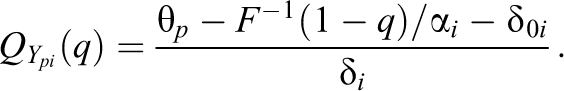
We now examine the case of linear difficulty functions more closely. Since difficulty functions are linear, one obtains $δ_{i}^{- 1} (x) = (x - δ_{0 i}) / δ_{i}$ , and the quantile function reduces to

Q_{Y_{p i}} (q) = \frac{θ_{p} - F^{- 1} (1 - q) / α_{i} - δ_{0 i}}{δ_{i}} .

Therefore, each quantile of $Y_{p i}$ is a linear function of $θ_{p}$ . For any $q \in (0, 1)$ , the q-quantile increases linearly with $θ_{p}$ . A further consequence of the form of the quantile function is that common measures of spread that are based on quantiles, for example, the interquartile range $Q_{Y_{p i}} (.75) - Q_{Y_{p i}} (.25)$ , do not depend on $θ_{p}$ .

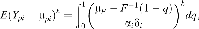
The quantile function may be used to derive formulas for the moments of $Y_{p i}$ . For the central moments, one obtains

E {(Y_{p i} - μ_{p i})}^{k} = \int_{0}^{1} {(\frac{μ_{F} - F^{- 1} (1 - q)}{α_{i} δ_{i}})}^{k} d q,

see Proposition 8.4. A consequence is that also central moments do not depend on $θ_{p}$ . It underlines that the person parameter just shifts the distribution of responses but does not affect its form, which is determined by the item parameters only.

A simpler form of the density of responses may be obtained by rewriting (2) in centered form as

f_{p i} (y) = \bar{f} (α_{i} (δ_{0 i} + δ_{i} y - θ_{p})) α_{i} δ_{i} = \bar{f} (α_{i} δ_{i} (y - \frac{θ_{p} - δ_{0 i}}{δ_{i}})) α_{i} δ_{i} .

From the change of variable formula, one may deduce from Equation 10 the following:

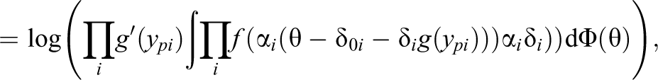
Let X denotes a random variable with distribution function $\bar{F}$ . Then, the random variable $Y : = a X + b$ with $a : = \frac{1}{α_{i} δ_{i}}$ and $b : = \frac{θ_{p} - δ_{0 i}}{δ_{i}}$ is distributed as $F_{p i}$ .

A common measure for the performance of persons that is typically used is the total score $Y_{p +} = \sum_{i} Y_{p i}$ . In linear models, the expectation and variance are given by

E (Y_{p +}) = θ_{p} γ_{+} - γ_{0 +}, var (Y_{p +}) = \sum_{i} \frac{c}{α_{i}^{2} δ_{i}^{2}},

where $γ_{+} = \sum_{i} γ_{i}$ , $γ_{0 +} = \sum_{i} γ_{0 i}$ . Thus, for linear threshold models, the expected total score is essentially the latent score, and the variance does not depend on $θ_{p}$ .

4. Nonlinear Models

In traditional item response models like the Rasch model or the normal-ogive model, the mean response is a nonlinear function of the person’s latent trait. This is sensible because the means in binary responses are restricted to the interval [0,1] and linear functions tend to take values outside this interval. In general, nonlinear functions are always to be expected if the response is restricted in some way. This holds also if responses are continuous but restricted, for example, to take positive values only, which is the case in many applications.

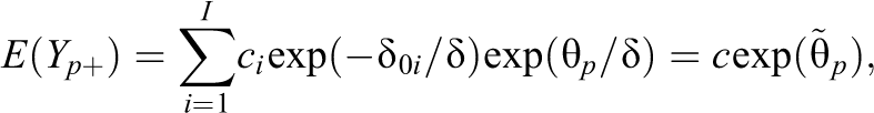
Within the framework of threshold models, restrictions on the support of responses are obtained in a natural way by specifying appropriate nonlinear difficulty functions. This leads to models, in which the mean and other characteristics of the responses are the nonlinear functions of the latent trait. In the following, we consider difficulty functions of the form $δ_{i} (y) = δ_{0 i} + δ_{i} g (y)$ , where $g (.)$ is a strictly increasing fixed function.

4.1. Responses in the Positive Domain

Let the response function $F (.)$ be chosen as fixed. The threshold model automatically restricts the responses to positive values, if for the difficulty function ${lim}_{y \to 0} δ_{i} (y) = - \infty$ holds. One candidate, which will be considered in more detail, is the logarithmic function $g (y) = log (y)$ , yielding $δ_{i} (y) = δ_{0 i} + δ_{i} log (y)$ .

For illustration, Figure 3 shows the response distributions for three items if the difficulty function is the logarithmic function. The left picture shows the distribution if the response function is the normal distribution; on the right side, the Gompertz distribution has been used as a response function.

Figure 3.

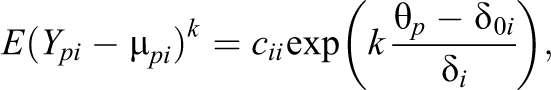
Densities for three items, logarithmic difficulty functions. Left: normal response function with intercepts and slopes given by $(- 3, 2), (- 4, 2), and (- 5, 2)$ , and right: Gumbel for $\bar{F} (.)$ with intercepts and slopes given by $(- 3, 2), (- 4, 2.5), and (- 5, 3)$ .

Expectations and variances of responses are no longer linear functions of the person parameter. For the logarithmic function, one obtains

E (Y_{p i}) = c_{i} exp (\frac{θ_{p} - δ_{0 i}}{δ_{i}}),

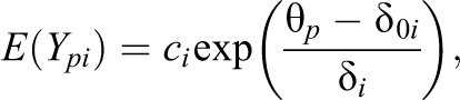
where c_i is a constant that depends on $α_{i} {and δ}_{i}$ (Proposition 8.4). Thus, expectations are exponential functions of the latent ability. The same holds for the central moments

E {(Y_{p i} - μ_{p i})}^{k} = c_{i i} exp (k \frac{θ_{p} - δ_{0 i}}{δ_{i}}),

where $c_{i i}$ is again a constant that depends on $α_{i} {and δ}_{i}$ (Proposition 8.4) and for the quantile function, which has the form

Q_{Y_{p i}} (q) = exp ((θ_{p} - F^{- 1} (1 - q) / α_{i} - δ_{0 i}) / δ_{i}) .

4.1.1. Decomposition

One can again try to decompose into a true score and an error score by using the representation

Y_{p i} = τ_{p i} + ε_{p i},

where $τ_{p i} = E (Y_{p i})$ and $ε_{p i}$ is implicitly defined by $ε_{p i} = Y_{p i} - τ_{p i}$ . However, the decomposition is quite different from the decomposition for linear difficulties in (5) since now the distribution of the error score depends on $θ_{p}$ . Even the support of $ε_{p i}$ depends on $θ_{p}$ since $ε_{p i} \geq - τ_{p i}$ .

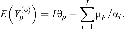
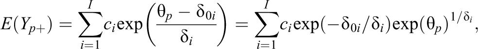
The form of the expectation has the consequence that the total score $Y_{p +} = \sum_{i} Y_{p i}$ , which is often used to measure the ability, is not appropriate. One has

E (Y_{p +}) = \sum_{i = 1}^{I} c_{i} exp (\frac{θ_{p} - δ_{0 i}}{δ_{i}}) = \sum_{i = 1}^{I} c_{i} exp (- δ_{0 i} / δ_{i}) exp {(θ_{p})}^{1 / δ_{i}},

which is a weighted sum of exponential terms with the terms depending on the item (Proposition 8.4). Conditions under which the total score is an appropriate measure have been investigated in particular for categorical responses (see, e.g., Hemker et al., 1997; Hemker et al., 2001; Masters, 1982; Sijtsma & Hemker, 2000). In the present case, a condition is that items are homogeneous, that is, $δ_{i} = δ_{i}$ for all i. In this case, one obtains

E (Y_{p +}) = \sum_{i = 1}^{I} c_{i} exp (- δ_{0 i} / δ) exp (θ_{p} / δ) = c exp ({\tilde{θ}}_{p}),

where ${\tilde{θ}}_{p} = θ_{p} / δ$ is the scaled ability and $c = \sum_{i} c_{i} exp (- δ_{0 i} / δ)$ . Thus, in the homogeneous case, $E (Y_{p +})$ is an exponential function of the scaled ability ${\tilde{θ}}_{p}$ . Of course, one can also consider the transformed ability $exp ({\tilde{θ}}_{p})$ as a measure of ability. Then, $E (Y_{p +})$ depends linearly on the (transformed) ability. Thus, in the homogeneous case, but only then, the total score can be considered as representing the underlying ability. Moreover, it holds only if the difficulty function is logarithmic.

4.1.2. Link to classical response-time models

If one assumes for $F (.)$ the standard normal distribution and a logarithmic difficulty function, the density of responses becomes

f_{p i} (y) = f (α_{i} (δ_{0 i} + δ_{i} log (y) - θ_{p})) α_{i} δ_{i} / y,

= (\sqrt{2 π})^{- 1} exp (- {(α_{i} (δ_{0 i} + δ_{i} log (y) - θ_{p}))}^{2} / 2) α_{i} δ_{i} / y,

= \frac{1}{y \sqrt{2 π} {\bar{σ}}_{i}} exp (- \frac{{(log (y) - {\bar{μ}}_{p i})}^{2}}{2 {\bar{σ}}_{i}^{2}}),

where ${\bar{μ}}_{p i} = (θ_{p} - δ_{0 i}) / δ_{i}$ and ${\bar{σ}}_{i} = 1 / (α_{i} δ_{i})$ . This is the lognormal distribution with parameters ${\bar{μ}}_{p i} {and \bar{σ}}_{i}$ . The homogeneous version of the model ( $δ_{i} = δ$ ) is equivalent to van der Linden’s lognormal response-time model, which is a speed model that carefully distinguishes between time and speed (van der Linden, 2016).

The threshold version of van der Linden’s model is a generalization allowing for varying slope parameters. It also offers the possibility to consider alternative response functions that replace the normal distribution and might yield better fit (see the application in Section 6.2).

4.2. Responses in an Interval

Let again the response function $F (.)$ be chosen as fixed. If responses are known to be restricted to the interval $(a, b)$ , then for the difficulty function, ${lim}_{y \to a} δ_{i} (y) = - \infty$ and ${lim}_{y \to b} δ_{i} (y) = \infty$ should hold. A candidate is the logit function $g (y) = log ((y - a) / (b - y))$ , yielding $δ_{i} (y) = δ_{0 i} + δ_{i} log ((y - a) / (b - y))$ . For simplicity, one can also transform the data into the interval $(0, 1)$ and use the simpler function $g (y) = log (y / (1 - y))$ .

For illustration, Figure 4 shows the distributions that are obtained for the interval $(0, 1)$ and standard normal distribution $F (.)$ . The underlying item parameters are $(3, 2), (0, 2), and (- 3, 2)$ (for $(δ_{0 i}, δ_{i})$ ). The left picture shows the distribution of responses if $θ_{p} = 0$ ; in the right picture, $θ_{p} = 1$ . It is seen that responses are within the interval $(0, 1)$ . For larger values of $θ_{p}$ , the distribution is not just shifted but distinctly changes its form.

Figure 4.

Distributions of responses for items with intercept and slope given by $(3, 2), (0, 2), and (- 3, 2)$ with logit difficulty function. Left: $θ = 0$ and right: $θ = 1$ .

Similar pictures are obtained if other difficulty functions that restrict the responses to an interval are used. To this end, all inverse distribution functions can be used. For simplicity, we focus on the logit function, that is, the inverse logistic distribution, which in the applications section is shown to outperform difficulty functions that ignore the restriction.

For the expectation and variances of responses, one obtains rather complicated formulae, which are not given. As in the case of logarithmic difficulty functions, they depend on the person’s ability $θ_{p}$ . Also, the simple total score depends on the ability in a complex form and cannot be considered an appropriate measure of the underlying latent trait. However, one can use the transformed total score considered in the next section, which typically is quite different from the conventional total score.

The case of responses in intervals is especially important in Likert-type items, which by definition are restricted to a fixed interval $[1, m]$ in m-grade Likert-type scales. As already shown in Figure 1, ignoring the restriction to an interval yields improper densities, which typically are positive beyond the interval $[1, m]$ . In addition, the total score as a sum of responses over items is not a reliable indicator of the latent trait.

5. Transformation of Responses and Linearity

It is interesting that at the heart of all threshold models, there is a linear relationship between abilities and expectations; however, it does not relate to the expectations of the responses itself but to transformed responses. More concise, one can derive the general result

E (δ_{i} (Y_{p i})) = θ_{p} - μ_{F} / α_{i}, var (δ_{i} (Y_{p i})) = {var}_{F} / (α_{i} δ_{i})^{2},

where $μ_{F} and {var}_{F}$ are again the expectation and variance corresponding to distribution function $F (.)$ (Proposition 8.6). It means, in particular, that the expectations of transformed responses are linear functions of the person parameter; in the case of $α_{i} = 1$ , additionally, the intercept of the linear function does not depend on the item.

One can establish a simple general relationship between the TM and the chosen response function $F (.)$ , if the difficulty function is fixed. It can be shown (see Proposition 8.5 in the Appendix) that

δ (Y_{p i}) has the same distribution as θ - Y_{0} / α_{i},

where Y ₀ follows the distribution function $F (.)$ Hence, on the level of the transformed variable, the latent ability $θ$ acts as a simple location parameter, thereby shifting expectations and quantiles in a linear manner, as already described previously.

One consequence of (11) is that the expected transformed total score $Y_{p +}^{(δ)} = \sum_{i} δ_{i} (Y_{p i})$ is a linear function of the ability

E (Y_{p +}^{(δ)}) = I θ_{p} - \sum_{i = 1}^{I} μ_{F} / α_{i} .

Thus, $Y_{p +}^{(δ)}$ can be seen as an indicator of the ability, for example, $\frac{(Y_{p +}^{(δ)} - Y_{q +}^{(δ)})}{I}$ provides an unbiased estimator of $θ_{p} - θ_{q}$ . With $δ_{i} (y) : = δ_{0 i} + δ_{i} g (y)$ and $δ_{0} = \sum_{i = 1}^{I} δ_{0 i}$ , it has the form

Y_{p +}^{(δ)} = δ_{0} + \sum_{i = 1}^{I} δ_{i} g (Y_{p i}),

which is a weighted sum of transformed responses.

The previous considerations suggest that one could also work with the transformed responses $g (Y_{p i})$ and formulate models for the transformed responses. Let us consider the thresholds model with strictly increasing transformation $g (.)$ mapping onto $ℝ$ , TM(F, { $δ_{0 i} + δ_{i} g (y)}$ ), which is given by

P (Y_{p i} > y | θ_{p}, α_{i}, δ_{i} (.)) = F (α_{i} (θ_{p} - δ_{0 i} - δ_{i} g (y))) .

If the model holds, one obtains for the transformed responses $g (Y_{p i})$

P (g (Y_{p i}) > z | θ_{p}, α_{i}, δ_{i} (.)) = P (Y_{p i} > g^{- 1} (z) | θ_{p}, α_{i}, δ_{i} (.)) = F (α_{i} (θ_{p} - δ_{0 i} - δ_{i} z)),

which means that $g (Y_{p i})$ follows the linear threshold model TM(F, linear) with the same item parameters. Thus, fitting of TM(F, { $δ_{0 i} + δ_{i} g (y)}$ ) for observations $Y_{p i}$ and fitting of TM(F, linear) for observations $g (Y_{p i})$ yield the same parameters.

When comparing models with different specifications as, for example, different difficulty functions, one can use goodness-of-fit measures as the log-likelihood or Akaike information criterion (AIC) values of the models. However, some caution is warranted if transformed data are considered. Although the TM(F, { $δ_{0 i} + δ_{i} g (y)}$ ) for the original data and the TM(F, linear) for the transformed data yield the same parameters, log-likelihood or AIC values should not be compared.

The log-likelihood contribution of observation ${(Y_{p i})}_{i = 1, \dots I}$ when fitting TM(F, { $δ_{0 i} + δ_{i} g (y)}$ ) via marginal maximum likelihood (MML) is

l_{p} = log (\int (\prod_{i} f (α_{i} (θ - δ_{0 i} - δ_{i} g (y_{p i}))) α_{i} δ_{i}) g^{'} (y_{p i})) d Φ (θ)),

= log (\prod_{i} g^{'} (y_{p i}) \int \prod_{i} f (α_{i} (θ - δ_{0 i} - δ_{i} g (y_{p i}))) α_{i} δ_{i})) d Φ (θ)),

= \sum_{i} log (g^{'} (y_{p i})) + log (\int \prod_{i} f (α_{i} (θ - δ_{0 i} - δ_{i} g (y_{p i}))) d Φ (θ)) .

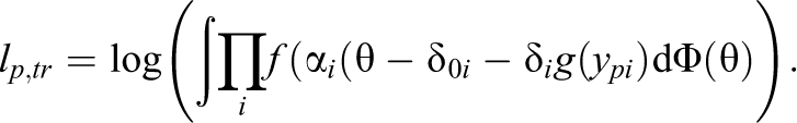
The log-likelihood contribution of the transformed observation $g {(Y_{p i})}_{i = 1, \dots I}$ when fitting TM(F, linear) is

l_{p, t r} = log (\int \prod_{i} f (α_{i} (θ - δ_{0 i} - δ_{i} g (y_{p i}) d Φ (θ)) .

Since the term $log (g^{'} (y_{p i}))$ does not contain the parameters, the maximization of the likelihood $l = \sum_{p} l_{p}$ yields the same parameters as maximization of the likelihood $l_{t r} = \sum_{p} l_{p, t r}$ . However, the likelihoods l and $l_{t r}$ have differing values and comparing them would be misleading.

A consequence is that the choice of difficulty functions should not be based on comparing fits of transformed data. Response transformations $g_{1} (Y_{p i})$ and $g_{2} (Y_{p i})$ and the corresponding fits of a linear thresholds model refer to different data. In contrast, fitting of thresholds models by using the original data but differing difficulty functions yields likelihoods that indicate which model shows better fit to the data.

As an example, we use the self-regulation data to be considered later (Section 6.1). The log-likelihood obtained when fitting a model with normal response function and logarithmic difficulty function is −654.136, and when fitting a model with linear difficulty function to the log-transformed data, one obtains −326.531. These models should definitely not be compared via goodness-of-fit measures based on their log-likelihoods although parameter estimates for both models are identical.

6. Applications

We illustrate the usage of the nonlinear TM models with three examples. Along with the modeling of properly continuous data, like response times, we will in particular focus on the practical usage of the application of these models to Likert-type scales, whereby in contrast to a direct linear, unrestricted treatment, we take care of the range of the restricted support via appropriately chosen difficulty functions.

All models are fitted using the MML-procedure and Gauss–Hermite quadrature, whereby a centered normal distribution with unknown variance $σ_{θ}^{2}$ for the latent variable is specified and wherein identifiability issues are resolved by fixing the item discrimination parameter on the first item to unity. The full R-Code is provided as Supplementary Material. We abstain from including the likelihood and score functions, which can be found in Tutz (2022b).

6.1. Self-Regulation

The data set Lakes from the R package MPsychoR (Mair, 2018) is a multifacet G-theory application taken from Lakes and Hoyt (2009). The authors used the response to assess children’s self-regulation in response to a physically challenging situation. The scale consists of three domains: cognitive, affective/motivational, and physical. We use the physical domain only. Each of the 194 children was rated by five raters on three items on their self-regulatory ability with ratings on a scale from 1 to 7. We use the average rating over the five raters, which yields a response that takes values in the interval $(1, 7)$ but is not confined to integer values.

Table 1 shows log-likelihoods and estimates of $σ_{θ}$ for various responses and difficulty functions with varying slopes in the difficulty functions. The columns on the left show fits for fixed discrimination parameters ( $α_{i} = 1$ ), and the right columns show fits for varying discrimination parameters. In addition, the likelihood ratio tests that compare the fits of varying discrimination parameters models and fixed discrimination parameters models are given. It is seen that varying discrimination parameters yield significantly better fits. For example, the likelihood ratio test that compares the fixed discrimination model and the varying discrimination model is 21.090 on 2 df for the Gumbel model with logit difficulty function. Similar results hold for the other models. For given response function F, the best fits are always obtained via logit difficulty functions. Conversely, for a given difficulty function, the best fit is obtained by choosing the Gumbel distribution as response function F. Consequently, the best fit is found if the response function is the Gumbel function and the difficulty function is the logit function, and the corresponding fits are indicated by an asterisk.

Table 1.

Fits for Self-Regulation Data

		$α_{i} = 1$		$α_{i}$ Varying
Response fct	Difficulty fct	Log-lik	${\hat{σ}}_{θ_{p}}$	Log-lik	${\hat{σ}}_{θ_{p}}$	Likrat
Normal	linear	−563.084	1.493	−554.421	2.596	17.326
	log	−654.136	1.260	−644.621	2.379	19.030
	logit	−521.785	1.729	−515.111	2.264	13.348
Logistic	linear	−542.951	2.753	−531.891	4.404	22.120
	log	−594.417	2.507	−561.602	6.370	65.630
	logit	−509.584	3.179	−500.133	4.324	18.902
Gumbel	linear	−525.132	1.758	−514.559	2.643	21.149
	log	−552.629	1.584	−549.302	2.607	6.654
	logit	−508.218*	1.989	−497.673*	2.948	21.090
Gompertz	linear	−597.118	1.837	−594.366	1.955	5.504
	log	−694.613	2.174	−684.997	2.818	19.232
	logit	−550.887	1.939	−542.893	2.384	15.988

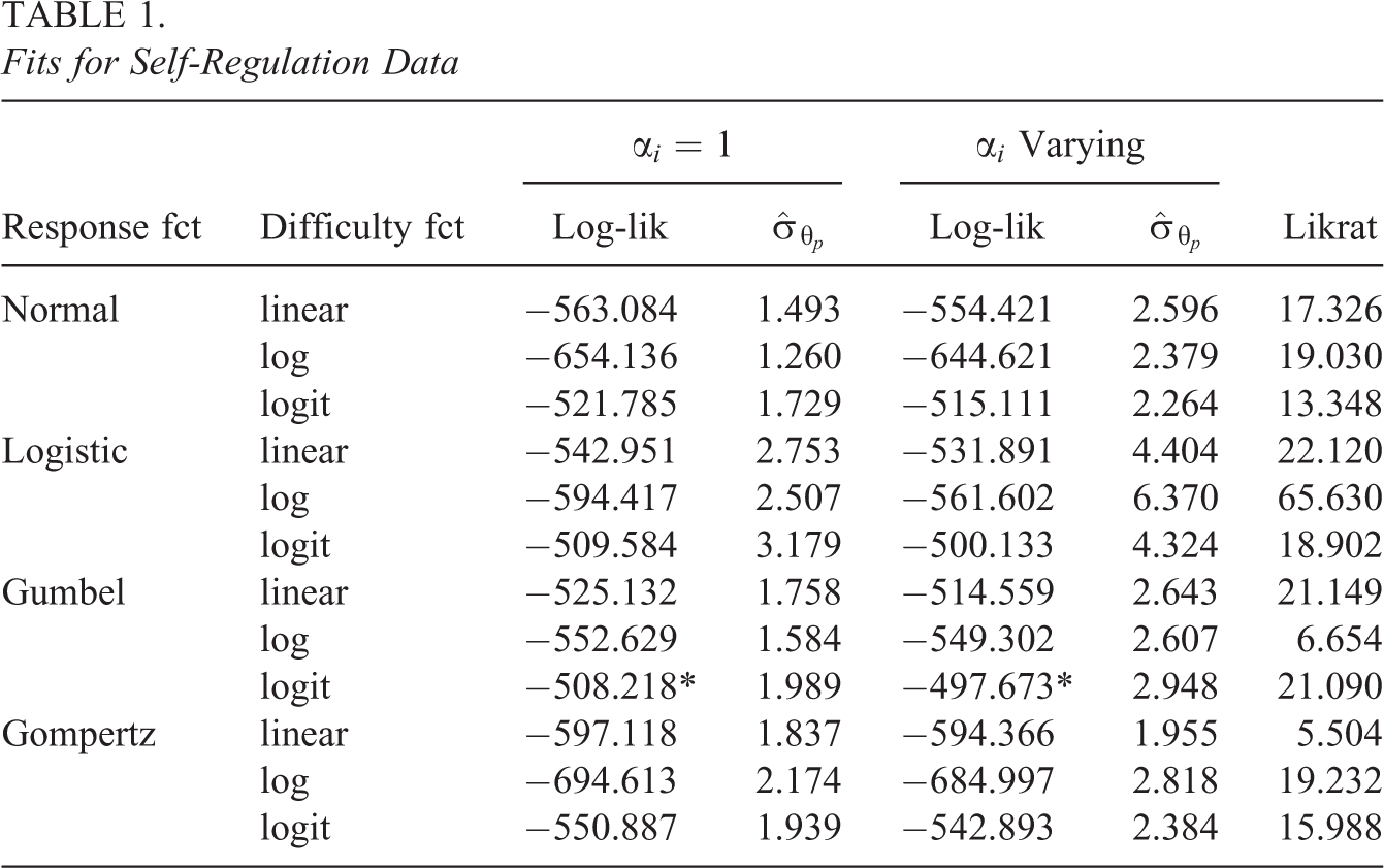
The example demonstrates that better fits are obtained when the restriction of the responses to a fixed interval is taken seriously by using logit difficulty functions. Although a skewed response function as the Gumbel function performs better when using inadequate difficulty functions as the linear function, there is not much support for preferring the Gumbel response function over the symmetric logistic function. The corresponding log-likelihoods (−497.673 and −500.133) are very close.

Figure 1, which has already been considered in Section 1, shows the estimated response densities for the three items with varying discrimination parameters (using as response function the normal distribution). First row shows linear difficulty functions, second row shows logarithmic difficulty functions, third row shows logit difficulty functions, left column shows responses for latent trait $θ_{low} = 0$ , and right column shows responses for latent trait $θ_{high} = 3.5$ , which is not extreme given ${\hat{σ}}_{θ_{p}}$ is larger than 2.5. It is seen that linear and logistic difficulty functions yield inappropriate densities that take values outside the interval $(1, 7)$ . The logit difficulty function, which restricts the responses, yields much more appropriate distributions.

To demonstrate the consequences of fitting models that ignore the restrictions on the support of responses, the posterior estimates of person parameters have been computed for the model with a normal response function and linear difficulty function (varying discrimination parameters). Figure 5 shows the predicted distributions for Item 3 that are obtained for the 20 largest estimated person parameters. It is seen that for many of them, the mode is above the threshold 7. If modes were used as estimates of the performance on the item, one would obtain values that are beyond the threshold. It demonstrates that predictions on tasks similar to Item 3 are bound to yield improper values.

Figure 5.

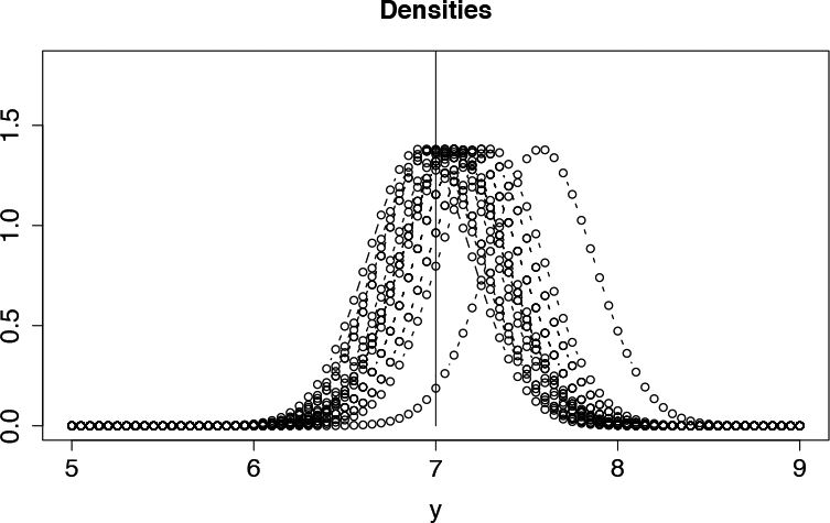
Densities of Item 3 evaluated at the 20 largest values of estimated person parameters when using the TM with a normal response function and linear difficulty function.

6.2. Rotation Response Time

The R package diffIRT contains response time data of 121 subjects to 10 mental rotation items. Each item consists of a graphical display of two three-dimensional objects. The second object was either a rotated version of the first object or a rotated version of a different object. Subjects were asked whether the second object was the same as the first object (yes/no). The degree of rotation of the second object was 50°, 100°, or 150°. Response times were recorded in seconds.

We fitted thresholds model with logarithmic difficulty function and fixed discrimination parameter. The best fit was obtained for the normal response function (loglik −1,300.378, $σ_{θ} = 0.817$ ), which outperformed the Gumbel response function (loglik −1,390.093) and the Gompertz response function (loglik −1,321.674). Testing if slopes in the difficulty functions can be modeled as constant yields the likelihood ratio statistic 32.486 on 9 df, which indicates that slopes should be considered as varying across items (see also Table 2). As already mentioned in Section 4.1, the homogeneous model with slopes that do not vary across items is equivalent to the lognormal model proposed by van der Linden (2016; assuming normal response function and logarithmic difficulty functions). In this application, the model seems inadequate since the nonhomogeneous model yields significantly better fit to the data.

Table 2.

Parameter Estimates for Response Time Data With Varying and Constant Slopes

	Varying Slopes		Common Slopes
Item	Intercept	Slope	Intercept	Slope
[1]	−3.132322	3.196110	−2.873841	2.950614
[2]	−1.866113	2.316536	−2.370173	2.950614
[3]	−2.988711	2.862885	−3.067789	2.950614
[4]	−3.336943	2.817903	−3.484121	2.950614
[5]	−2.554667	3.276066	−2.289048	2.950614
[6]	−2.995613	3.628465	−2.423716	2.950614
[7]	−2.977589	3.034445	−2.883957	2.950614
[8]	−1.917933	3.012964	−1.864209	2.950614
[9]	−2.949433	3.124232	−2.774521	2.950614
[10]	−3.699182	2.991578	−3.639867	2.950614
loglik	−1,300.378		−1,316.621

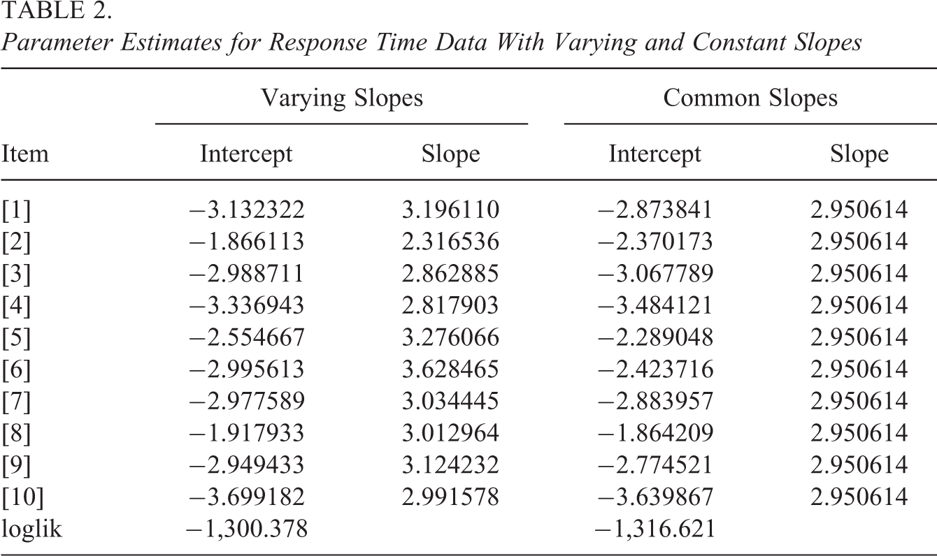
The fit of the model could additionally be improved by allowing for varying discrimination parameter. The corresponding log-likelihood was −1,296.027; however, it does not significantly improve the fit (log-likelihood test is 8.702 on 9 df). Note that picking (solely) on significance is in general not advised, as for large sample size, even smallest improvements become significant. 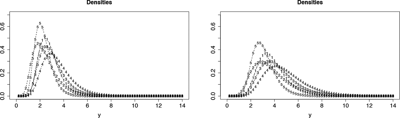Figure 6 shows the estimated response distributions for the first five items for $θ_{p} = 0.0$ (left) and $θ_{p} = 1.0$ (right) for the normal response function and varying slopes.

Figure 6.

Response distributions for the first five items of the mental rotation data set for $θ_{p} = 0.0$ (left) and $θ_{p} = 1.0$ (right).

6.3. Political Fears

In this application, Likert-type scales are considered. We use data from the German Longitudinal Election Study, which is a long-term study of the German electoral process (Rattinger et al., 2014). The data we are using originate from the pre-election survey for the German federal election in 2017 and consist of responses to various items addressing political fears. The participants were asked: “How afraid are you due to the…”—(1) refugee crisis?—(2) global climate change?—(3) international terrorism?—(4) globalization?—(5) use of nuclear energy? The answers were measured on Likert-type scales from 1 (not afraid at all) to 7 (very afraid). The model is fitted under the assumption that fear is the dominating latent trait, which is considered as unidimensional. We use 200 persons sampled randomly from the available set of observations.

Within the thresholds modeling framework, the restriction to a finite interval $(a, b)$ can be obtained by using the logit difficulty function $g (y) = log ((y - a) / (b - y))$ . When approximating a Likert-type scale with values $1, \dots, k$ by continuous distributions, it is not sensible to define the logit function for the interval $(1, k)$ since it excludes the extreme values 1 and k. To include them, the interval has to be enlarged. Therefore, when fitting a continuous response model, we use the interval $(1 - c, k + c)$ , where c is a constant. When fitting a discrete threshold model, the symmetric widening of the interval is not appropriate because the difficulty function should tend to infinity at the upper boundary or at least close to the upper boundary. Therefore, in the discrete case, we use the interval $(1 - 2 c, k + 0.01)$ . In the application, we used $c = 0.5$ , which yields the interval $(0.5, 7.5)$ for continuous modeling and $(0, 7.01)$ for discrete modeling. Smaller values of c yield worse fits in discrete models, but for larger values, the fits are practically the same. For larger values of c, also the approximation of the discrete model by continuous modeling becomes worse.

Figure 7 shows the resulting distributions for alternative assumptions concerning the distribution of responses. The first row shows the fitted densities if one assumes a normal distribution, which is equivalent to a normal distribution CTT model, and the second row shows the densities for the thresholds model with logistic difficulty function. The left side shows the distributions for a low value of the person parameter, and the right side shows the distributions for a high value of the person parameter. 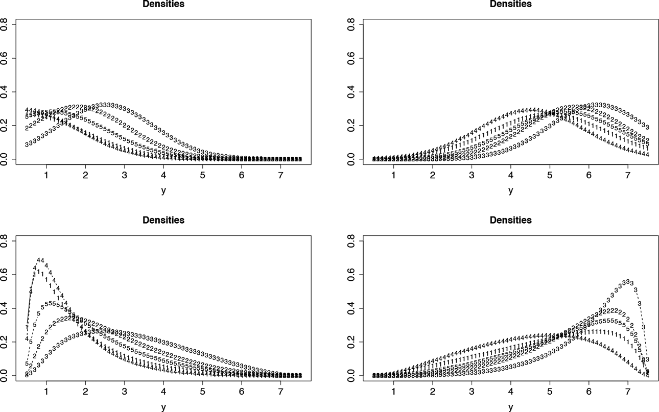Obviously, the normal model does not yield proper distributions since the support of the distributions is much larger than the interval $(1, 7)$ . When using the thresholds model with the logistic difficulty function, the resulting distributions are much more adequate. It illustrates that when using a continuous model for Likert-type data, classical model assumptions as the normal distribution are far off the target.

Figure 7.

Estimated densities for fear data. Left: low person parameter, right: high person parameter, first row: normal distribution model corresponding to linear difficulty functions ( $θ_{low} = - 2.5$ and $θ_{high} = 0.5$ ), and second row: proper restrictions by using logit difficulty functions $θ_{low} = - 1.8$ and $θ_{high} = 0.5$ ). In all cases, the response function is fixed as the normal cdf.

Table 3 shows the log-likelihoods, the AIC values, and estimates of $σ_{θ_{p}}$ for various responses and difficulty functions. The models have varying slopes in the difficulty functions and fixed discrimination parameters since varying discrimination parameters did not improve the fit significantly. We considered two fits, assuming that the responses are continuous or discrete. The latter means that one assumes a multinomial distribution for the responses, which changes the likelihood. It is seen that in both cases, the logit difficulty function always fits better than linear or logarithmic functions. The problems with the latter two have already been illustrated in Figure 7. The best fit is obtained when combining logit difficulty functions with a logistic response function, although normal and Gumbel response functions yield rather similar results.

Table 3.

Thresholds Models for Fears Data

		Continuous			Discrete
Response fct	Diff fct	Log-Lik	AIC	${\hat{σ}}_{θ_{p}}$	Log-Lik	AIC	${\hat{σ}}_{θ_{p}}$
Normal	Linear	−1,847.53	3,717.061	0.707	−1,847.698	3,717.396	0.722
	Log	−2,046.301	4,114.602	0.719	−2,064.723	4,151.440	0.758
	Logit	−1,703.461	3,428.921	0.705	−1,735.862	3,493.724	0.752
Logistic	Linear	−1,849.513	3,721.026	1.343	−1,822.079	3,666.158	1.390
	Log	−2,000.54	4,023.08	1.331	−2,024.321	4,070.643	1.384
	logit	−1,700.976*	3,423.952*	1.327	−1,728.913*	3,479.826*	1.339
Gumbel	Linear	−1,817.634	3,657.269	0.799	−1,819.489	3,660.978	0.830
	Log	−1,891.852	3,805.704	0.629	−1,915.859	3,853.718	0.619
	Logit	−1,704.79	3,431.579	0.856	−1,734.455	3,490.910	0.915
Gompertz	Linear	−1,923.348	3,868.695	0.885	−1,917.457	3,856.913	0.913
	Log	−2,178.687	4,379.374	1.083	−2,179.356	4,380.712	1.174
	Logit	−1,759.693	3,541.386	0.918	−1,759.058	3,540.115	0.883
Graded resp					−1,707.573	3,477.146

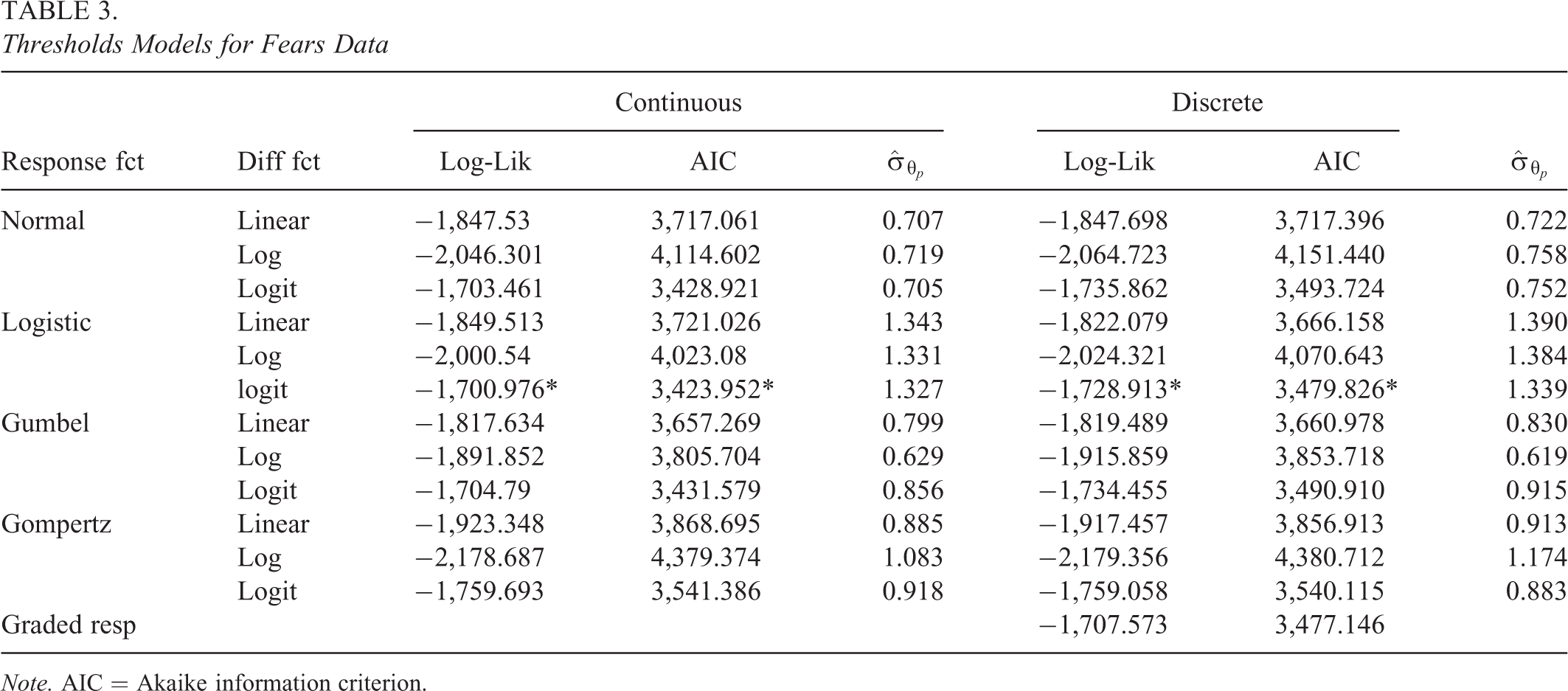
Note. AIC = Akaike information criterion.

We considered continuous and discrete fits since for Likert-type scales with at least five categories continuous models are often used (see, e.g., Harpe, 2015). Therefore, it seems sensible to investigate whether the approximation is warranted. In this application, although the fits for discrete and continuous models differ, in both cases, the same models turn out to be the best models when using the log-likelihood or AIC as criterion. For a further evaluation of the difference between continuous and discrete modeling, we computed the posterior estimates of person parameters. Figure 8 shows the estimates plotted against the transformed sum scores $Y_{p +}^{(δ)}$ using logit transformed data (difficulty function) and Gumbel response function. It is seen that the pictures for continuous and discrete responses are virtually the same. Correspondingly, the correlation between estimated person parameters for discrete and continuous data was 0.996. The correlation between transformed sum scores and estimated parameters was 0.991 for the continuous model and 0.988 for the discrete model. Thus, in this example, in terms of model selection as well as prediction of person parameters, there seems to be no relevant difference between assuming a continuous distribution or a discrete distribution, although the concrete log-likelihoods differ for discrete and continuous distributions.

Figure 8.

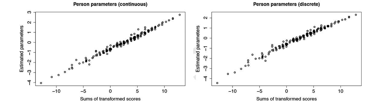
Estimated person parameters for fears data.

Nevertheless, Likert-type scales are by definition discrete, and the approximation by continuous distributions cannot in general be assumed to be sufficiently accurate. General recommendations like the one that “numerical response formats with at least five categories may generally treated as continuous data” (Harpe, 2015) should be viewed with skepticism since the accuracy of the approximation may depend on the distribution of individuals, in the case of thresholds models on the distribution of person parameters. Within the thresholds model framework, one can fit continuous as well as discrete responses and compare the resulting fits and predictions. Alternatives that explicitly account for the discreteness of the response are ordinal IRT models as the graded response model (Samejima, 2016), which can be given by $P (Y_{p i} > r | θ_{p}, α_{i}, δ_{i r}) = F (α_{i} (θ_{p} - δ_{i r}))$ , $r = 1, \dots, k - 1$ if $Y_{p i} \in {1, \dots, k}$ . Note that this model can also be derived via a latent continuous FA model with thresholds on the continuum (Lee, 2007). The general thresholds model with the assumption of discrete responses is equivalent to the graded response model with the threshold parameter of the graded response model given by $δ_{i r} = δ_{i} (r)$ . The (discrete) threshold models with fixed difficulty functions as the linear or logit function are the submodels of the graded response model, and they just restrict the thresholds by assuming that they are determined by a fixed function. Thus, the models have fewer parameters than the graded response model. Table 3 also shows the results if a graded response model with a logistic response function is fitted. The resulting log-likelihood is smaller than for the thresholds model with logistic response function and logit difficulty function, but the difference in AIC values, which takes the number of parameters into account, is minor (3,479.826 compared to 3,477.146).

For the distribution of person parameters and for further comparisons of discrete and continuous modeling strategies, we refer the reader to the Online Appendix.

7. Extensions and Alternative Models

7.1. Including Covariates

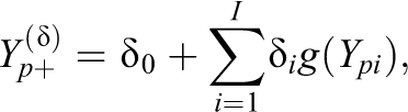
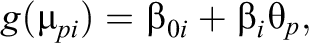
The basic threshold model assumes that latent traits are unidimensional and not affected by covariates. If one suspects that covariates may modify the response behavior, it can be tested by including them explicitly in the explanatory term. Let $x_{p}$ be a person-specific vector of covariates. In a threshold model with covariates, the person parameter $θ_{p}$ is replaced by $θ_{p} - x_{p}^{T} γ_{i}$ yielding

P (Y_{p i} > y | θ_{p}, α_{i}, δ_{i} (.)) = F (α_{i} (θ_{p} - x_{p}^{T} γ_{i} - δ_{i} (y))),

where the parameter $γ_{i}$ is item-specific and represents the effect on the response in item i.

Within IRT, the inclusion of covariates can be seen as investigating differential item functioning (DIF), which is the well-known phenomenon that the probability of a correct response among equally able persons may differ in subgroups (see, e.g., Magis et al., 2010; Millsap & Everson, 1993; Osterlind & Everson, 2009; Rogers, 2005; Zumbo, 1999). If $γ_{i}$ is nonzero, the item functions differently in subgroups represented by covariates.

Model (13) can also be seen as a rather general multivariate regression model with heterogeneity. Models of this type have been considered within the framework of explanatory item response modeling (De Boeck & Wilson, 2004, 2016). If one is primarily interested in the effects of covariates, one considers $θ_{p}$ as representing the heterogeneity needed to model the effects adequately. It can be seen as a generalized random effects model, but with much weaker assumptions on the distribution of the response variables than in the classical linear mixed model (Goldstein, 1987; Searle et al., 1992).

Let us consider the fear data with covariates gender (1: female; 0: male) and age in years. Table 4 shows the estimates for the basic model without covariates and the model with covariates age and gender (discrete response, $α_{i} = 1$ , logistic response function, and logit difficulty function). It is seen that all items show significant covariate effects for at least one of the covariates (z values given in the last two columns). Older respondents tend to be more afraid than younger respondents, females have for all items higher fear levels than males. The necessity of covariates is also supported by testing. The log-likelihood test that compares the model without covariates to the model with covariates is 373.980 on 10 df. Thus, if one considers it as a DIF problem, all items show DIF. From a regression perspective, gender and age are seen to be influential if one accounts for the heterogeneity in the population.

Table 4.

Parameter Estimates for the Fears Data With Logit Difficulty Function, Logistic Response Function Without Covariates and With Covariates

		Parameters				z Values
	Item	Intercepts	Slopes	Age	Gender	z-Age	z-Gender
1		−0.255	1.575
2		−1.391	1.834
3		−2.153	1.644
4		0.225	1.789
5		−0.837	1.655
	Log-lik	−1,728.913
1	Refugee	0.204	0.976	−0.012	−0.612	−1.691	−2.134
2	Climate change	−0.691	0.888	−0.005	−0.934	−0.724	−3.236
3	Terrorism	−0.175	0.753	−0.026	−1.268	−3.415	−4.198
4	Globalization	0.705	1.509	−0.014	−0.816	1.871	−2.858
5	Nuclear energy	−0.158	0.881	−0.015	−0.285	−2.052	−0.998
	Log-lik	−1,541.923

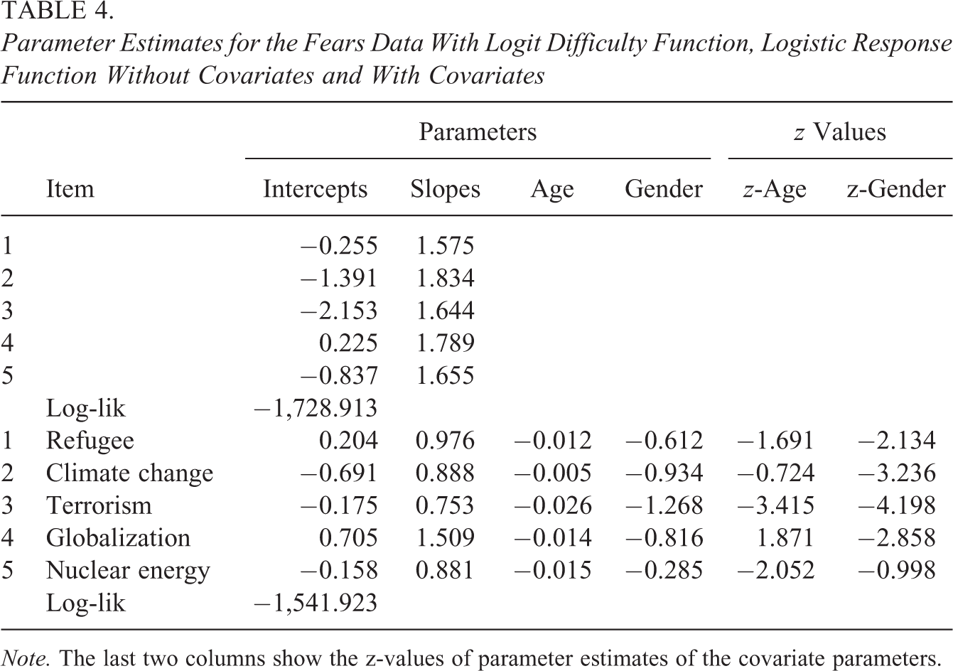
Note. The last two columns show the z-values of parameter estimates of the covariate parameters.

It is seen from Table 3 that difficulty functions that account for the restriction to an interval yield better fits when no covariates are included. If covariates are included, one is typically also interested in the significance of covariates. Then, models that ignore the restriction and therefore work with improper distributions can hardly be trusted to yield reliable results in significance tests. For example, fitting of a normal distribution model with covariates yields for covariate age the z values −2.16, 0.26, −2.94, −2.12, and −1.50 (for Items 1–5), which differ from the values given in Table 4, −1.69, −0.72, −3.41, 1.87, and −2.05. Thus, fitting of models with improper distributions might yield misleading results in significance tests.

7.2. Alternative Models

7.2.1. Generalized linear IRT (GLIRT)

Mellenbergh (1994) proposed a GLIRT and a corresponding comprehensive class of models. In essence, the model assumes that a monotone differentiable transformation g of the expected value $μ_{p i}$ is linked to a linear predictor of latent (and manifest variables) via

g (μ_{p i}) = β_{0 i} + β_{i} θ_{p},

where for the sake of simplicity, we have confined the model description to a unidimensional latent variable model without covariates. In addition to this link function, a response function from an exponential family is assumed for the conditional distribution of $Y_{p i}$ , thereby essentially arriving at a modeling approach akin to generalized linear models (McCullagh & Nelder, 1989).

If responses are multinomially distributed, some modifications toward vectorized expectations are necessary to adopt the model to fit traditional polytomous IRT models. Polytomous responses are not one-dimensional; therefore, the transformation of expected responses is less simple since one has a vector of response and therefore a vector of expectations referring to the probabilities of specific categories. By appropriate modification, classical response models as the graded response model and the partial credit model can be shown to be special cases. Threshold model also contains generalized graded response models as special cases but not the partial credit model. For discrete responses with infinite support, GLIRT type models have been considered by Wang (2010), also assuming a fixed distribution, Poisson with zero inflation. Also, in this case, threshold type models are not restricted to fixed distributions (see Tutz, 2022a).

While in thresholds models, the distribution is a result of the response function and the difficulty function in GLRIT models a distribution is assumed and the link refers to the expected value. Although many models in current use can be represented as GLRIT models for continuous responses, they are less flexible. In particular, the restriction to an interval is hard to obtain. When considering Likert-type scales as approximations to continuous responses, Mellenbergh (1994) refers to the normal distribution. The strength of thresholds models is that they can adapt very flexibly to the demands of item formats without having to assume a fixed distribution for responses.

7.2.2. Factor analysis

Another approach to the modeling of continuous responses, though not commonly subsumed under the IRT framework, is given by the class of FA (or more generally: structural equation models) models. Within this approach, the evaluation metric and oftentimes also the model fitting differs from the IRT framework. More specifically, FA is mostly focused on the reproduction of the covariance matrix of the manifest variables (Mardia et al., 1979). This in turn is reflected in model fitting approaches, which may rely on minimizing a weighted least squares distance between the model implied and the observed covariance matrices (Du & Bentler, 2021). Despite these differences, there is, however, a connection between the commonly employed FA models and our TM IRT model. To highlight this connection, we assume a unidimensional FA model of the form

Y_{p i} = μ_{i} + α_{i} θ_{p} - ε_{p i},

with the assumption that conditionally on the factor $θ$ , the residual terms $ε_{p i}$ (the uniqueness terms) are independent of each other. If G_i denotes the absolutely continuous cumulative distribution function of $ε_{i}$ , then $P (Y_{p i} > y | θ_{p})$ can be computed as follows:

P (Y_{p i} > y | θ_{p}) = P (- ε_{p i} > y - μ_{i} - α_{i} θ_{p} | θ_{p}),

= P (ε_{p i} \leq α_{i} θ_{p} + μ_{i} - y | θ_{p}) = G_{i} (α_{i} θ_{p} + μ_{i} - y) .

If the G_i originates from a common location scale family, that is, if $G_{i} (v) : = G (\frac{v - a}{b})$ holds, then we arrive at a TM model with a linear difficulty function and G as the response function of the ith item. It is just given in a slightly different parameterization, which is seen from the thresholds model representation $P (Y_{p i} > y) = F (α_{i} (θ_{p} - δ_{0 i} - δ_{i} g (y))) = F (α_{i} θ_{p} - {\tilde{δ}}_{0 i} - {\tilde{δ}}_{i} g (y))$ , where ${\tilde{δ}}_{0 i} = α_{i} δ_{0 i}$ and ${\tilde{δ}}_{i} = α_{i} δ_{i}$ .

Therefore, the FA model (with a flexible choice for the distribution of the residual term) can be subsumed under the TM family. This holds also for multifactor models, in which $α_{i} θ_{p}$ is replaced by $α_{i}^{T} θ_{p}$ , where $α_{i}^{T} = (α_{i 1}, \dots, α_{i m})$ is a m-dimensional factor with loadings $θ_{p}^{T} = (θ_{p 1}, \dots, θ_{p m})$ .

Note, however, that fitting a model with the standard factor analytical framework presupposes normality of the residuals. There are methods for the corrections of standard errors in the presence of nonnormality. Nevertheless, the fitting of a TM will result in more efficient estimates due to the fact that the TM estimates are derived via maximum likelihood, whereas the FA based estimates are only maximum likelihood estimates in the presence of normality.

8. Concluding Remarks

The topic of latent trait modeling for continuous responses has been addressed within the framework of threshold models. With respect to continuous responses, the lognormal and the normal-linear model (the basic building block in the FA model) have been shown to be the members of the thresholds modeling class. Furthermore, a better approximation to the handling of Likert-type data has been suggested via the usage of appropriately chosen nonlinear difficulty functions. It has also been demonstrated that response functions other than the normal distribution can be more appropriate.

Future research could focus on multidimensional extensions of the TM class, which would ultimately provide a latent trait model for multidimensional abilities and continuous responses. Alongside these multidimensional extensions, the modeling of data for mixed measurement levels also becomes important. For instance, response times are usually recorded in conjunction with the accuracy of the response (correct/incorrect). A proper approach would need to model the joint distribution of $(x_{i}, t_{i})$ (with x_i denoting the binary indicator of a correct response) in terms of a multidimensional trait encompassing a speed and an accuracy component. Finally, it should be emphasized that for continuous responses, the sensitivity of parameter estimates with respect to extreme responses becomes of extra importance. That is, when using these models for the classification of persons, it has to be ruled out that extreme responses on single items show large effects on the estimate of the ability parameter. The answer to this question might depend on the choice of the difficulty function and the choice of the response function in the TM model and is an additional topic of future research.

Supplemental Material

Supplemental Material, sj-pdf-1-jeb-10.3102_10769986231184147 - Latent Trait Item Response Models for Continuous Responses

Supplemental Material, sj-pdf-1-jeb-10.3102_10769986231184147 for Latent Trait Item Response Models for Continuous Responses by Gerhard Tutz and Pascal Jordan in Journal of Educational and Behavioral Statistics

Footnotes

Appendix

Declaration of Conflicting Interests

The author(s) declared no potential conflicts of interest with respect to the research, authorship, and/or publication of this article.

Funding

The author(s) received no financial support for the research, authorship, and/or publication of this article.

ORCID iD

Gerhard Tutz

References

Barndorff-Nielsen

O. E.

Shiryaev

A. N.

(2015). Change of time and change of measure, Volume 21. World Scientific Publishing Company.

De Boeck

Wilson

(2004). A framework for item response models. In P. De Broeck & M. Wilson (Eds.), Explanatory item response models. A generalized linear and nonlinear approach (pp. 3–41). New York, NY: Springer. https://doi.org/10.1007/978-1-4757-3990-9_1

De Boeck

Wilson

M. R.

(2016). Explanatory response models. In Van der Linden

(ed.), Handbook of item response theory, Volume 1 (pp. 593–608). Chapman and Hall/CRC.

Bentler

P. M.

(2021). Distributionally weighted least squares in structural equation modeling. Psychological Methods, 27(4), 519–540.

Ferrando

P. J.

Lorenzo-Seva

(2007). An item response theory model for incorporating response time data in binary personality items. Applied Psychological Measurement, 31(6), 525–543.

Goldstein

(1987). Multilevel Models in Educational and Social Research. London and Oxford University Press.

Harpe

S. E.

(2015). How to analyze Likert and other rating scale data. Currents in pharmacy teaching and learning 7(6), 836–850.

Hemker

B. T.

Sijtsma

Molenaar

I. W.

Junker

B. W.

(1997). Stochastic ordering using the latent trait and the sum score in polytomous IRT models. Psychometrika, 62(3), 331–347.

Hemker

B. T.

van der Ark

L. A.

Sijtsma

(2001). On measurement properties of continuation ratio models. Psychometrika, 66(4), 487–506.

10.

Holland

P. W.

Hoskens

(2003). Classical test theory as a first-order item response theory: Application to true-score prediction from a possibly nonparallel test. Psychometrika, 68(1), 123–149.

11.

Holland

P. W.

Rosenbaum

P. R.

(1986). Conditional association and unidimensionality in monotone latent variable models. The Annals of Statistics, 1523–1543.

12.

Jackson

P. H.

Agunwamba

C. C.

(1977). Lower bounds for the reliability of the total score on a test composed of non-homogeneous items: I: Algebraic lower bounds. Psychometrika, 42(4), 567–578.

13.

Lakes

K. D.

Hoyt

W. T.

(2009). Applications of generalizability theory to clinical child and adolescent psychology research? Journal of Clinical Child & Adolescent Psychology, 38(1), 144–165.

14.

Lee

S.-Y.

(2007). Structural equation modeling: A Bayesian approach. John Wiley & Sons.

15.

Lord

F. M.

Novick

M. R.

(2008). Statistical theories of mental test scores. IAP.

16.

Magis

B’eland

Tuerlinckx

Boeck

(2010). A general framework and an r package for the detection of dichotomous differential item functioning. Behavior Research Methods, 42(3), 847–862.

17.

Mair

(2018). Modern psychometrics with R. Springer.

18.

Mardia

Kent

Bibby

(1979). Multivariate analysis, 1979. In Probability and mathematical statistics. Academic Press Inc.

19.

Masters

G. N.

(1982). A Rasch model for partial credit scoring. Psychometrika, 47, 149–174.

20.

McCullagh

Nelder

J. A.

(1989). Generalized linear models (2nd ed.). Chapman & Hall.

21.

Mellenbergh

G. J.

(1994). Generalized linear item response theory. Psychological Bulletin, 115(2), 300.

22.

Millsap

Everson

(1993). Methodology review: Statistical approaches for assessing measurement bias. Applied Psychological Measurement, 17(4), 297–334.

23.

Novick

M. R.

(1966). The axioms and principal results of classical test theory. Journal of Mathematical Psychology, 3(1), 1–18.

24.

Osterlind

Everson

(2009). Differential item functioning (Vol. 161). Sage Publications, Inc.

25.

Rasch

(1960). Probabilistic models for some intelligence and attainment tests. Danish Institute for Educational Research.

26.

Rattinger

Roßteutscher

Schmitt-Beck

Weßels

Wolf

(2014). Pre-election cross section (GLES 2013). GESIS Data Archive, Cologne ZA5700 Data file Version 2.0.0.

27.

Raykov

(1997). Estimation of composite reliability for congeneric measures. Applied Psychological Measurement, 21(2), 173–184.

28.

Rhemtulla

Brosseau-Liard

P. É.

Savalei

(2012). When can categorical variables be treated as continuous? A comparison of robust continuous and categorical Sem estimation methods under suboptimal conditions. Psychological Methods, 17(3), 354.

29.

Rogers

HJ.

Differential item functioning. In B. S. Everitt & D. C. Howell (Eds.), Encyclopedia of statistics in behavioral science (pp. 485–490). John Wiley & Sons, Ltd.

30.

Roskam

E. E.

(1997). Models for speed and time-limit tests. In Handbook of modern item response theory (pp. 187–208). Springer.

31.

Samejima

(2016). Graded response model. In Van der Linden

(Ed.), Handbook of item response theory (pp. 95–108). CRC Press.

32.

Searle

Casella

McCulloch

(1992). Variance components. Wiley.

33.

Sijtsma

Hemker

B. T.

(2000). A taxonomy of IRT models for ordering persons and items using simple sum scores. Journal of Educational and Behavioral Statistics 25(4), 391–415.

34.

Sijtsma

Molenaar

I. W.

(2002). Introduction to nonparametric item response theory (Vol. 5). Sage.

35.

Tutz

(2022a). A flexible item response models for count data: The count thresholds model. Applied Psychological Measurement, 46, 643–661.

36.

Tutz

(2022b). Item response thresholds models: A general class of models for varying types of items. Psychometrika, 87, 1238–1269.

37.

van der Linden

W. J.

(2006). A lognormal model for response times on test items. Journal of Educational and Behavioral Statistics, 31(2), 181–204.

38.

van der Linden

W. J.

(2016). Lognormal response-time model. In Handbook of Item Response Theory (Vol. 1; pp. 289–310). Chapman and Hall/CRC. doi:10.1007/978-1-4757-2691-6

39.

Wang

(2010). Irt–zip modeling for multivariate zero-inflated count data. Journal of Educational and Behavioral Statistics, 35(6), 671–692.

40.

Widder

D. V.

(2015). Laplace transform (PMS-6). Princeton University Press.

41.

Zumbo

(1999). A handbook on the theory and methods of differential item functioning (DIF) (pp.1–57). National Defense Headquarters.

Supplementary Material

Please find the following supplemental material available below.

For Open Access articles published under a Creative Commons License, all supplemental material carries the same license as the article it is associated with.

For non-Open Access articles published, all supplemental material carries a non-exclusive license, and permission requests for re-use of supplemental material or any part of supplemental material shall be sent directly to the copyright owner as specified in the copyright notice associated with the article.

0.00 MB

0.26 MB