Sage Journals: Discover world-class research

Abstract

Bayesian methods to infer model dimensionality in factor analysis generally assume a lower triangular structure for the factor loadings matrix. Consequently, the ordering of the outcomes influences the results. Therefore, we propose a method to infer model dimensionality without imposing any prior restriction on the loadings matrix. Our approach considers a relatively large number of factors and includes auxiliary multiplicative parameters, which may render null the unnecessary columns in the loadings matrix. The underlying dimensionality is then inferred based on the number of nonnull columns in the factor loadings matrix, and the model parameters are estimated with a postprocessing scheme. The advantages of the method in selecting the correct dimensionality are illustrated via simulations and using real data sets.

Keywords

Gibbs sampling model dimensionality ordering dependence sparsity spike-slab prior

Introduction

Factor analytic models are widely used in fields such as behavioral science, medical research, and financial studies. The main purpose of factor analysis is to describe the dependence among a set of outcomes in terms of a lower number of latent factors. Compared with the frequentist setting, Bayesian factor analysis provides more flexibility to fit models across different scenarios (Lee & Song, 2002). In the frequentist setting, exploratory factor analysis is carried out as a multistep approach when the number of factors is unclear. First, model dimensionality is selected, and then, factor rotation is conducted to obtain model simplicity and interpretability. This multistep approach is theoretically suboptimal due to the possible loss of information between steps, especially taking into account the variety of methods for factor extraction and factor rotation, each with its own pros and cons (Chen, 2021).

In contrast, Bayesian methods can simultaneously conduct model selection and parameter estimation in factor analysis (e.g., Carvalho et al., 2008; Conti et al., 2014; Mavridis & Ntzoufras, 2014). However, these Bayesian approaches generally assume a lower triangular structure for the factor loadings matrix in order to ensure identifiability of the models. As discussed in Carvalho et al. (2008), when using this restriction for model identification, the order of the variables introduces unintended prior information, which may influence the results when inferring model dimensionality. Chen (2021) proposed a Bayesian regularized approach to exploratory factor analysis (BREFA) without assuming a lower triangular structure for the factor loadings matrix. In this method, the constraints for model identifiability are imposed on the factor covariance matrix. Alternatively, to overcome the dependence on the order of the outcomes, Man and Culpepper (2022) introduced a permuted positive lower triangular restriction to address rotational invariance. The authors introduced a Bayesian sampling algorithm that explores the multimodal posterior surface of the factor loadings matrix. Nonetheless, this approach does not perform automatic selection of the number of factors.

We propose a method to select model dimensionality in factor analysis without imposing the lower triangular condition for model identifiability. Our approach considers a model with a relatively large number of factors and includes auxiliary multiplicative parameters, which may render null the unnecessary columns in the factor loadings matrix. We introduce a peaked and heavy-tailed prior that induces sparsity on the auxiliary parameters. Hence, the underlying dimensionality is inferred based on the number of nonnull columns in the factor loadings matrix. The specification of this proposal permits its easy implementation in Bayesian packages. We solve rotational indeterminacy to estimate the model parameters using the postprocessing scheme in Papastamoulis and Ntzoufras (2022).

To decide which columns are nonnull in the factor loadings matrix, we make use of the spike-slab prior, which is a popular tool in Bayesian model selection. Mitchell and Beauchamp (1988) introduced the spike-slab distribution in Bayesian variable selection as the mixture of a point mass at zero and a uniform distribution, in order to determine which regression coefficients are null in linear regression models. George and McCulloch (1993) proposed a modification, which simplifies Gibbs sampling by taking as prior a mixture of two normal distributions with different variances. Alternatively, Kuo and Mallick (1998) suggested a mixture of a point mass at zero and a normal distribution to avoid the need of choosing the variance of the normal component corresponding to the spike in George and McCulloch (1993).

Mavridis and Ntzoufras (2014) developed a Markov chain Monte Carlo (MCMC) algorithm based on the prior of George and McCulloch (1993) for estimating the factor model and identifying promising subsets of manifest variables. Pan et al. (2021) extended this methodology to investigate latent risk factors of mixed type of outcomes. On the other hand, proposals such as Lucas et al. (2006), Carvalho et al. (2008), Conti et al. (2014), Ročková and George (2016), Frühwirth-Schnatter and Lopes (2018), and the Indian buffet process in Ghahramani and Griffiths (2005) carry out Bayesian factor analysis using sparsity mixture priors based on Kuo and Mallick (1998). This avoids choosing the variance of the normal component for the spike in George and McCulloch (1993), but sampling from the posteriors is more involved due to the point mass at zero component.

We use the spike-slab prior of George and McCulloch (1993) to decide which elements are nonnull in the factor loadings matrix, similarly as in Mavridis and Ntzoufras (2014) and Pan et al. (2021). This leads to a simple MCMC estimation procedure because the conditional posteriors for Gibbs sampling correspond to closed-form distributions. In addition, Bayesian methods for exploratory factor analysis in the literature assign a spike-slab prior to each factor loading in order to determine which elements are null in the factor loadings matrix (see, e.g., Lucas et al., 2006; Carvalho et al., 2008; Conti et al., 2014; Ročková & George, 2016; Chen, 2021). In contrast, our approach assigns a spike-slab prior to a parameter that multiplies each column in the factor loadings matrix. As we illustrate, this may lead to more power for inferring the number of factors since it is not necessary to determine whether each single factor loading is non-null. Instead, our approach uses the information of the full column of factor loadings to determine whether the full column is null or not.

The outline of this article is as follows. First, we discuss the general factor analytic model and a sparse representation for overfitted models. Then, the proposed prior is introduced and the Gibbs procedure to infer the number of factors is discussed together with the identifiability of the model. Finally, we demonstrate the advantages of our proposal via simulations and illustrate the method using real data sets.

Factor Model Specification

The factor analytic model assumes that each p-dimensional observation $y_{i}$ can be explained by a m-dimensional vector $η_{i} \sim N_{m} (0, I_{m})$ of standard normal latent factors as follows:

y_{i} = Δ η_{i} + ∊_{i},

where $Δ$ is a $p \times m$ matrix of factor loadings, $∊_{i} \sim N_{p} (0, Σ)$ is a residual vector with diagonal covariance matrix $Σ = diag (σ_{1}^{2}, \dots, σ_{p}^{2})$ , and $η_{i}$ is independent from $∊_{i}$ for $i = 1, \dots, n$ . For simplicity in exposition, we leave the intercept out of Equation 1.

The marginal distribution of $y_{i}$ integrating out the latent factors is $N_{p} (0, Ω)$ with $Ω = Δ Δ^{'} + Σ$ . Hence, given the diagonal structure of $Σ$ , the dependence in the outcomes is exclusively explained by the common latent factors. In practice, the number of factors is smaller than the number of outcomes ( $m < p$ ), since factor analysis is generally a dimension reduction technique.

Geweke and Singleton (1980) proved that when the factor loadings matrix is not of full rank, that is, the true number of factors is $r = rank (Δ) < m$ , the parameters in $Σ$ are underidentified. Indeed, let $R$ be a $m \times (m - r)$ matrix, such that $Δ R = 0_{p \times (m - r)}$ and $R' R = I_{m - r}$ . Then

Ω = Δ Δ^{'} + Σ = (Δ + M R^{'}) (Δ + M R^{'})^{'} + (Σ - M M^{'}),

for any $p \times (m - r)$ matrix $M$ with mutually orthogonal rows. Hence, identification problems arise when fitting factor models with a number of factors m larger than the true number of underlying factors r. This represents a serious problem because it is not possible to determine a priori the maximum value of m that should be considered in practice. Therefore, when comparing the models of dimensionality 1, 2, $\dots$ , m using standard Bayesian approaches, the inference will generally be based on MCMC samples from identifiable models with 1, $\dots$ , r factors and from nonidentified models with $r + 1$ , $\dots$ , m factors. This may affect the validity of the results (Lopes & West, 2004) in a similar way as for the likelihood ratio test (LRT) in the frequentist setting (Hayashi et al., 2007).

Sparse Model Representation

Instead of considering the lack of identifiability in Equation 2 as a difficulty in factor analysis, we use it as a tool in our approach to determine model dimensionality. For this, we show that if the true number of factors is $r < m$ , there exists a rotated solution of the factor model, where the factor loadings matrix has $m - r$ null columns.

It is well known that for any $m \times m$ orthogonal matrix $P$ , the model in Equation 1 can be re-expressed by its rotated solution $y_{i} = Δ P η_{i}^{*} + ∊_{i}$ with $η_{i}^{*} = P' η_{i}$ . Let us assume that the model is overfitted and the true number of underlying factors is $r < m$ . As before, let $R$ be a $m \times (m - r)$ matrix, such that $Δ R = 0_{p \times (m - r)}$ and $R' R = I_{m - r}$ , and let $Q$ be any $m \times r$ matrix for which $Q' Q = I_{r}$ and $Q' R = 0_{r \times (m - r)}$ . Then, the block matrix $P = [Q_{m \times r} R_{m \times (m - r)}]$ is orthogonal and Equation 1 can be re-expressed as

y_{i} = Δ [Q_{m \times r} R_{m \times (m - r)}] η_{i}^{*} + ∊_{i} = [Δ Q_{m \times r} 0_{p \times (m - r)}] η_{i}^{*} + ∊_{i} .

This result is intuitive. For overfitted models, there must exist a rotated solution in which, for the unnecessary factors, the columns of the factor loadings matrix are null. We introduce auxiliary parameters $ν_{1}, \dots, ν_{m}$ that control which of the m columns are null in the factor loadings matrix. More specifically, we fit the factor model

y_{i} = (\begin{matrix} ν_{1} δ_{1} & \dots & ν_{m} δ_{m} \end{matrix}) η_{i} + ∊_{i} = Δ N η_{i} + ∊_{i},

with factor loadings matrix $Δ N$ , where $δ_{k} = (δ_{1 k}, \dots, δ_{p k})^{'}$ corresponds to the $k th$ column of $Δ$ ( $k = 1, \dots, m$ ) and $N = diag (ν_{1}, \dots, ν_{m})$ . Notice that when $ν_{k} = 0$ , the $k th$ column $ν_{k} δ_{k}$ of the factor loadings matrix is rendered null in Equation 4.

From Equation 3, we know that if the number of factors is $r \leq m$ , there exists a solution of the model in Equation 4 with r nonnull columns in the factor loadings matrix, that is, $\sum_{k} I {ν_{k} \neq 0} = r$ . For all other rotated solutions, we will have $\sum_{k} I {ν_{k} \neq 0} \geq r$ . Our approach for inferring dimensionality in factor analysis (IDIFA) employs the inferential model in Equation 4, inducing prior sparsity for the $ν_{k}$ components to obtain the representation in Equation 3 of the model.

The value of m can be selected based on the previous analyses or expert knowledge. In the absence of prior information, m can be chosen as the maximum number of factors leading to an identified model. As explained later, it corresponds to the maximum value of m, such that $p (p + 1) / 2 - p (m + 1) + m (m - 1) / 2 \geq 0$ . This is a necessary, but not sufficient condition for identifiability. The row deletion theorem provides a sufficient condition for identifiability in factor models, see Theorem 5.1 in Anderson and Rubin (1956) for details.

Prior Specification

In the IDIFA approach, we consider the “effective rank” of the factor loadings matrix, that is, the minimum number of columns that are importantly different from null. To approximate the solution in Equation 3 via MCMC methods, we use a similar strategy as in George and McCulloch (1993). Namely, each component of $N$ in Equation 4 is assigned a normal mixture prior based on a binary latent variable $γ_{k}$ as follows:

ν_{k} | γ_{k} : (1 - γ_{k}) N (0, τ_{k}^{2}) + γ_{k} N (0, c_{k}^{2} τ_{k}^{2}) for k = 1, \dots, m,

with $p (γ_{k} = 1) = 1 - p (γ_{k} = 0) = π_{k}$ . The parameters c_k and $τ_{k}$ are fixed. Setting $τ_{k}^{2}$ small and $c_{k}^{2}$ to be large in Equation 5 implies that if $γ_{k} = 0$ , then $ν_{k}$ is very close to zero and when $γ_{k} = 1$ probably $ν_{k} \neq 0$ . It is not straightforward to define in practice what is small and large for c_k and $τ_{k}$ , respectively. An alternative could be to take the prior in Kuo and Mallick (1998) with a point mass at zero, but this leads to serious convergence issues in our approach as discussed in the following. To facilitate the choice of c_k and $τ_{k}$ , we standardize the outcomes in $y_{i}$ to make the procedure unit-independent. See the following section for further details.

The elements $δ_{j k}$ in $Δ$ ( $j = 1, \dots, p$ ; $k = 1, \dots, m$ ) are mutually independent a priori and follow a standard normal prior distribution. We also assume that $δ_{j k}$ is independent from $ν_{k}$ a priori. Thus, from the properties of products of independent normal random variables, we have that the mean for each column of the factor loadings matrix $Δ N$ in Equation 4 is $E (ν_{k} δ_{k} | γ_{k}) = 0_{p}$ and the covariance matrix is

Var (ν_{k} δ_{k} | γ_{k}) = (1 - γ_{k}) {diag(τ}_{k}^{2}, \dots, τ_{k}^{2}) + γ_{k} diag (c_{k}^{2} τ_{k}^{2}, \dots, c_{k}^{2} τ_{k}^{2}) .

Hence, if $γ_{k} = 0$ , all components of $ν_{k} δ_{k}$ in Equation 4 are very small and the corresponding factor is effectively switched off. On the other hand, if $γ_{k} = 1$ , the $k th$ factor appears as important in the model. Therefore, the dimensionality of the model, which is our main interest, can be determined based on the “effective rank” of $Δ N$ , that is, $r_{γ} = \sum_{k} γ_{k}$ . There is no preference for specific columns of the factor loadings matrix a priori, so we assume a constant inclusion probability for all columns, that is, $π_{1} = \dots = π_{m} = π$ . Therefore, $γ_{1}, \dots, γ_{m}$ have an exchangeable prior.

In the IDIFA approach, the inclusion probability $π$ is estimated given the data. We assign a priori $π \sim Beta (a / m, b)$ , where m is the number of potential factors. The rotational invariance in factor models manifests itself through a multimodal posterior, but this source of indeterminacy is ameliorated by promoting factor orientations with many zero loadings (Ročková & George, 2016). Therefore, we select hyperparameters a and b that lead to small values of the inclusion probability $π$ . This leads in turn to a small number of relevant columns $r_{γ}$ a priori and guides the factor loadings matrix $Δ N$ in Equation 4 toward the sparse rotated solution 3. We consider different values for a and b in the simulation study.

Finally, we choose an inverse gamma prior for the idiosyncratic variances, namely, $σ_{1}^{2}, \dots, σ_{p}^{2} : I G (3 / 2, 1 / 4)$ . This choice results in a diffuse prior that decays to zero sufficiently rapid as $σ_{j}^{2}$ tends to zero (Peeters, 2012) and allocates the prior mean in the middle of the interval $[0, 1]$ .

Selecting the Hyperparameters

The density in the slab component corresponds to the distribution of the product of two normal variables, that is, $ν_{k} | (γ_{k} = 1) : N (0, c_{k}^{2} τ_{k}^{2})$ and $δ_{j k} : N (0, 1)$ . Given that these two variables are independent and zero-mean normally distributed, the mean of their product is zero and the variance equals $c_{k}^{2} τ_{k}^{2}$ . The density of this product according to Simon (2007) is

f_{ν_{k} δ_{j k} | γ_{k} = 1} (z) = \frac{1}{π c_{k} τ_{k}} K_{0} (\frac{| z |}{c_{k} τ_{k}}),

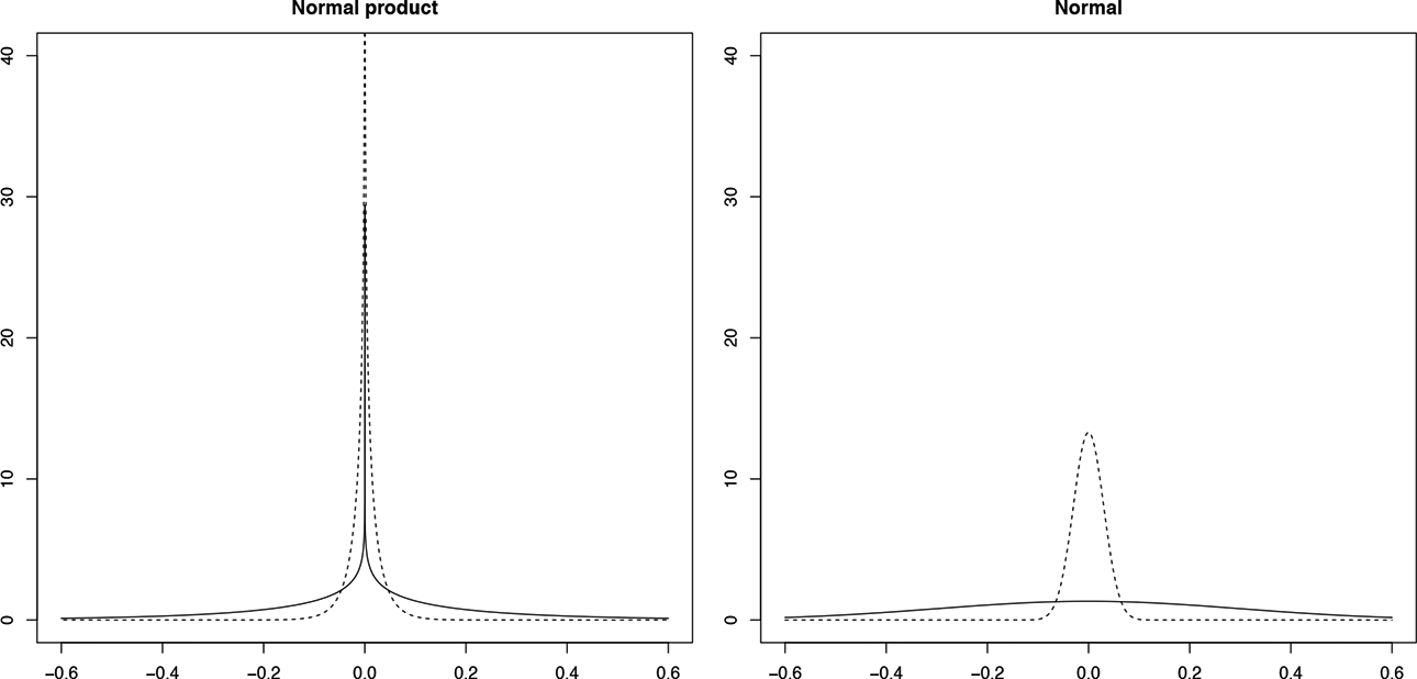
where K ₀ is the modified Bessel function of the second kind and zero order. See Online Appendix A for further details on this modified Bessel function. Similarly, the density for the spike component is $f_{ν_{k} δ_{j k} | γ_{k} = 0} (z) = 1 / ({πτ}_{k}) K_{0} (| z | / τ_{k})$ . The spike and slab densities are presented in Figure 1 (left panel), taking $c_{k} τ_{k} = 0.3$ and $c_{k} = 10$ .

Figure 1.

Marginal prior density for ν _k δ _jk assuming a normal product prior (left) and a normal prior (right). The dotted line corresponds to the spike and the solid line to the slab.

When a factor is not necessary, then $γ_{k} = 0$ and all the corresponding factor loadings are sampled from the spike, which is clustered around zero. Small values of the inclusion probability $π$ maximize the number of nonimportant columns in $Δ N$ and approximate the sparse solution in Equation 3. If a factor is important ( $γ_{k} = 1$ ), the corresponding factor loadings are sampled from the slab component—where it is more likely to have substantial values.

The intersection between the spike and the slab can be regarded as a threshold for declaring practical significance (George & McCulloch, 1993). Using a first-order expansion for the modified Bessel function (Abramowitz & Stegun, 1964), we find that the two densities intersect approximately at $\pm ζ_{k} = c_{k} τ_{k} / (c_{k} - 1) log (\sqrt{c_{k}} (1 - τ_{k}) / (1 - c_{k} τ_{k}))$ , so factor loadings falling into the interval $[- ζ_{k}, ζ_{k}]$ can be regarded as nonrelevant. In the specific case of Figure 1 (left panel), the two densities intersect at $\pm 0.05$ , indicating that the values of the factor loadings $| ν_{k} δ_{j k} | < 0.05$ are considered as nonrelevant under this prior specification. We compare different values for c_k and $τ_{k}$ in the simulation study.

Characteristics of the Prior

The density in Equation 6 goes to infinity as z approaches zero. Therefore, the prior in IDIFA is peaked around zero even for the slab component. This is crucial in our approach because, for important factors with $γ_{k} = 1$ , some of the factor loadings $ν_{k} δ_{j k}$ can still be sampled close to zero. Note that each underlying factor explains some of the outcomes in practice and not all factor loadings need to be considerably large.

For comparison purposes, let us consider for $ν_{k} δ_{j k}$ the spike-slab prior based on a normal mixture as in George and McCulloch (1993). Such a prior can be obtained by assuming that $δ_{j k} : N (0, 1)$ and taking $ν_{k} | γ_{k}$ to be a fixed value, namely, $(1 - γ_{k}) τ_{k} + γ_{k} c_{k} τ_{k}$ for $k = 1, \dots, m$ . In Figure 1 (right panel), we present this prior taking $c_{k} τ_{k} = 0.3$ as the standard deviation of the slab component and $τ_{k} = 0.022$ . The latter value is selected in order to have approximately $\pm 0.05$ as intersection points between the two densities.

The peakedness around zero for the proposed prior in Equation 6 is essential for IDIFA because it reflects that several factor loadings can be null for the underlying factors. In contrast, the prior in Figure 1 (right panel) has lower density around zero for the slab component and $\int_{- x}^{x} f_{ν_{k} δ_{j k} | γ_{k} = 1} (z) d z \approx 0$ for small values of positive x. Therefore, this prior specification would consider factor k as important ( $γ_{k} = 1$ ) only when all factor loadings in the column $ν_{k} δ_{k}$ are substantially different from zero. We found that using such a prior for the factor loadings in IDIFA leads to strong underestimation of the number of factors and mixing problems in Bayesian inference.

Finally, the prior in Equation 6 resulting from the product of two normal variables is a heavy-tailed distribution (Guo, 2017). For instance, when generating a sample of $100,000$ observations for $ν_{k}$ and $δ_{j k}$ , the $99.5 %$ empirical quantile of $ν_{k} δ_{j k}$ taking $c_{k} τ_{k} = 0.3$ is approximately $1.09$ , while the corresponding quantile assuming a normal density equals $0.77$ .

Inferring the Number of Factors

Gibbs Sampling

In the IDIFA approach, it is not necessary to fit all models with $0, 1, \dots, m$ factors in order to select the correct dimensionality. Instead, we fit only the model in Equation 4 and the number of underlying factors is inferred based on the posterior distribution of $r_{γ} = \sum_{k} γ_{k}$ . All prior distributions are conditionally conjugate in IDIFA, so the conditional posteriors for Gibbs sampling correspond to closed-form distributions. These are reported in Online Appendix B.

We take values a and b, such that the prior $π : Beta (a / m, b)$ is concentrated in small values close to zero. This induces sparsity in the factor loadings matrix and guides the solution towards the model in Equation 3 a posteriori. Given that the MCMC procedure is selecting samples from the sparse model representation, the number of factors is equal to $r_{γ} = \sum_{k} γ_{k}$ , that is, the number of important columns in the factor loadings matrix.

Hence, we can infer the number of factors using the Gibbs sequence $r_{γ}^{0}, r_{γ}^{1}, \dots, r_{γ}^{S}$ , which contains the evidence for each possible dimensionality $0, 1, \dots, m$ . The posterior probability for each dimensionality $r_{γ}$ ( $0, 1, \dots, m$ ) is computed as $\hat{p} (r_{γ} | y) = \sum_{s = 1}^{S} I (r_{γ}^{s} = r_{γ}) / S$ , since the method is sampling from the sparse model representation. The number of underlying factors may be selected as the dimensionality $r_{γ}$ that achieves the highest posterior probability. However, in situations where two or more values of $r_{γ}$ have fairly similar posterior probabilities, it could be preferred not to select a single number of factors but to consider the whole posterior distribution.

Model Identifiability

Given that the model in Equation 1 is not identifiable under orthogonal rotation, traditional methods impose additional restrictions to $Δ$ for model estimation. A usual convention to ensure identifiability in the Bayesian framework is to assume that $Δ$ has a lower triangular structure and the diagonal elements are restricted to be positive (e.g., Carvalho et al., 2008; Conti et al., 2014; Mavridis & Ntzoufras, 2014; Pan et al., 2021). In this restricted model, there are $p m - m (m - 1) / 2$ parameters in $Δ$ and p idiosyncratic variances for a total of $p (m + 1) - m (m - 1) / 2$ parameters to be estimated. Given that there are $p (p + 1) / 2$ free elements in the sampling covariance matrix of y, the maximum number of factors leading to an identified model corresponds to the maximum value of m, such that $p (p + 1) / 2 - p (m + 1) + m (m - 1) / 2 \geq 0$ (Lopes & West, 2004). Naturally, this constraint implies $m \leq p$ . Notice that this is a necessary, but not sufficient condition for identifiability. Anderson and Rubin (1956, Theorem 5.1) provides a sufficient condition for identifiability based on row deletion of the factor loadings matrix.

As discussed by Lopes and West (2004), when imposing a lower triangular structure for $Δ$ , the ordering of the outcomes may have a more-than-subtle effect on model estimation and interpretation. It is due to the fact that when $Δ$ is lower triangular, the first outcome is explained only by the first factor, which implies that interpretation of that factor will be determined by the first outcome. Carvalho et al. (2008) refer to the first m outcomes as the founders of the factors.

Consequently, the traditional Bayesian methods for inferring dimensionality, which use the estimates from the restricted models, also depend on the ordering of the variables. This order dependence is undesirable because it introduces unintended prior information to the analysis. Moreover, it is difficult to determine in practice, which outcomes are most relevant in order to select them as founders of the factors. In contrast, the IDIFA approach does not require to ensure rotational invariance for each of the models under comparison in the MCMC approach. The number of factors is inferred based merely on the posterior distribution of $r_{γ} = \sum_{k} γ_{k}$ .

To solve the rotational indeterminacy in IDIFA, we use the postprocessing scheme in Papastamoulis and Ntzoufras (2022), which transforms all MCMC iterations toward the same solution. It is a two-stage approach that first applies a Varimax rotation to the matrix in each MCMC iteration. Then, the procedure deals with sign and column switching as an optimization problem, where all possible rotations are transformed until they are sufficiently close to the same reference value. This approach can be implemented with the function rsp_exact from the R library factor.switching (Papastamoulis & Ntzoufras, 2022) using the factor loadings matrix in IDIFA, that is, $Δ N = (\begin{matrix} ν_{1} δ_{1} & \dots & ν_{m} δ_{m} \end{matrix})$ in Equation 4. There are other postprocessing methods that could be used to solve rotational indeterminacy in IDIFA (see, e.g., Aßmann et al., 2016; Erosheva & Curtis, 2017).

In addition, it is necessary to ensure uniqueness of the variance decomposition as discussed in Frühwirth-Schnatter and Lopes (2018). The columns of the factor loadings matrix must have at least two nonzero factor loadings to avoid lack of identifiability. As explained above, the factor loadings with absolute value higher than $c_{k} τ_{k} / (c_{k} - 1) log (\sqrt{c_{k}} (1 - τ_{k}) / (1 - c_{k} τ_{k}))$ are considered as relevant under the prior specification in Figure 1 (left panel). Hence, we verify at each MCMC iteration if the model is identified in the sense that all factors with $γ_{k} = 1$ have at least two factor loadings ( $ν_{k} δ_{j k}$ ) with absolute value higher than $c_{k} τ_{k} / (c_{k} - 1) log (\sqrt{c_{k}} (1 - τ_{k}) / (1 - c_{k} τ_{k}))$ . The nonidentified samples are not saved for posterior inference, which is equivalent to multiplying the prior by an indicator function. This avoids using models with a single nonzero factor loading when inferring the number of underlying factors.

Simulation Study

We consider four simulation examples to evaluate the performance of IDIFA. First, we explore how well our methodology selects the number of factors in comparison to the Bayes factor (BF) under scenarios, where the factor loadings matrix is lower triangular and under scenarios where it is not. Then, we analyze the effect of assigning a spike-slab prior to the factor loadings $δ_{j k}$ in Equation 1 to infer model dimensionality, in contrast to IDIFA where the spike-slab is assigned to the parameter $ν_{k}$ in Equation 5, which multiplies the full column of factor loadings. Finally, we assess the performance of our method under models with correlated factors.

The models under comparison are fit based on three chains. We take 1,000 iterations as burn-in, followed by 5,000 additional iterations thinned by a factor of 5, which results in a final MCMC sample size of 1,000 for each chain. The convergence of the MCMC samples was assessed based on the Brooks–Gelman–Rubin (BGR) diagnostic (Brooks & Gelman, 1998). The values of BGR were lower than $1.1$ for $r_{γ}$ in IDIFA and for the components used to compute the BF.

Three Factor Model

The BF is defined as the ratio of two competing models represented by their marginal likelihood, which is integrated over the parameter space. BF is used to quantify the support for one model over the other and has been commonly used to select dimensionality in factor analysis (Dutta & Ghosh, 2013). A lower triangular structure is generally assumed for the factor loadings matrix when computing BF in order to have identified models. Therefore, we generate the data with the following factor loadings matrix:

Δ' = (\begin{matrix} 0.87 & 0.00 & 0.58 & 0.53 & 0.00 & 0.00 & 0.00 & 0.00 & 0.00 & 0.00 \\ 0.00 & 0.67 & 0.50 & 0.00 & 0.45 & 0.64 & 0.00 & 0.40 & 0.00 & 0.00 \\ 0.00 & 0.00 & 0.60 & 0.00 & 0.00 & 0.00 & 0.72 & 0.00 & 0.50 & 0.83 \end{matrix}),

and the idiosyncratic variances are specified as

diag (Σ) = (0.2431,0.5511,0.0536,0.7191,0.7975,0.5904,0.4816,0.8400,0.7500,0.3111) .

We take $p = 10$ outcomes, $n = 100$ observations, and $m = 4$ as the maximum considered dimensionality, given that sparseness is one of the main goals in factor analysis. The code to fit the IDIFA model in JAGS is presented in Online Appendix D. BF is computed via path sampling as in Lee and Song (2002) taking 10 equispaced grid points in $[0, 1]$ for the path constant (see Online Appendix C for details). We refer to this approach as “BFLS.” There are some extensions of BFLS (Dutta & Ghosh, 2013; Ghosh & Dunson, 2009), but we use this approach because its implementation in JAGS is direct.

We generate 100 simulated data sets and implement IDIFA taking different values a and b for which the prior π ~ $Beta (a / m, b)$ is concentrated in small values close to zero. Notice that the expected number of underlying factors a priori is $E (r_{γ}) = a / (a / m + b)$ . Hence, for a and m fixed, larger values of b lead to more sparsity in the model. We select $a = 0.1, 1$ and $b = 20, 50, and 100$ to compare different levels of sparsity. In addition, we consider two settings for the hyperparameters in Equation 5: (i) $τ_{k} = 0.03$ and $c_{k} τ_{k} = 0.3$ , which lead to consider as nonrelevant values of the factor loadings $| ν_{k} δ_{j k} | < 0.05$ and (ii) $τ_{k} = 0.05$ and $c_{k} τ_{k} = 0.5$ , which consider $\pm 0.2$ as the critical value for practical significance.

Given that the MCMC procedure selects samples from the sparse model representation in Equation 3, the number of factors is equal to the number of nonnull columns in the factor loadings matrix. Therefore, we infer the number of factors as the dimensionality $r_{γ} = \sum_{k} γ_{k}$ that achieves the highest posterior probability in the Gibbs sequence $r_{γ}^{0}, r_{γ}^{1}, \dots, r_{γ}^{s}$ . For the BF, the dimension selected is the one that maximizes the posterior probability compared to the other possible dimensions as explained in Online Appendix C.

Table 1 reports the posterior probability of selecting the true model after generating 100 simulated data sets for the different hyperparameter settings in IDIFA. The results are similar for different values of a, c_k , and $τ_{k}$ . However, selecting $b = 50 and 100$ leads to higher hit rates compared to $b = 20$ , confirming that it is favorable to select a sparse prior distribution for $π$ in IDIFA. This guides the factor loadings matrix $Δ N$ in Equation 4 toward the sparse rotated solution 3.

Table 1.

Posterior Probability of Selecting the True Model and the Average RMSE of the Factor Loadings for Different Settings of the Hyperparameters

		Hit Rates			Average RMSE
	$a \ b$	20	50	100	20	50	100
* $τ_{k} = 0.03 and c_{k} τ_{k} = 0.3$	0.1	96	99	100	.0919	.0897	.0823
	1	94	100	100	.0917	.0822	.0823
* $τ_{k} = 0.05 and c_{k} τ_{k} = 0.5$	0.1	100	100	100	.0826	.0827	.0826
	1	99	100	100	.0900	.0826	.0826

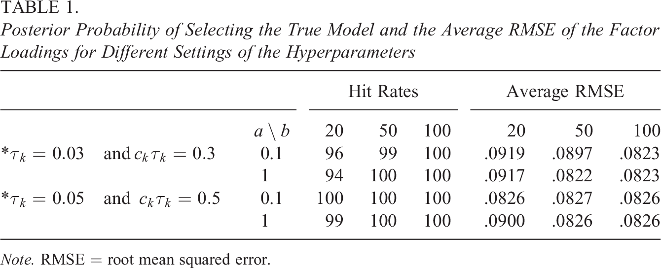
Note. RMSE = root mean squared error.

Table 2 presents the bias (bias) and root mean squared error (RMSE) of the factor loadings estimates obtained by IDIFA when selecting $τ_{k} = 0.03$ , $c_{k} τ_{k} = 0.3$ , $a = 1$ , and $b = 50$ . The estimates are calculated as the posterior mean of the factor loadings after applying the postprocessing scheme in Papastamoulis and Ntzoufras (2022). The bias and RMSE values suggest that IDIFA satisfactorily recovers the parameter values. Selecting $τ_{k} = 0.03$ , $c_{k} τ_{k} = 0.3$ , $a = 1$ , and $b = 50$ led to the lowest average RMSE across the factor loadings (Table 1), so we implement IDIFA in the following sections with these hyperparameter values unless stated otherwise.

Table 2.

Bias and MSE of the Factor Loadings After Estimating the Parameters With IDIFA

Row	Bias			RMSE
1	−.029	.017	.021	.053	.075	.078
2	.034	−.020	.011	.091	.087	.078
3	−.040	−.063	−.028	.075	.093	.069
4	.035	.021	−.020	.082	.080	.088
5	−.024	.009	.015	.079	.117	.083
6	−.007	−.036	.010	.076	.102	.085
7	−.002	−.000	.002	.072	.074	.072
8	.051	−.021	−.025	.094	.104	.086
9	−.009	−.010	.009	.078	.089	.093
10	.006	.018	−.026	.081	.088	.046

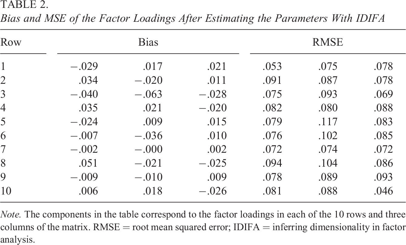
Note. The components in the table correspond to the factor loadings in each of the 10 rows and three columns of the matrix. RMSE = root mean squared error; IDIFA = inferring dimensionality in factor analysis.

BFLS selected the correct number of factors 100/100 times, as well as IDIFA with $τ_{k} = 0.03$ , $c_{k} τ_{k} = 0.3$ , $a = 1$ , and $b = 50$ . However, as illustrated in the following example, when the order of the outcomes is changed and the lower triangular constraint is not adequate to guarantee identifiability, the performance of BF is affected.

Reshuffling the Order of the Outcomes

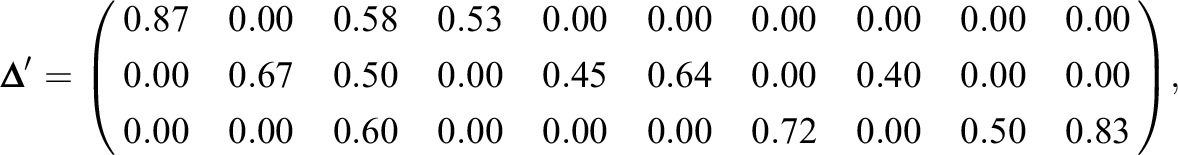
Many simulation studies in the literature, including the above analysis, specify the factor loadings matrix $Δ$ as being positive lower triangular (e.g., Carvalho et al., 2008; Conti et al., 2014; Lopes & West, 2004; Mavridis & Ntzoufras, 2014; Pan et al., 2021). A necessary condition to guarantee identifiability based on the positive lower triangular structure is that the first m rows must be full-rank. In this example, we study the consequences of selecting the number of factors via the BF when this condition is not fulfilled. For this, we repeat the previous simulation study but specifying the factor loadings matrix as

Δ' = (\begin{matrix} 0.58 & 0.87 & 0.53 & 0.00 & 0.00 & 0.00 & 0.00 & 0.00 & 0.00 & 0.00 \\ 0.50 & 0.00 & 0.00 & 0.67 & 0.45 & 0.64 & 0.00 & 0.40 & 0.00 & 0.00 \\ 0.60 & 0.00 & 0.00 & 0.00 & 0.00 & 0.00 & 0.72 & 0.00 & 0.50 & 0.83 \end{matrix}) .

and the idiosyncratic variances are specified as

diag (Σ) = (0.0536,0.2431,0.7191,0.5511,0.7975,0.5904,0.4816,0.8400,0.7500,0.3111) .

This factor loadings matrix and the idiosyncratic variances are the same as in the previous simulation setting, except that the order of the outcomes in the first four positions has changed. For example, the outcome that was in the third position is now in the first one. After this reordering of the outcomes, the first $m = 3$ rows of the factor loadings matrix have rank two, so the positive lower triangular constraint used in BFLS is expected to fail.

After simulating the data, BFLS selected three factors 91/100 times, suggested two factors 3/100 times and selected four factors 7/100 times. In contrast, IDIFA selected the correct number of factors 100/100 times as in the previous simulation setting. As pointed out by one of the reviewers, BF operates as a statistical test, whereas IDIFA selects the best-fitting model, so these two methods are not strictly comparable. However, we contrast here IDIFA with BF since both alternatives can be used to select model dimensionality in practice.

IDIFA does not impose any structure on the factor loadings matrix, so it can perform better in selecting model dimensionality when identifiability cannot be guaranteed based on the positive lower triangular constraint for $Δ$ . Notice that this constraint is generally assumed in Bayesian exploratory factor analysis (e.g., Carvalho et al., 2008; Conti et al., 2014; Lopes & West, 2004; Mavridis & Ntzoufras, 2014; Pan et al., 2021).

As illustrated here, reshuffling the order of the variables in the original data can result in a rank-deficit submatrix in the leading m rows, which causes the positive lower triangular constraint to fail to guarantee identifiability. As a practical implication, the number of selected factors may differ depending on the ordering of the outcomes if the method assumes a lower triangular structure such as BF and most of the methods in the literature for Bayesian factor analysis. When selecting the number of factors with these methods, the choice of the first outcomes is a key modeling decision and not a simple task (Carvalho et al., 2008), but it can be avoided if IDIFA is employed.

Variable Selection on Factor Loadings Components

As discussed in the Introduction, a number of approaches have been proposed to infer model dimensionality assigning a spike-slab prior to the factor loadings $δ_{j k}$ in Equation 1 (see, e.g., Lucas et al., 2006; Carvalho et al., 2008; Conti et al., 2014; Ročková & George, 2016; Chen, 2021) . In this simulation study, we analyze the effect of doing this compared to the IDIFA approach, where the spike-slab is assigned to the parameter $ν_{k}$ in Equation 5, which multiplies the full column of factor loadings.

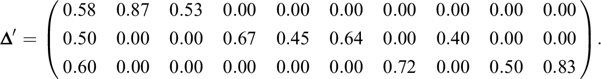
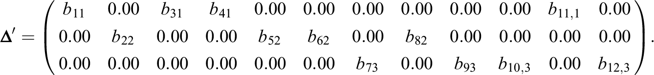
We compare the performance of IDIFA with the proposal in Conti et al. (2014), which is implemented in the R library BayesFM, and also with the BREFA by Chen (2021), which is available in the R package LAWBL. For this, we generate the factor loadings matrix according to the following structure:

Δ^{'} = (\begin{matrix} b_{11} & 0.00 & b_{31} & b_{41} & 0.00 & 0.00 & 0.00 & 0.00 & 0.00 & 0.00 & b_{11, 1} & 0.00 \\ 0.00 & b_{22} & 0.00 & 0.00 & b_{52} & b_{62} & 0.00 & b_{82} & 0.00 & 0.00 & 0.00 & 0.00 \\ 0.00 & 0.00 & 0.00 & 0.00 & 0.00 & 0.00 & b_{73} & 0.00 & b_{93} & b_{10, 3} & 0.00 & b_{12, 3} \end{matrix}) .

The nonzero loadings are randomly generated from a uniform distribution on $[0.5, 0.8]$ . Similarly as in IDIFA, the other two methods select the model dimensionality based on the posterior distribution of the number of factors across MCMC iterations. Taking $m = 4$ , the method in Conti et al. (2014) selects the correct model 94/100 times, whereas BREFA indicates the presence of three underlying factors 93/100 times. Alternatively, the IDIFA approach chooses the correct dimensionality 98/100 times, showing higher power to detect the underlying factors under this scenario. Since some of the results are close to each other, the differences could be due to random chance. Therefore, the simulation was repeated using 1,000 Monte Carlo replications to have more precise results. The conclusions were similar as shown in Table 3.

Table 3.

Percentage of Times That Each Number of Factors Was Selected Using 1,000 Monte Carlo Replications

	One Factor	Two Factors	Three Factors	Four Factors
Conti	.000	.076	.924	.000
BREFA	.002	.083	.915	.000
IDIFA	.000	.006	.979	.015

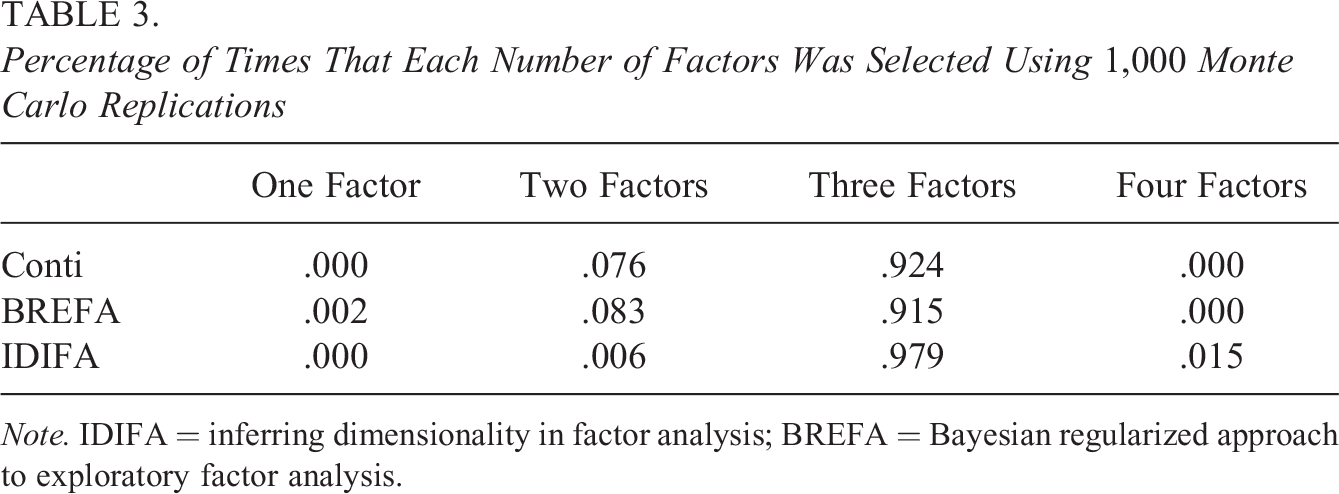
Note. IDIFA = inferring dimensionality in factor analysis; BREFA = Bayesian regularized approach to exploratory factor analysis.

In IDIFA, there is only one indicator $γ_{k}$ for each column of the factor loadings matrix, so the information of the full column is used to decide whether the factor is important in the model. On the other hand, methods such as Conti et al. (2014) and Chen (2021) base the inference on a larger number of indicators $γ_{j k}$ ( $j = 1, \dots, p; k = 1, \dots, m$ ). Therefore, the information in each column is split across outcomes $j = 1, \dots, p$ in order to determine model dimensionality.

A Correlated Factor Model

The model in Equation 1 assumes that the factors are uncorrelated. However, any model with a finite number of factors can be rotated to an orthogonal structure. Indeed, the covariance matrix of the factors can be expressed as $Var (η) = Γ Φ Φ^{'} Γ$ using a variant of the Cholesky decomposition, where $Γ$ is a diagonal matrix with elements proportional to standard deviations of the factors and $Φ$ is a lower triangular matrix that relates to the correlation among the factors. Then, the covariance matrix of the outcomes in Equation 2 is

Ω = Δ (Γ Φ Φ^{'} Γ) Δ^{'} + Σ = (Δ Γ Φ) (Δ Γ Φ)^{'} + Σ,

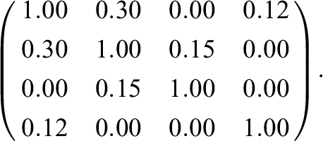
which is equivalent to a model with orthogonal factors and factor loadings matrix $Δ Γ Φ$ . To assess the performance of IDIFA in situations with correlated factors, we simulated a scenario with $p = 16$ outcomes, which are explained by four factors. The first four outcomes are explained by the first factor, whereas the outcomes between number five and eight are explained by the second factor, and so on, so each factor is related to four outcomes. The nonzero factor loadings are generated as $δ_{j k} = (- {1)}^{ϕ_{j k}} \sqrt{a_{j k}}$ , where $ϕ_{j k}$ ~ Ber( 0.5) and $a_{j k} \sim U (0.04, 0.64)$ , whereas the idiosyncratic variances are generated as $σ_{j}^{2} \sim U (0.2, 0.8)$ . The factors are simulated with the following covariance matrix:

(\begin{matrix} 1.00 & 0.30 & 0.00 & 0.12 \\ 0.30 & 1.00 & 0.15 & 0.00 \\ 0.00 & 0.15 & 1.00 & 0.00 \\ 0.12 & 0.00 & 0.00 & 1.00 \end{matrix}) .

The number of observations for this simulation is $n = 400$ and the number of potential factors is $m = 5$ . After generating 100 simulated data sets, IDIFA selected the correct number of factors in all cases demonstrating that the method can work adequately in situations with correlated factors such as in this simulation scenario.

Data Analysis

In the following, we apply the IDIFA approach to two real data sets. First, we use scores on nine mental ability test scores from two different schools in Chicago. In the second data set, we explore the factor structure underlying the measurement of socioeconomic status of students in Colombia. We used three chains with a burn-in of 5,000 iterations, followed by 10,000 additional iterations thinned by a factor of $10$ , which results in a final MCMC sample size of 1,000 for each chain. Relevant code in R and JAGS is provided as Supplementary Material.

The Grant-White School Data Set

In this example, we use scores on nine psychological tests of 301 students in seventh and eighth grades from two different schools (Pasteur and Grant-White) in Chicago. The data are publicly available in the lavaan package (Rosseel, 2012) in R. The data set, first published in Holzinger and Swineford (1939), is used in tutorials to exemplify a three-factor model (Mavridis & Ntzoufras, 2014). Variables 1–3 (visual perception, cubes, and lozenges) are related to “visual perception,” variables 4–6 (paragraph comprehension, sentence completion, and word meaning) are indicators for “verbal ability,” and variables 7–9 (speeded addition, speeded counting of dots, and speeded discrimination straight and curved capitals) relate to “speed.”

Implementing the IDIFA approach with $m = 5$ suggests a three factor model with posterior probability equal to 65%, whereas the four factor model is suggested by 33% of the MCMC iterations and the two factor model is a posteriori supported with probability 2%. Table 4 reports the posterior mean of the factor loadings after applying the postprocessing scheme to the MCMC iterations where $r_{γ} = 3$ . The estimates confirm the hypothesized model, except for variable 9 which loads not only on the second factor but also on the third. These results are similar to those in Papastamoulis and Ntzoufras (2022).

Table 4.

Estimated Posterior Means of Factor Loadings for the Three Factor Model Based on IDIFA for the Grant-White School Data Set

		Factor 1	Factor 2	Factor 3
	Y ₁	−.27	.14	.62
Visual	Y ₂	−.10	−.02	.47
	Y ₃	−.03	.13	.65
	Y ₄	−.82	.10	.17
Verbal	Y ₅	−.85	.09	.09
	Y ₆	−.79	.09	.21
	Y ₇	−.09	.69	−.06
Speed	Y ₈	−.05	.70	.16
	Y ₉	−.13	.50	.40

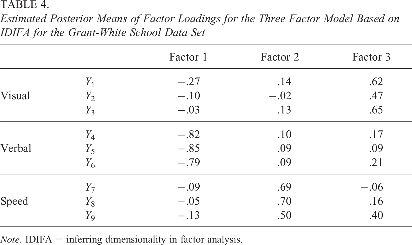
Note. IDIFA = inferring dimensionality in factor analysis.

The convergence of the factor loadings after postprocessing was verified with the BGR diagnostic, the Monte Carlo standard error (MCSE), and the effective sample size (ESS). All values of BGR were smaller than 1.1 and the MCSE was below 5% of the posterior standard deviation of each parameter, indicating convergence in the estimation process (Lesaffre & Lawson, 2012). 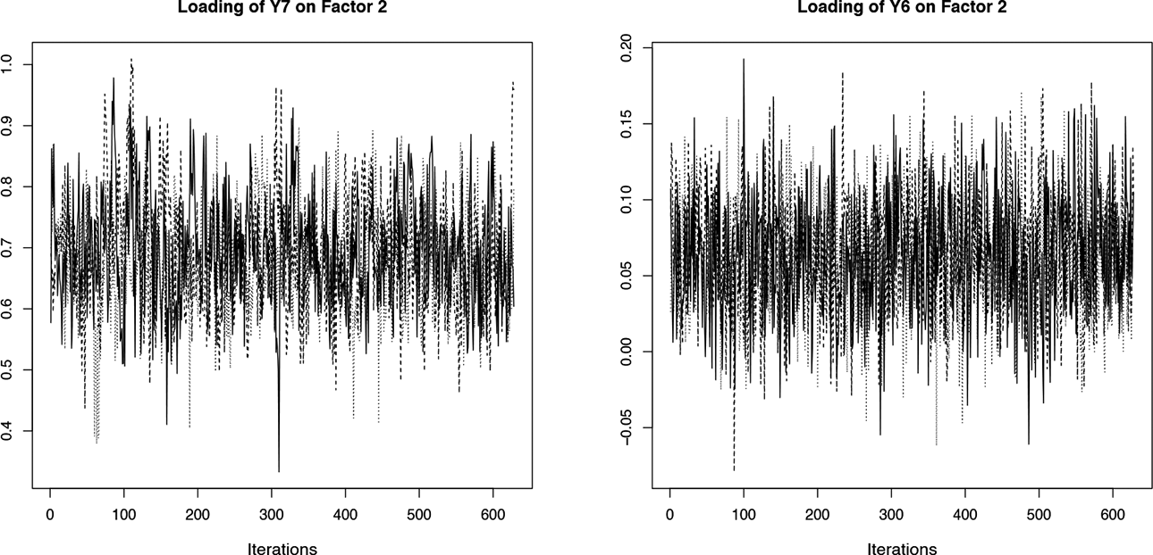The minimum value of ESS was $573$ (loading of Y ₇ on factor 2) and the maximum was $1, 889$ (loading of Y ₆ on factor 2). Figure 2 depicts the traceplot with the three chains for these two loadings and confirms the convergence of the MCMC.

Figure 2.

Traceplot of the factor loadings after applying the postprocessing scheme to the Markov chain Monte Carlo iterations.

Socioeconomic Status of Students in Colombia

We now explore the factor structure underlying the measurement of socioeconomic status of students in Colombia. The cognitive test Saber 11 is administered in the last year of high school. The data set consists of a sample of 235 examinees who answered the test in 2018 in the municipality “El Colegio,” which is near Bogota. A questionnaire was administered to collect eight variables (see Table 5) related to parents’ education attainment (Items 1 and 2), household possessions (Items 3–5), and food consumption at home (Items 6–8). It is of interest to determine whether there are in fact three underlying factors or whether the data could be explained by a unique factor, namely, the socioeconomic status.

Table 5.

Factor Structure for the Items Used in the Measurement of Socioeconomic Status of Students in Colombia Based on a Two Factor Model and a Three Factor Model

	$r_{γ} = 2$		$r_{γ} = 3$
Item	Factor 1	Factor 2	Factor 1	Factor 2	Factor 3
Mother’s education	−.65	.06	.69	.19	.09
Father’s education	−.69	.01	.68	.20	.03
Internet at home	−.46	.24	.22	.64	.07
Number of books at home	−.21	.12	.16	.14	.10
Computer at home	−.47	.35	.20	.70	.18
Milk consumption	−.18	.52	.12	.18	.53
Meat consumption	−.15	.58	.08	.20	.57
Fruit consumption	−.03	.45	.01	.07	.48

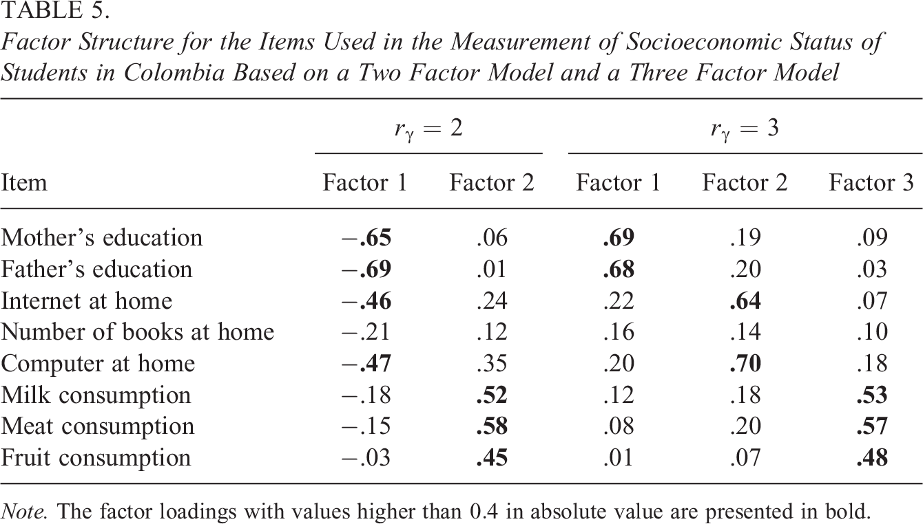
Note. The factor loadings with values higher than $0.4$ in absolute value are presented in bold.

The items related to parental education are ordinal with 10 options between no schooling up to postgraduate studies, while the questions internet at home and computer at home take the values yes/no. The item number of books at home is ordinal with four response options. The questions related to food consumption ask for the number of times the student consumes the item per week and there are four response options lying between almost never and almost everyday.

We implemented IDIFA with $m = 4$ and the results suggest a three-factor structure with a posterior probability equal to 96%. Table 5 reports the posterior mean of the factor loadings after applying the postprocessing scheme in Papastamoulis and Ntzoufras (2022) to the MCMC iterations where $r_{γ} = 3$ . The factor loadings estimates confirm the hypothesized factor structure for all items, except for number of books at home which presents a low factor loading for the household possessions factor. This may be related to the fact that self-reported books in the home by students are subject to endogeneity and systematic errors of observation as discussed in Engzell (2021).

To illustrate what occurs when the maximum number of factors m is lower than the true dimensionality, we carried out again IDIFA but taking $m = 2$ . As a result, the two-factor model is a posteriori supported with probability 100%. Therefore, when the results in IDIFA indicate a probability close or equal to one for $r_{γ} = m$ , it is a signal that the true number of factors may be higher and the value of m should be increased. The solution for the two-factor model groups parental education and household possessions in the first factor (see Table 5 for $r_{γ} = 2$ ), showing that the three-factor solution suggested by IDIFA presents a more reasonable model for the data.

Discussion

Bayesian methods to infer model dimensionality in the literature generally assume a lower triangular structure for the factor loadings matrix. As discussed by Lopes and West (2004), making this assumption before model dimensionality is properly selected may cause that the ordering of the outcomes influences the results. We corroborated this in the simulation study.

In this article, we have proposed an alternative method for Bayesian exploratory factor analysis without imposing any restriction on the factor loadings matrix. In IDIFA approach, we infer model dimensionality based on the number of nonnull columns in the factor loadings matrix. The posterior probability for the selected dimensionality provides information about the certainty/uncertainty on the number of factors given the data. After selecting the number of factors, we solve rotational indeterminacy to estimate the model parameters using the postprocessing scheme in Papastamoulis and Ntzoufras (2022). With respect to the hyperparameter values, selecting $τ_{k} = 0.03$ , $c_{k} τ_{k} = 0.3$ , $a = 1$ , and $b = 50$ performed well in the simulation scenarios and the real data examples.

The Bayesian methods for exploratory factor analysis in the literature base the inference for each column k of the factor loadings matrix on multiple indicators, taking one $γ_{j k}$ for each factor loading $δ_{j k}$ ( $j = 1, \dots, p; k = 1, \dots, m$ ). Using multiple indicators in each column may lead to a loss of power for detecting underlying factors as shown via simulations. In contrast, the IDIFA approach includes one $γ_{k}$ for each factor k and uses the information of the full column in order to determine whether the factor is relevant. Nevertheless, a more comprehensive simulation study is needed to understand more deeply the advantages of IDIFA in terms of power across a wider range of conditions (e.g., nonnormality, more complex structure).

Fitting our model is simple via Gibbs sampling, whereas implementation of the methods in the literature is rather involved in general. This permits that IDIFA can be easily implemented in Bayesian packages. Our proposal assumes that the factors are uncorrelated but may perform well for correlated factor models, since any m-factor model can be rotated to an orthogonal structure.

The model in Equation 4 may be easily extended to analyze hierarchical data by including random effects. Moreover, in cases where one desires to select what outcomes to include in the analysis such as in Kaufmann and Schumacher (2017), a modification of the model in Equation 4 can be implemented. Namely, $y_{i} = N Δ η_{i} + ∊_{i}$ , where $N = diag (ν_{1}, \dots, ν_{p})$ and each component $ν_{j}$ indicates if outcome $j = 1, \dots, p$ is needed in the model. This method is expected to be more powerful to detect important covariates, given that Kaufmann and Schumacher (2017) base the inference on many indicators, taking one $γ_{j k}$ for each factor loading $δ_{j k}$ . Further extensions may be considered to allow for outcomes coming from an exponential family distribution and to deal with missing data.

Supplemental Material

Supplemental Material, sj-docx-1-jeb-10.3102_10769986231176023 - Bayesian Exploratory Factor Analysis via Gibbs Sampling

Supplemental Material, sj-docx-1-jeb-10.3102_10769986231176023 for Bayesian Exploratory Factor Analysis via Gibbs Sampling by Adrian Quintero, Emmanuel Lesaffre and Geert Verbeke in Journal of Educational and Behavioral Statistics

Footnotes

Declaration of Conflicting Interests

The author(s) declared no potential conflicts of interest with respect to the research, authorship, and/or publication of this article.

Funding

The author(s) disclosed receipt of the following financial support for the research and/or authorship of this article: This work was supported by Icfes—Colombian Institute for Educational Evaluation.

ORCID iD

Adrian Quintero

References

Abramowitz

Stegun

I. A.

(1964). Handbook of mathematical functions: With formulas, graphs, and mathematical tables (Vol. 55). Courier Corporation.

Anderson

Rubin

(1956). Statistical inference in factor analysis. In Proceedings of the third berkeley symposium on mathematical statistics and probability, University of California, December, 1954, July and August, 1955 (Vol. 1, p. 111). Held at the statistical laboratory. https://digitalassets.lib.berkeley.edu/math/ucb/text/math_s3_v5_article-08.pdf

Aßmann

Boysen-Hogrefe

Pape

(2016). Bayesian analysis of static and dynamic factor models: An ex-post approach towards the rotation problem. Journal of Econometrics, 192(1), 190–206.

Brooks

S. P.

Gelman

(1998). General methods for monitoring convergence of iterative simulations. Journal of Computational and Graphical Statistics, 7(4), 434–455.

Carvalho

C. M.

Chang

Lucas

J. E.

Nevins

J. R.

Wang

West

(2008). High-dimensional sparse factor modeling: Applications in gene expression genomics. Journal of the American Statistical Association, 103(484), 1438–1456.

Chen

(2021). A Bayesian regularized approach to exploratory factor analysis in one step. Structural Equation Modeling: A Multidisciplinary Journal, 28(4), 518–528.

Conti

Frühwirth-Schnatter

Heckman

J. J.

Piatek

(2014). Bayesian exploratory factor analysis. Journal of Econometrics, 183(1), 31–57.

Dutta

Ghosh

J. K.

(2013). Bayes model selection with path sampling: Factor models and other examples. Statistical Science, 28(1), 95–115.

Engzell

(2021). What do books in the home proxy for? A cautionary tale. Sociological Methods & Research, 50(4), 1487–1514.

10.

Erosheva

E. A.

Curtis

S. M.

(2017). Dealing with reflection invariance in Bayesian factor analysis. Psychometrika, 82, 295–307.

11.

Frühwirth-Schnatter

Lopes

H. F.

(2018). Sparse Bayesian factor analysis when the number of factors is unknown. https://arxiv.org/pdf/1804.04231.pdf

12.

George

E. I.

McCulloch

R. E.

(1993). Variable selection via Gibbs sampling. Journal of the American Statistical Association, 88(423), 881–889.

13.

Geweke

J. F.

Singleton

K. J.

(1980). Interpreting the likelihood ratio statistic in facto models when sample size is small. Journal of the American Statistical Association, 75(369), 133–137.

14.

Ghahramani

Griffiths

T. L.

(2005). Infinite latent feature models and the Indian buffet process. In Advances in neural information processing systems (pp. 475–482). https://papers.nips.cc/paper_files/paper/2005/file/2ef35a8b78b572a47f56846acbeef5d3-Paper.pdf

15.

Ghosh

Dunson

D. B.

(2009). Default prior distributions and efficient posterior computation in Bayesian factor analysis. Journal of Computational and Graphical Statistics, 18(2), 306–320.

16.

Guo

Z. Y.

(2017). Heavy-tailed distributions and risk management of equity market tail events. Journal of Risk and Control, 4(1), 31–41.

17.

Hayashi

Bentler

P. M.

Yuan

K. H.

(2007). On the likelihood ratio test for the number of factors in exploratory factor analysis. Structural Equation Modeling, 14(3), 505–526.

18.

Holzinger

K. J.

Swineford

(1939). A study in factor analysis: The stability of a bi-factor solution. Supplementary Educational Monographs, 48, xi–91.

19.

Kaufmann

Schumacher

(2017). Identifying relevant and irrelevant variables in sparse factor models. Journal of Applied Econometrics, 32(6), 1123–1144.

20.

Kuo

Mallick

(1998). Variable selection for regression models. Sankhyā: The Indian Journal of Statistics, Series B, 60(1), 65–81.

21.

Lee

S. Y.

Song

X. Y.

(2002). Bayesian selection on the number of factors in a factor analysis model. Behaviormetrika, 29(1), 23–39.

22.

Lesaffre

Lawson

A. B.

(2012). Bayesian biostatistics (statistics in practice) (1st ed.). Wiley.

23.

Lopes

H. F.

West

(2004). Bayesian model assessment in factor analysis. Statistica Sinica, 14, 41–67.

24.

Lucas

Carvalho

Wang

Bild

Nevins

J. R.

West

(2006). Sparse statistical modelling in gene expression genomics. Bayesian Inference for Gene Expression and Proteomics, 1, 0–1.

25.

Man

A. X.

Culpepper

S. A.

(2022). A mode-jumping algorithm for Bayesian factor analysis. Journal of the American Statistical Association, 117(537), 277–290.

26.

Mavridis

Ntzoufras

(2014). Stochastic search item selection for factor analytic models. British Journal of Mathematical and Statistical Psychology, 67(2), 284–303.

27.

Mitchell

T. J.

Beauchamp

J. J.

(1988). Bayesian variable selection in linear regression. Journal of the American Statistical Association, 83(404), 1023–1032.

28.

Pan

Wei

Song

(2021). Joint analysis of mixed types of outcomes with latent variables. Statistics in Medicine, 40(5), 1272–1284.

29.

Papastamoulis

Ntzoufras

(2022). On the identifiability of Bayesian factor analytic models. Statistics and Computing, 32(2), 1–29.

30.

Peeters

C. F. W.

(2012). Bayesian exploratory and confirmatory factor analysis: Perspectives on constrained-model selection [Unpublished doctoral dissertation]. Utrecht University.

31.

Ročková

George

E. I.

(2016). Fast Bayesian factor analysis via automatic rotations to sparsity. Journal of the American Statistical Association, 111(516), 1608–1622.

32.

Rosseel

(2012). Lavaan: An r package for structural equation modeling. Journal of Statistical Software, 48, 1–36.

33.

Rowe

D. B.

Press

S. J.

(1994). Bayesian factor analysis by Gibbs sampling and iterated conditional modes.

34.

Simon

M. K.

(2007). Probability distributions involving Gaussian random variables: A handbook for engineers and scientists (1st ed.). Springer-Verlag.

Supplementary Material

Please find the following supplemental material available below.

For Open Access articles published under a Creative Commons License, all supplemental material carries the same license as the article it is associated with.

For non-Open Access articles published, all supplemental material carries a non-exclusive license, and permission requests for re-use of supplemental material or any part of supplemental material shall be sent directly to the copyright owner as specified in the copyright notice associated with the article.

0.00 MB

0.13 MB