
Abstract
Classical automated test assembly (ATA) methods assume fixed and known coefficients for the constraints and the objective function. This hypothesis is not true for the estimates of item response theory parameters, which are crucial elements in test assembly classical models. To account for uncertainty in ATA, we propose a chance-constrained version of the maximin ATA model, which allows maximizing the α-quantile of the sampling distribution of the test information function obtained by applying the bootstrap on the item parameter estimation. A heuristic inspired by the simulated annealing optimization technique is implemented to solve the ATA model. The validity of the proposed approach is empirically demonstrated by a simulation study. The applicability is proven by using the real responses to the Trends in International Mathematics and Science Study (TIMSS) 2015 science test.
In educational measurement, tests should be designed and developed providing evidence of fairness, reliability, and validity (American Educational Research Association et al., 2014). To meet these requirements, a test assembly process should be employed to perform an optimal selection of items from an item bank. In addition to producing test forms that conform to the content and psychometric specifications, a test assembly process ensures that the resulting ability measurements can be trusted and interpreted in a transparent way. Moreover, it can produce comparable measurements in operational settings, where various parallel versions of tests are needed. Furthermore, test assembly plays a crucial role in ability assessment as it lies at the basis of the entire test production process: from the earlier stages of item creation to the selection of items for building the test forms. In detail, the requirements of the final tests specified in the test assembly model not only determine the structure of the test forms but also define the composition of the item pool (Ariel & van der Linden, 2006), guiding the item writing process.
In the last decades, the simplified access to modern digital resources such as sophisticated item banking systems opened the possibility of improving the manual test assembly process through automated test assembly (ATA). The introduction of ATA dramatically improved the quality of the test forms and simplified the test assembly process, especially for large testing programs.
ATA differs from the manual process because the item selection is performed by optimizing mathematical models through specific software called solvers. Automation has brought many advantages over manual test assembly. First of all, a rigorous definition of test specifications reduces the need to repeat some phases of the test development. Secondly, ATA is the only way to find multiple optimal or near-optimal combinations of items starting from large item banks, despite the computational complexity of the task. Thus, ATA is fundamental to making measurements comparable while simultaneously reducing operational costs.
In ATA, mathematical optimization models such as 0–1 linear programming (LP) models (see van der Linden, 2005) are usually applied. These classical models use the item information functions (IIFs) as linear coefficients for the decision variables, which are kept fixed throughout the entire optimization process. However, it is well known that the IIFs are derived from the item parameters estimated within the item response theory (IRT) framework. Consequently, the IIFs should be considered uncertain inputs in the ATA models. Many papers (e.g., Mislevy et al., 1994; Patton et al., 2014; Tsutakawa & Johnson, 1990; Xie, 2019; Zhang et al., 2011; Zheng, 2016) discussed the consequences of uncertainty in item parameters on several aspects of educational measurement, such as the accuracy of ability estimation. However, relatively few studies focused on this issue in the ATA research field. In particular, De Jong et al. (2009), Veldkamp (2013), Veldkamp et al. (2013), Veldkamp and Paap (2017), and Veldkamp and Verschoor (2019) proposed robust alternatives to the classical optimization models. These papers focus on the assembly of single test forms only.
In this article, we propose incorporating the uncertainty in the optimization model for simultaneous multiple test assembly, which is the most applied and discussed ATA model in the literature (Ali & van Rijn, 2016; Debeer et al., 2017; van der Linden, 2005). In more detail, we suggest a test assembly model based on the chance-constrained (CC) approach (see Charnes & Cooper, 1959; Charnes et al., 1958), namely, the CCATA model, by which the
For solving the CCATA model, we developed an algorithm based on simulated annealing (SA), a stochastic meta-heuristic proposed by Goffe (1996). The added value of this technique is represented by the possibility of handling large-sized models, characterized by many optimization variables and constraints, and nonlinear functions. All the proposed algorithms have been coded in the open-source framework Julia (Bezanson et al., 2017) and are free to use as they do not rely on commercial software.
This article is organized as follows. First, the key elements of IRT and ATA are reviewed. The following section discusses the issues arising from uncertainty in IRT and ATA models. Subsequently, an introduction to the CC approach for solving optimization problems with uncertainty is provided. Then, a CC version of the maximin ATA model is proposed. The retrieval of the TIF empirical distribution and the development of a heuristic based on SA for solving the model are discussed in the same section. Afterward, the results of a simulation study are presented in order to compare our proposal to the existing approaches solved by the CPLEX 12.10.0 Optimizer (IBM, 2019). An application of our approach to real data taken from the 2015 TIMSS data is shown. Some concluding remarks and suggestions for applying the CCATA model end this article.
IRT and Test Assembly Models
In educational and psychological measurement, IRT modeling provides several methods to estimate the item parameters. Intending to produce test forms with the highest accuracy in ability estimation, IRT is a solid foundation for ATA methods because the Fisher information function, which is a key object in test assembly, is derived from the item parameter estimates. Given an IRT model, once the items have been calibrated, it is possible to evaluate how informative the test is at various ranges of the latent ability using the TIF, which is defined as the sum of the item Fisher information of all the items in the test (or the inverse of the variance of the maximum likelihood estimator of the ability
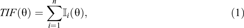
where

The item parameters ai and bi represent the discrimination and the intercept for item i, respectively. 1
From a general point of view, an ATA model is an optimization model consisting of an objective function to be maximized or minimized and a set of constraints to be satisfied. Specific objective functions may be related to psychometric features of the test, such as the maximization of the TIF at given cutoff scores, or to test content or other test requirements, such as the minimization of the total testing time. Examples of constraints include the test length, the restriction on the number of items of a certain type, test overlap, and so on. Altogether, they represent the test specifications, which should be defined in the standard form of Table 1 (van der Linden, 2005, p. 40), before being translated into an ATA model.
Standard Form of a Test Assembly Problem
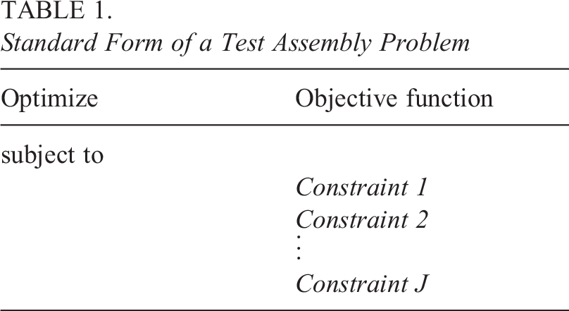
Only one objective can be optimized at a time. If we have more than one function to optimize, some tricks can be applied to transform the objectives into constraints (Veldkamp, 1999), such as the maximin paradigm. On the other hand, there is no upper limit for the number of constraints, provided that the solver can handle the problem (Spaccapanico et al., 2020). If at least one combination of items that meets all the constraints does exist, then the set of these combinations is the feasible set; otherwise, if this set is empty, the model is said to be infeasible. The subset of the feasible set that optimizes the objective function represents the optimal feasible solution.
Tests can be assembled merely through the selection of appropriate items out of an item bank. One way to do so is to use mathematical programming techniques like 0–1 LP or mixed integer programming models and optimize them with commercial solvers, such as
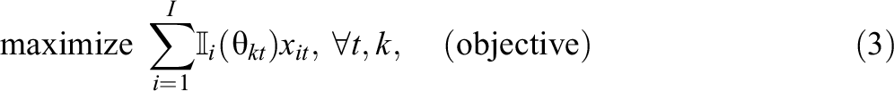
with
Since model (3) has

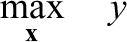
subject to
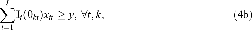

where y is the lower bound for the TIF, so that all the considered TIFs are equal or higher than this value. In this way, the previous objectives are transformed in
In order to describe the structure of the test forms, extra inequalities must often be added to the model due to security concerns. In fact, among others, it may be required to specify a minimum number of items in a given category (e.g., content domain or item type) and the item use among the test forms.
Uncertainty in Test Assembly
In the classical context of test assembly, the optimization models used for item selection do not consider the uncertainty of the estimates of item parameters (van der Linden, 2005). For example, the maximin ATA model is based on the TIF, which appears in the objective function, being the goal of the optimization model. The TIF is the sum of the IIFs of the items in the test form and depends on the item parameter estimates, which are generally considered fixed quantities. Nevertheless, ignoring the uncertainty derived from the estimation process may lead to several issues, such as the misinterpretation of the psychometric properties of the assembled test forms. When the calibration algorithm produces biased estimates for the item parameters, the IIFs are not accurate enough, and, consequently, the TIF of the assembled test might be underestimated or overestimated. In Veldkamp et al. (2013), the authors found that, for large uncertainties, the decrease of information in robust test assembly can reach 37%. As a consequence, the perceived accuracy of ability estimates may be compromised. Mostly regarding the latter issue, a good test assembly model would consider the variation of item parameter estimates in order to build test forms in a conservative manner, that is, it would produce tests with a maximum plausible lower bound of the TIF.
Several attempts to incorporate uncertainty in the test assembly models have been made, mostly by proposing robust approaches. Starting from the conservative approach of Soyster (1973), where the maximum level of uncertainty is considered for 0–1 LP optimization, De Jong et al. (2009) proposed a modified version, where one posterior standard deviation is subtracted from the estimated Fisher information to take the calibration error into account. This approach was also adopted in Veldkamp et al. (2013), where the consequences of ignoring uncertainty in item parameters are studied for ATA models. In addition, Veldkamp (2013) investigated the approach of Bertsimas and Sim (2003), who developed a robust method for LP models by including uncertainty only for some parameters in the assembly of linear test forms. More recently, Veldkamp and Paap (2017) proposed to include the uncertainty related to the violation of the assumption of local independence in ATA for testlets. Finally, Veldkamp and Verschoor (2019) discussed robust alternatives for both ATA and computerized adaptive testing.
The mentioned ATA robust approaches consider the standard error of the estimates and a protection level
A reasonable solution to the mentioned problems appears to be the use of chance-constraints (or probabilistic constraints). In fact, they are among the first extensions proposed in the stochastic programming framework to deal with constraints, where some parameters are uncertain (Charnes & Cooper, 1963; Krokhmal et al., 2002).
Chance-Constrained Modeling
The CC approach (Charnes & Cooper, 1959; Charnes et al., 1958) is a method for optimization problems with uncertainty, where a conservative parameter
More recently, this problem was formulated in terms of percentiles of loss distributions, giving rise to the theory of chance-constraints originally proposed by Charnes and Cooper (1959).
Probabilistic constraints include parameters assumed to be randomly distributed and subject to some predetermined threshold


where
The optimization domain is

where
CC models represent a fully customizable robust approach to optimization. However, although they were proposed in the 1950s, they are still hard to be solved. In fact, a major issue is the general nonconvexity of the probabilistic constraints. Even though the original deterministic constraints
Chance-Constrained Automated Test Assembly
In order to develop a conservative approach that incorporates the uncertainty of item parameters into the ATA model, we propose a stochastic optimization approach for the maximin test assembly model based on the CC method. Under this approach, the TIF is not considered a fixed quantity but a random variable. As explained further on, the distribution of the TIF is retrieved by using the bootstrap technique. Whenever a maximin principle is applied, the CC model can be seen as a percentile optimization problem (Krokhmal et al., 2002). In fact, the probability in the inequality (6) is replaced by the
By considering the maximin model (4a), the constraints (4b) involved in the maximization of the TIF are replaced by the CC equivalents as follows:
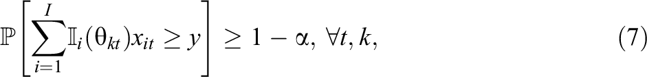
where
The CCATA model maximizes the expected precision of the assembled tests in estimating the latent trait values of the test-takers at the predetermined ability points with a high confidence level if
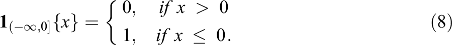
Once the chance-constraints have been defined, a method to compute the probability appearing in inequality (7) should be found. A possible solution is to make assumptions on the probability distribution of
The proposed CCATA model for ATA is based on the empirical distribution of the TIFs of the assembled tests. Therefore, our random variable is the TIF of a test form. This statistic depends on the uncertain IRT item parameter estimates, such as the discrimination and the intercept. There are different ways to retrieve the distribution function of the TIF: Given the standard errors of the estimates, the samples can be uniformly drawn from their confidence intervals as in the robust approach of Veldkamp (2013); otherwise, if a Bayesian estimation is carried out, the samples in the Markov chain can be used.
In this article, another approach is used: A bootstrap procedure is performed to resample the response data and obtain a batch of estimates for each item parameter (see “Empirical Measure of the TIF” section). At the end of this phase, the IIF for all the items in the pool is computed at predefined ability points using the bootstrapped samples. These quantities are then used in the CCATA model to compute the
Empirical Measure of the TIF
The test forms built using the CCATA model should have the maximum possible empirical
Our approach is based on bootstrapping the calibration process. In particular, the observed vectors of responses coming from the full sample (one vector for each test-taker) are resampled with replacement R times, and the item parameters are estimated for each sample. In this way, it is possible to preserve the natural relationship of dependence between the items, and, given the ability targets, it is possible to compute their IIFs. After that, given a set of items, we can build a test form and compute its TIF for each of the R replications. The resulting sample constitutes the empirical distribution function of the TIF.
More formally, let
The Approximated Model
The retrieved empirical distribution function of the TIF is now incorporated into the CCATA model in the following way. Let
Thus, given a specific chance-constraint h, a known set of optimization variables
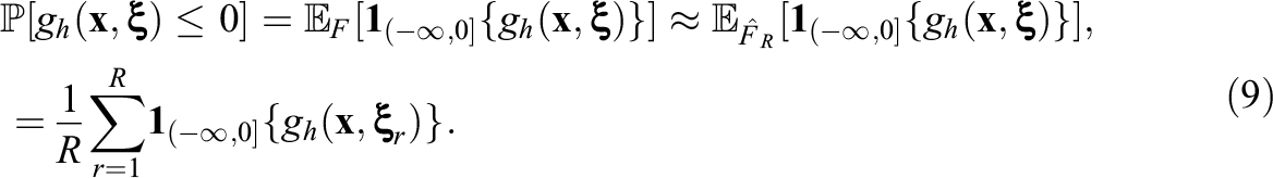
Equation (9) means that the chance-constraint is approximated by the fraction of the R bootstrap samples, in which
Adopting the same principle to the left-hand side of the chance-constraints in inequality (7), the CCATA model can be approximated by

where
The Heuristic
Since a linear formulation cannot effortlessly approximate the proposed CCATA model, a heuristic based on SA (Goffe, 1996) has been developed. This technique can handle large-sized models and nonlinear functions. The theory of SA is derived from the physics of annealing substances. Briefly, we adapted the annealing process to our ATA model by replacing the random selection of a decision variable with the random selection of an item from the item bank. The perturbation of the decision variables is done by adding, removing, or switching the chosen item with another available item. At each modification, the objective function is evaluated and the solution is accepted in accordance with an exponential function based on a parameter called temperature. The higher the temperature, the higher the probability of accepting a worse solution. The temperature is decremented until only better solutions are accepted. The way the temperature is controlled is referred to as the cooling schedule. If there are no further improvements in the area (neighborhood) around the current solution, the process is stopped. At the end, the reannealing phase is actuated if the global stopping criteria have not been reached. In this phase, the best solution obtained is perturbed, the temperature is heated (set to its initial value) and another area is explored. Consequently, more than one neighborhood of the solution space is explored by adopting the SA algorithm, avoiding being trapped in a local optimum. More information about the implementation of the SA algorithm can be found in Spaccapanico (2020) and in the pseudocode in the Appendix.
Unfortunately, the SA algorithm is not able to deal with the constraints, so they are incorporated into the objective function using the hinge function and the Lagrange relaxation, as in Stocking and Swanson (1993). Moreover, the SA has the disadvantage that it can hardly find the feasible space for a problem. Thus, we decided to start our heuristic with a fill up sequential phase: The worst performing test, both in terms of optimality and feasibility, is filled up with the best item available in the item pool. After the selected item has been assigned, the process is repeated until all the tests have reached their maximum length, that is, they are all filled up. Once the first step is performed, we process the solution with the SA principle. The result of the heuristic is a set of solutions with a length equal to the number of neighborhoods explored. Finally, the solution with the best objective function is selected.
Simulation Study
The performance and advantages of the CCATA test assembly model (10) are investigated through a simulation study. Our specific scenario is the on-the-fly test assembly for individualized testing. In fact, we will focus on the average examinee with
All the models are solved using the
The results are compared in terms of the true TIFs averaged across tests and replications. Other benchmarks used to compare the model performances are the relative bias and relative root mean square error (RMSE) between the true and observed TIFs. The true TIF is the reciprocal of the real expected ability estimation error; higher values indicate that the test will produce on average more accurate ability estimates. Moreover, by comparing the values of the relative biases and RMSEs, we can evaluate the accuracy and conservativeness of the models under the specified conditions. In particular, the bias asserts if the observed TIF underestimates (negative values) or overestimates (positive values) the true one. Moreover, as the RMSE approaches zero, the model’s capability to estimate the true TIF increases. On the other hand, high absolute values of the RMSE and bias indicate that the observed TIF is not reproducing the real expected ability estimation error of the test.
Simulation Design
The optimization has been performed on a personal computer with an AMD Ryzen 7 PRO 4750U processor and 16 GB of RAM. Two A pool of For each replication The items are recalibrated The test specifications (see Table 2) are added to the models, and the optimization hyperparameters are set as explained in the next paragraph. For each combination of sample size and set of test specifications, the models
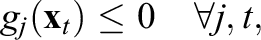
Test Specifications
Performing the bootstrap procedure on the item calibration and solving each ATA model is computationally intensive. In detail, each model requires about 500 seconds to approach its theoretical upper bound of the objective, and the bootstrap procedure takes about 6 to 7 hours, depending on the sample size.
Test Specifications
The mentioned models are solved under different settings, such as the number of test forms and confidence levels. The assembly is performed in a parallel framework, that is, the T tests must meet the same constraints. Two fictitious categorical variables, content_A and content_B, with three possible categories each, are simulated to constrain the tests to have certain content validity. The following specifications replicate realistic ATA applications, where feasibility is the main concern, along with the search for the optimal set of tests in terms of the TIF. The complete set of test specifications is summarized in Table 2.
For example, the constraints described for variable content_A require that tests have 6 to 10 items of the first category of the variable content_A, 9 to 12 items of the second category, and so forth. For classical, 3sd, 1sd, and robust models, different combinations of the specifications in Table 2 create four cases to be investigated in increasing order of complexity. For the CCATA model, eight cases are investigated (four cases for each
Moreover, the hyperparameters for the heuristic are chosen as follows. The starting temperature is equal to 0.1, so the solver does not check solutions too far from the last explored neighborhood, while the geometric cooling parameter is set equal to 0.1. At the beginning of the optimization, we perform one fill up phase, only taking into account the feasibility of the model. Then, we proceed to look for the most optimal combination of items by randomly selecting one item in all the tests to be added, removed, or switched. A Lagrange multiplier equal to 0.1 is chosen to balance the model’s feasibility and optimality. The amount of time needed to solve the model is imposed as the termination criterion, and it is set equal to
Results
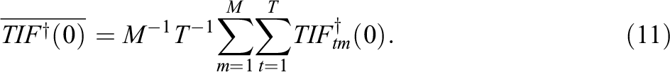
In Table 3 and Figure 1, the mean of the true TIFs computed at
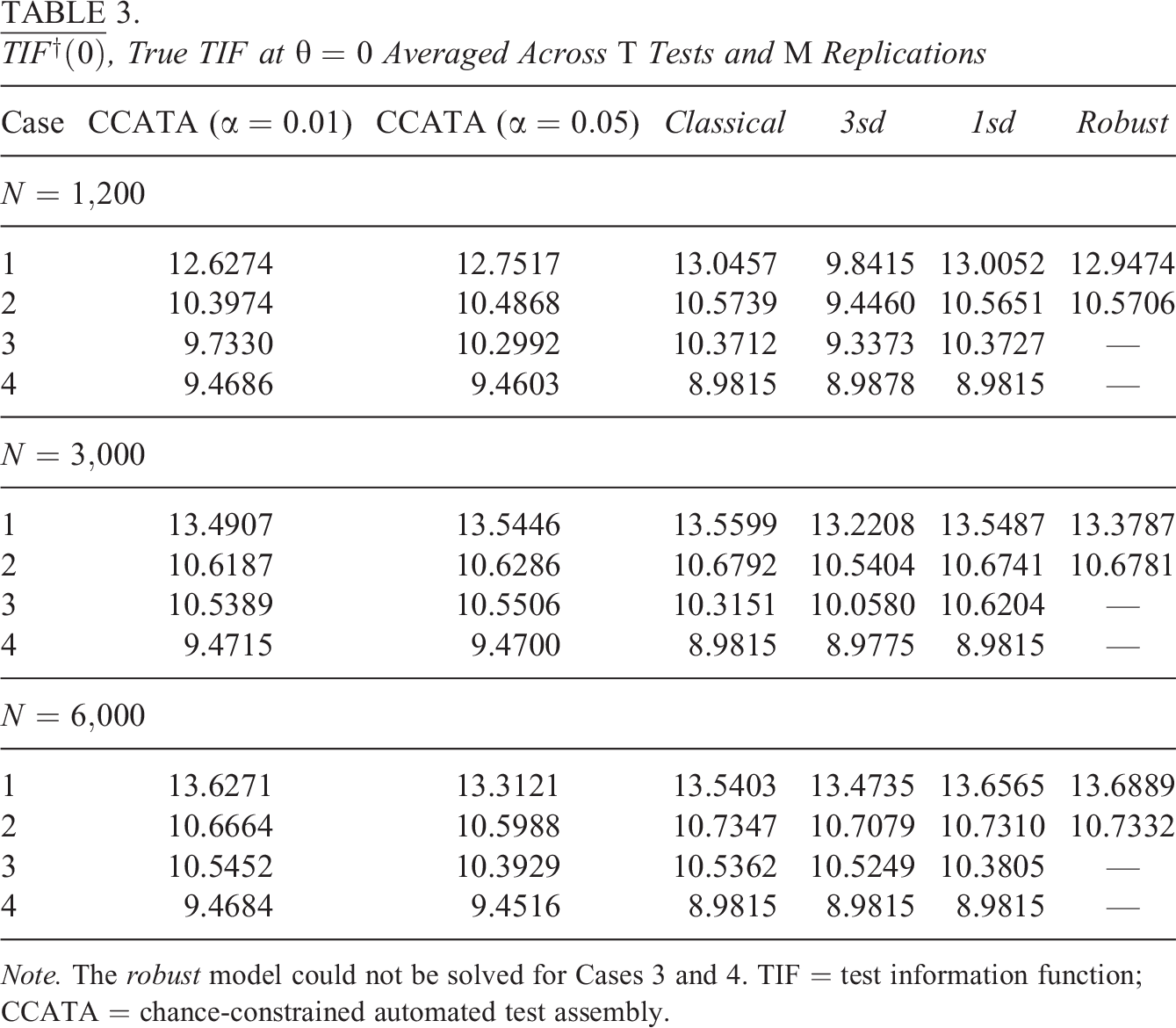
Note. The robust model could not be solved for Cases 3 and 4. TIF = test information function; CCATA = chance-constrained automated test assembly.
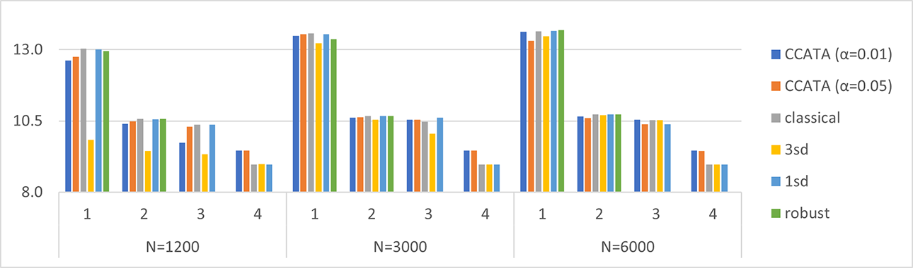
True test information function averaged across tests and replications. Plots are grouped by Case = {1, 2, 3, 4} and by N = {1,200, 3,000, 6,000}.
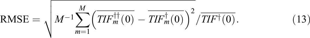
Table 4 and Figure 2 show the results for the relative bias between the observed and true TIF, while Table 5 and Figure 3 for the corresponding relative RMSE. Relative measures are chosen to make the results of the different conditions comparable. The two indicators are obtained as follows. First, for each test t and replication m, the observed TIF,

Relative Bias of the TIF
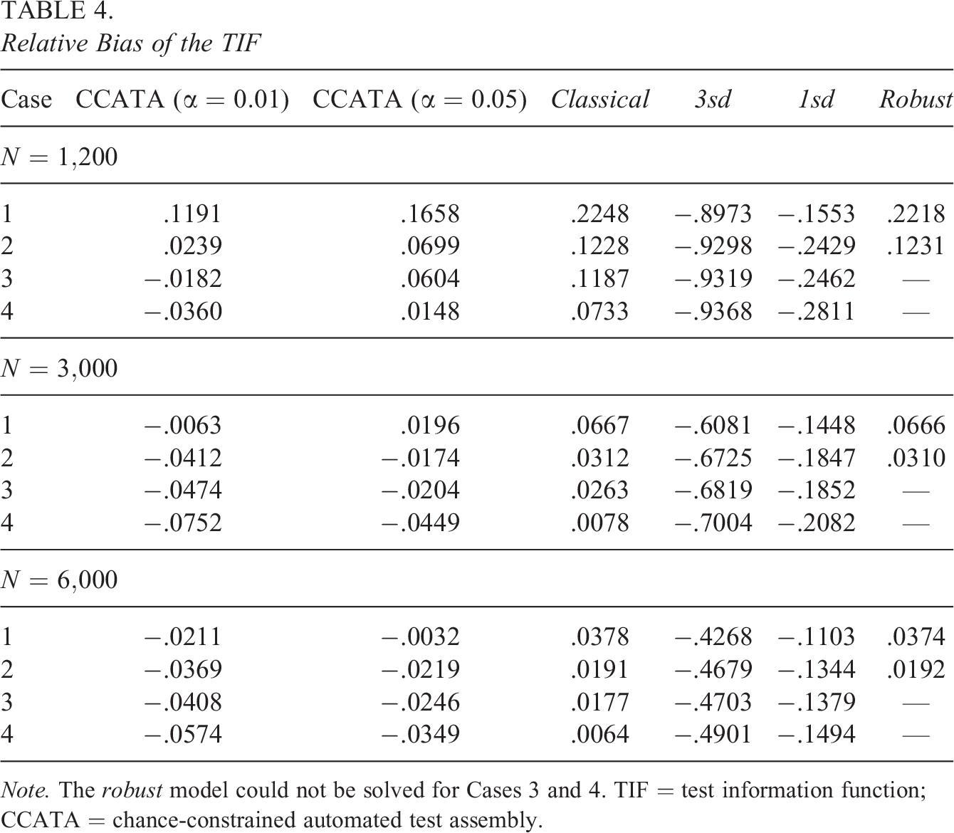
Note. The robust model could not be solved for Cases 3 and 4. TIF = test information function; CCATA = chance-constrained automated test assembly.
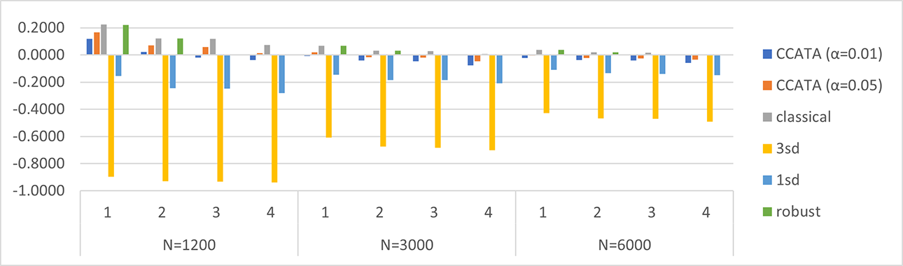
Relative bias of the test information function. Plots are grouped by Case = {1, 2, 3, 4} and by N = {1,200, 3,000, 6,000}.
Relative RMSE of the TIF
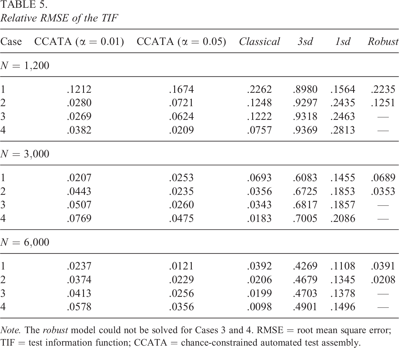
Note. The robust model could not be solved for Cases 3 and 4. RMSE = root mean square error; TIF = test information function; CCATA = chance-constrained automated test assembly.
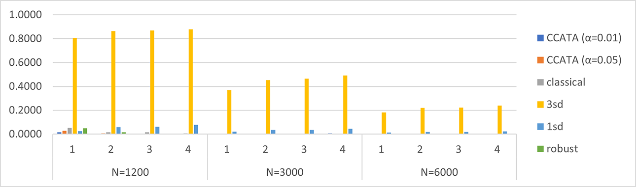
Relative RMSE of the test information function. Plots are grouped by Case = {1, 2, 3, 4} and by N = {1,200, 3,000, 6,000}.
Clearly, the observed TIFs are different for each model. For example, the observed TIF for a particular test under the CCATA model corresponds to the
As can be noticed from Tables 3 through 5, the robust model could not produce any solution under Conditions 3 and 4. These models reached the termination criterion of 500 seconds before a feasible solution was found for all their submodels. For this reason, the robust approach turned out to be impractical for complex, that is, large-sized, ATA models. Specifically, large-sized ATA models are characterized by having several optimization variables and constraints. This condition occurs especially when overlap constraints are imposed, because many auxiliary optimization variables are needed to linearize the model.
Looking at Table 3 and Figure 1, the results on the mean TIF are very similar for all the approaches. However, some patterns have been detected and explained afterward. Lower values of the true TIFs are observed for the 3sd model mainly for the smallest sample size and for
Likewise, the relative biases and RMSEs shown in Tables 4 and 5 and depicted in Figures 2 and 3 are very interesting. As expected, the relative bias and RMSE tend to approach zero as the sample size increases for all the approaches. This behavior is more evident for the classical ATA model. Previous findings about the classical ATA maximin model are confirmed by this simulation. In detail, we observe that the mean TIF obtained with this method overestimates the mean true TIF for all the cases under inspection. The positive bias goes from
The CCATA approach significantly improves the interpretation of the test’s expected precision, which can be expressed as “the tests have a
Application to Real Data
The data used in this application come from the 2015 TIMSS survey, a large-scale standardized student assessment conducted by the International Association for the Evaluation of Educational Achievement. Since 1995, this project has monitored mathematics and science achievement trends in 39 countries every 4 years, in the fourth and eighth grades and in the final year of secondary school. TIMSS 2015 was the sixth of such assessments. Further information regarding this study is available on the TIMSS 2015 Web page. We selected the Italian sample of Grade 8 students for the science test ( four content domains (69 biology items, 57 chemistry items, 58 physics items, and 50 earth science items), three cognitive domains (98 applying items, 88 knowing items, and 48 reasoning items), and four topics (110 items with topic 1, 80 items with topic 2, 33 items with topic 3, and 11 items with topic 4).
Furthermore, a subset of these items is grouped into 27 units.
The design is unbalanced, as students are given only a subset of the items, so missing values appear in the response data. In particular, each item has from 611 to 663 responses. The item parameters were estimated according to the 2PL model. After the calibration, we performed a nonparametric bootstrap with
In the calibrated item pool, the discrimination parameter estimates range from 1e-05 to 4.708, with a mean of 0.920 and a median of 0.867. There are two items with the minimum allowed value of the discrimination estimate. On the other hand, the intercept estimates range from −4.340 to 4.546, with mean and median equal to 0.071 and 0.025, respectively.
The final matrix of the IIFs contains
After we included all the specifications in the model, we ran the optimization algorithm, which implements our heuristic. We selected the same termination criteria as in the simulation study. Before the time limit was reached, the algorithm explored four neighborhoods: The first and the second neighborhoods were not feasible, while the third and fourth neighborhoods produced feasible tests with a minimum
Thus, the best solution is produced within the last neighborhood, where the smallest
TIMSS Data, Features of the Test Forms Assembled by the CCATA Model
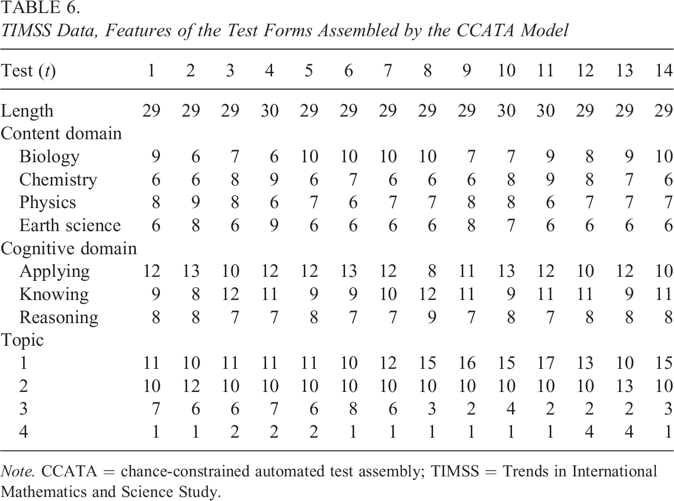
Note. CCATA = chance-constrained automated test assembly; TIMSS = Trends in International Mathematics and Science Study.
The maximized
Test Information Function of the Assembled Tests for TIMSS Data at
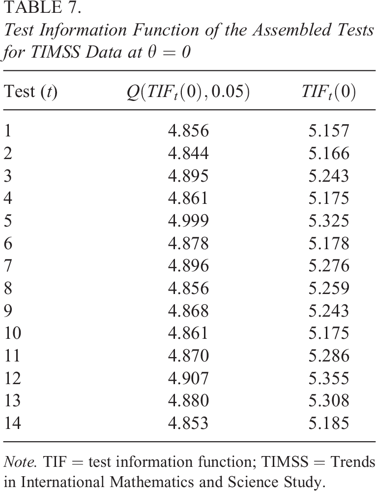
Note. TIF = test information function; TIMSS = Trends in International Mathematics and Science Study.
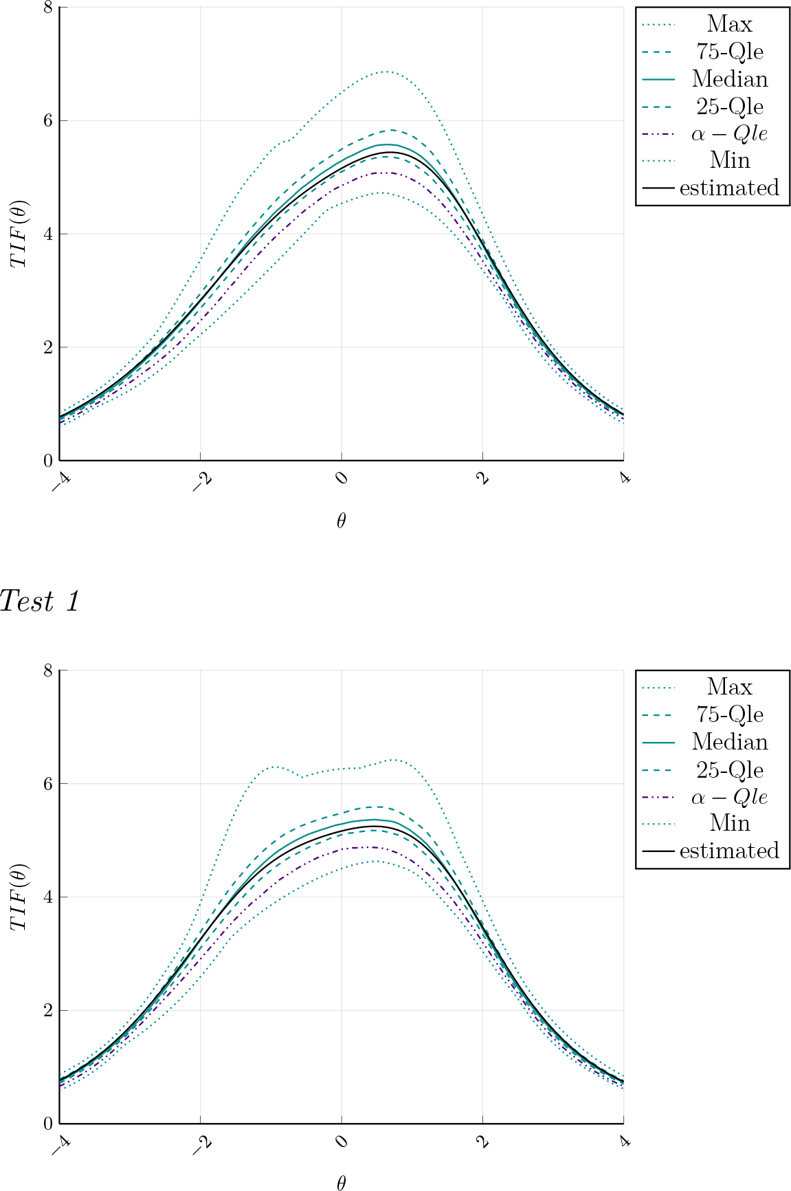
Examples of test information functions (TIFs) of the Assembled Tests 1 and 2. TIF estimated on the full sample (solid black) against quantiles.
The resulting TIFs and quantiles do not considerably differ among the test forms, and this is a signal that the model reached an optimal solution which is very proximal to the global one. However, the high complexity of the model and the low values of the IIFs at
Analyzing the sampling distribution of the TIFs of the assembled tests illustrated in Figure 4, we can notice that the TIF computed on the full sample is consistently higher than the
Concluding Remarks
In this work, a CC version of the maximin ATA model, namely CCATA, has been introduced. This new test assembly model is able to deal with uncertainty in item parameters affected by calibration errors, which, in practice, can be relevant especially for small sample sizes, where the classical approaches highly overestimate the true TIF. In particular, the proposed approach can take into account the structure of the uncertainty observed in the response data used in the calibration phase, with the aim of reducing the risk of misinterpreting the test accuracy in estimating the examinee’s ability. This goal is achieved by approximating the distribution function of the TIF using the bootstrapped replicates of the item parameter estimates. The new model reformulates the classical maximin ATA model in a percentile optimization problem a subcategory of CC models. To deal with the nonlinear formulation of the proposed CCATA model, we developed a heuristic based on the SA principle for finding the optimal conservative tests. In this way, unlike classical and robust optimization techniques, it is also possible to handle large-sized models.
The results of a simulation study in the context of on-the-fly assembly for individualized testing show that the CCATA model, together with our heuristic, maximizes an adjustable conservative version of the TIF, that is, its
The results are encouraging, especially for complex and large-sized ATA models and for small sample sizes. A further contribution to the ATA research field is the development of two open-source
Footnotes
Appendix
Declaration of Conflicting Interests
The author(s) declared no potential conflicts of interest with respect to the research, authorship, and/or publication of this article.
Funding
The author(s) received no financial support for the research, authorship, and/or publication of this article.