
Abstract
Multiple imputation (MI) is a popular method for handling missing data. In education research, it can be challenging to use MI because the data often have a clustered structure that need to be accommodated during MI. Although much research has considered applications of MI in hierarchical data, little is known about its use in cross-classified data, in which observations are clustered in multiple higher-level units simultaneously (e.g., schools and neighborhoods, transitions from primary to secondary schools). In this article, we consider several approaches to MI for cross-classified data (CC-MI), including a novel fully conditional specification approach, a joint modeling approach, and other approaches that are based on single- and two-level MI. In this context, we clarify the conditions that CC-MI methods need to fulfill to provide a suitable treatment of missing data, and we compare the approaches both from a theoretical perspective and in a simulation study. Finally, we illustrate the use of CC-MI in real data and discuss the implications of our findings for research practice.
Keywords
Missing data have received considerable attention in the psychological and educational literature in recent years (e.g., Enders, 2010; Little & Rubin, 2002), and multiple imputation (MI) has become one of the most commonly recommended methods for handling missing data in many areas of research (e.g., Schafer & Graham, 2002). The general idea underlying MI is that missing data are replaced with multiple plausible values that are generated on the basis of the observed data and an imputation model (Rubin, 1987). A key requirement of MI is that the imputation model correctly takes into account the data structure and the relationships between the observed variables. This can be particularly challenging when the data have a clustered structure, in which observations are organized within higher-level units (e.g., students in schools, employees in teams, repeated measures in individuals). Although a number of studies have considered applications of MI in clustered data, much of this research has been concerned with hierarchical data, such as two- and three-level data (Enders et al., 2016; Goldstein et al., 2009; Grund et al., 2018b; Lüdtke et al., 2017; Schafer & Yucel, 2002; Wijesuriya et al., 2020). By contrast, the use of MI applications with nonhierarchical data structures, such as cross-classified or multiple-membership structures, is still poorly understood (for an overview, see Rasbash & Browne, 2008).
The purpose of this article is to investigate the effectiveness of MI for the treatment of missing values in cross-classified data, wherein observations can belong to multiple clusters that do not form a clear hierarchy (Goldstein, 2011; Raudenbush & Bryk, 2002). Cross-classified data are common in many areas of research, for example, in cross-sectional data when individuals are organized in multiple higher-level units (e.g., students in schools and neighborhoods; employees in teams and fields of expertise; see also Claus et al., 2020; Fielding & Goldstein, 2006) or in longitudinal data when cluster membership changes over time (e.g., students in primary and secondary schools; see also Cafri et al., 2015). The treatment of missing data in cross-classified data can be extremely challenging because the variables can be observed at different levels, and the cross-classified structure implies a complex pattern of dependency between the observations that can no longer be captured by hierarchical models.
In writing this article, we have three major goals. First, we aim to clarify the requirements that imputation approaches need to fulfill in order to provide a suitable treatment of missing values in the analysis of cross-classified data. In this context, we focus on analyses with random intercepts and linear effects, and we discuss how the imputation approaches can be extended to address additional types of analyses. Second, we aim to compare the statistical properties of different MI approaches for cross-classified data (CC-MI) from both theoretical and practical perspectives and by using the results of a simulation study. To this end, we (a) introduce a novel approach to CC-MI that is based on the fully conditional specification (FCS) approach to MI and (b) outline a Bayesian joint modeling (JM) approach for the treatment of incomplete cross-classified data. Third, we illustrate the application of CC-MI in a worked example with real data from education research, provide recommendations, and outline limitations and extensions of the approaches that we considered.
This article is organized as follows. In the first section, we provide a brief introduction to the structure and analysis of cross-classified data. In doing so, we try to outline the most important structural features of cross-classified data and explain how they can be analyzed with cross-classified random-effects models (CCRMs). Next, we present the JM and FCS approaches to CC-MI and explain how these methods accommodate the structural properties of cross-classified data. In this context, we also consider ad hoc approaches that extend conventional methods for single- and two-level MI to better accommodate cross-classified data and that can be implemented in a wide variety of statistical software. Then, we present the results of a simulation study, in which we evaluated the statistical properties of these methods. Finally, we demonstrate the application of the methods in an example with computer code and real data, and we discuss the implication of our findings for the treatment of incomplete cross-classified data.
Cross-Classified Data
Cross-classified data are characterized by a clustered structure, in which observations belong to multiple clusters simultaneously. For example, consider the hypothetical scenario in Figure 1, where students are clustered within the units of two random factors: schools (A) and neighborhoods (B). In such a case, students who attend the same school or live in the same neighborhood often tend to be more similar to each other than to students in different schools or neighborhoods because they are exposed to similar contextual influences. Both factors represent higher-level units, and we refer to these levels as Levels A and B. However, in contrast to the clustering that occurs in hierarchical data, the two factors are crossed and not nested within one another. In other words, the students are cross-classified by neighborhoods and schools. This is reflected by the fact that the students at any particular school sometimes live in different neighborhoods, and the students in any particular neighborhood sometimes attend different schools. The combined membership of each student in one school and one neighborhood forms a number of school-neighborhood pairs, in which a certain number of students are nested. We refer to this intermediate level as Level AB. Conceptually, the school-neighborhood pairs may correspond to more tightly knit communities or peer groups that share additional contextual influences that are not shared by other students who attend the same school (but live in different neighborhoods) or live in the same neighborhood (but attend different schools).
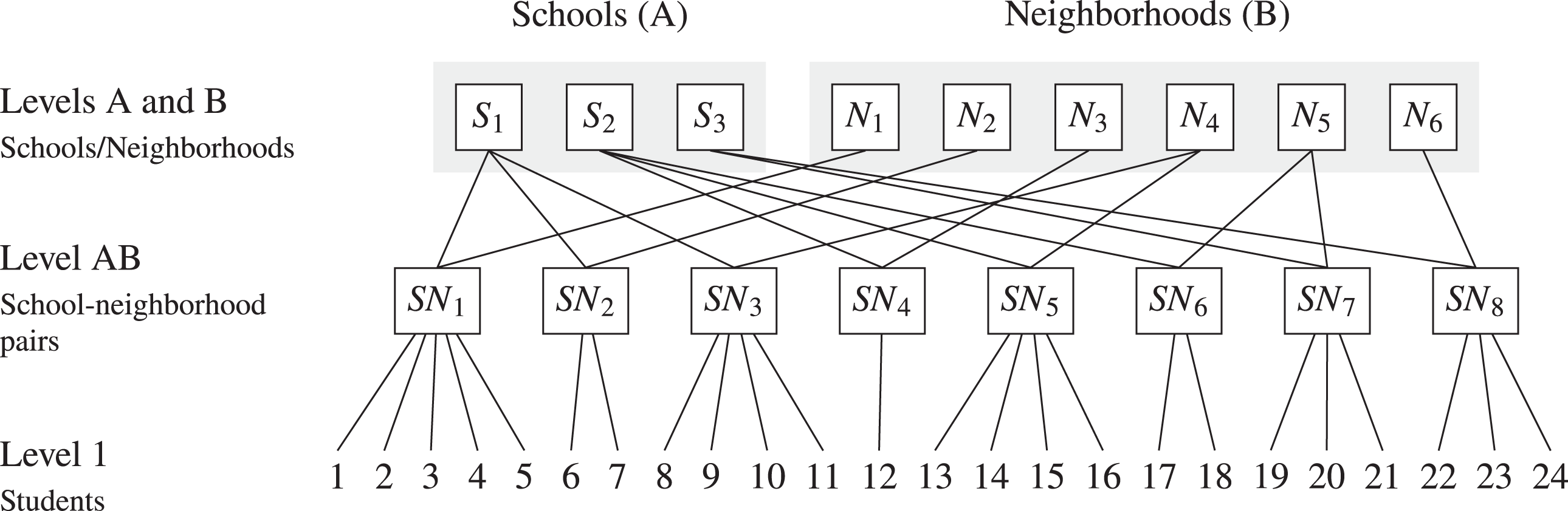
Example of cross-classified data with students (Level 1) clustered in schools (Level A) and neighborhoods (Level B). The two factors (A and B) are crossed, resulting in a number of school-neighborhood pairs (AB), in which the students are nested.
The school-neighborhood assignment shown in Figure 1 is an example of partial cross-classification, in which every school is crossed with only a subset of the neighborhoods and vice versa. The partially cross-classified structure is reflected by the fact that each neighborhood sends students to only some of the schools, and each school recruits students from only some of the neighborhoods. For the example above, the assignment of schools and neighborhoods into school-neighborhood pairs is illustrated in more detail in Figure 2. By contrast, a full cross-classification would occur if every school received students from all the neighborhoods or, equivalently, if every neighborhood sent students to all the schools.
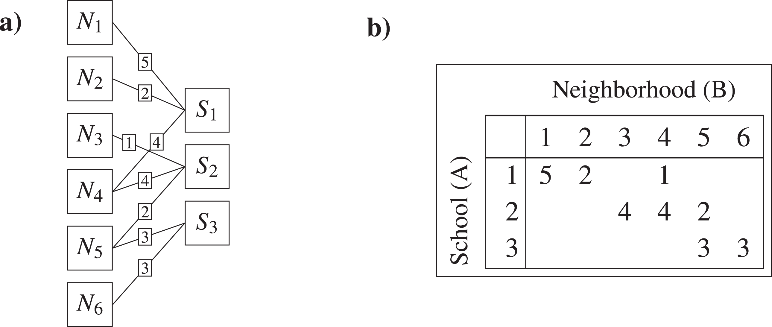
Example (continued) for cross-classified data with students (Level 1) clustered in schools (Level A) and neighborhoods (Level B). The two panels represent the ties between schools and neighborhoods (a) and the number of students for each school-neighborhood pair (b).
Examples of cross-classified data can be found in many areas of research. For example, in education research, cross-classification can occur when schools are crossed with other organizational units, such as neighborhoods or families (e.g., Dundas et al., 2014; Dunn et al., 2015; Garner & Raudenbush, 1991). In longitudinal data, cross-classification occurs when students transition from one type of school to another (e.g., primary and secondary school; Goldstein & Sammons, 1997; Paterson, 1991) or switch classes or teachers over time (e.g., Gregory & Huang, 2013; Heck, 2009; Kyriakides & Creemers, 2008). Finally, cross-classified data can also occur in other areas of research, such as in clinical and organizational research (Barker et al., 2020; Claus et al., 2020), in experimental research (Baayen et al., 2008), or in the context of generalizability theory (Cronbach et al., 1972; Shavelson & Webb, 2000).
Cross-Classified Random-Effects Models
One of the most popular methods for analyzing cross-classified data is the CCRM. Suppose that a researcher is interested in the relationship between an explanatory variable x and an outcome variable y in a sample of students (Level 1) who are clustered within schools (Level A) and neighborhoods (Level B). For example, y may represent students’ academic achievement, whereas x may represent their socioeconomic status (SES).
Intercept-only model
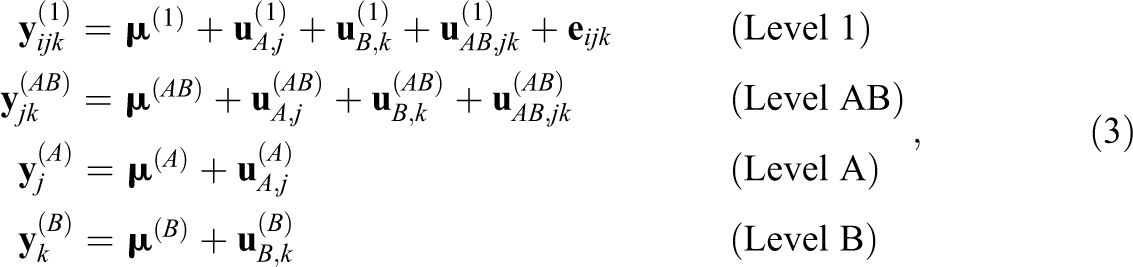
A common first step in the analysis of cross-classified data is to estimate the components of variance in y that can be attributed to differences between schools, neighborhoods, and school-neighborhood pairs, for example, by using the following intercept-only model (Raudenbush & Bryk, 2002). For student i (

where
The main purpose of this model is to distinguish the components of variance in y that pertain to differences between schools (A), neighborhoods (B), and school-neighborhood pairs (
Random-intercept model with explanatory variables
The model above can be extended to address more interesting research questions by including explanatory variables that can be measured at any level of the sample (Raudenbush & Bryk, 2002). In addition, the model can include the cluster means of explanatory variables at Level 1, which allows the effects of this variable to take on different values at different levels. For example, with three explanatory variables x at Level 1, z at Level A, and w at Level B, the model can be extended as follows:

In this model,
Notice that the extended model now partitions both y and x into within- and between-cluster components, although it does so in different ways. Specifically, the components in y are represented by random effects and residuals, whereas the components in x are represented by the values of x at Level 1 (
The models above incorporate the nonhierarchical structure of the data in multiple ways. First, the models include separate random effects and variance components for the two crossed factors A and B. By contrast, if this structure was simplified or ignored, for example, by treating the factors as hierarchical, then the estimated parameters and standard errors could be biased (Lai, 2019; Luo & Kwok, 2009; Meyers & Beretvas, 2006). Second, the models include a random effect of the “interaction” of the two factors, that is, for the combined membership of individuals in a pair of units in A and B. Omitting this component can sometimes simplify the specification of the model but can also induce bias (Shi et al., 2010). As a general rule, including the random effect of the “interaction” requires that there are multiple observations (
Further extensions
The models can also be extended further to address additional research questions. For example, random slopes can be included to allow the effects of the explanatory variables to vary across the units of A or B, and explanatory variables at Levels A or B can be used to explain some of the variance in the slope coefficients (e.g., Raudenbush & Bryk, 2002). In such a model, the effects of lower-level explanatory variables vary both at random and due to the moderating influence of higher-level variables (cross-level interactions [CLIs]). In the following sections, we focus on CCRMs that include only random intercepts and linear effects. We do not consider applications with random slopes, CLIs, or other nonlinear effects in detail, but we return to these extensions later.
MI of Cross-Classified Data
In the following section, we outline two of the main strategies—JM and FCS—that are typically used to conduct MI, and we explain how these strategies can be extended for CC-MI. In addition, we consider a number of ad hoc approaches that are based on imputation approaches for single-level and two-level (hierarchical) data. For simplicity, we focus on applications with continuous data; however, either approach can also be used with categorical data, and we return to this topic in the Discussion section.
Joint Modeling
The general idea underlying the JM approach is that a single (joint) imputation model is specified for all variables with missing data, thus generating imputations for all variables simultaneously. The JM approach was developed primarily in the context of single- and two-level data (Schafer & Olsen, 1998; Schafer & Yucel, 2002; for an overview, see Carpenter & Kenward 2013), but it has also been applied to cross-classified and multiple-membership data (Yucel et al., 2008). To conduct CC-MI with the JM approach, a multivariate CCRM that includes all variables both with and without missing data must be specified.
Suppose that the data comprise observations clustered in two factors A and B as before and with variables measured at different levels. Let further
where
Similar to the univariate intercept-only model in Equation 1, the joint model partitions the within- and between-cluster components in the variables at each level. In addition, the model incorporates the associations that can exist between the components at each level by allowing the random effects and residuals to be correlated (i.e., through
Markov Chain Monte Carlo (MCMC) algorithm
The JM approach to CC-MI can be implemented with MCMC techniques (Browne, 2009; Browne et al., 2001). In the following, we outline the main steps of a generic MCMC algorithm for the estimation of the model parameters and the imputation of missing data at each level (for additional details, see Rasbash & Browne, 2008). For convenience, we write the data of all units and variables as
Draw
Draw
Draw
Draw
Draw
Draw
Compute the observed-data residuals
Compute the observed-data residuals
Compute the observed-data residuals
Compute the observed-data residuals
Update
Notice that the sampling steps for the random effects (Step 6) and the residuals (Step 7) are performed by conditioning on the random effects and the observed values of other variables at the same level. In doing so, the JM approach incorporates information from other variables into the imputation of missing data, while accounting for the relationships that exist between variables at different levels.
To our knowledge, there is currently no software that implements the JM approach to CC-MI (but see Yucel et al., 2008). However, the required sampling steps can be carried out in general-purpose software for Bayesian data analysis, such as WinBUGS/OpenBUGS (Lunn et al., 2000), JAGS (Plummer, 2017), or Stan (Stan Development Team, 2021). In addition, a simplified version of this model with no random effects or variables at Level AB can be fit with the Bayesian estimation procedure in Mplus (Muthén & Muthén, 2017).
Fully Conditional Specification
As an alternative to the JM approach, the joint distribution of the variables with missing data can be approximated by imputing one variable at a time while iterating over a sequence of univariate imputation models, one for each variable with missing data. This strategy is known as the FCS approach to MI (Raghunathan et al., 2001; van Buuren et al., 2006). In the context of CC-MI, each imputation model is set up in such a way that it (a) partitions the within- and between-cluster components of the respective target variable and (b) includes other variables and their cluster means as predictors to represent the relationships between the variables at each level.
Because the FCS approach iterates along a sequence of imputation models, one for each target variable with missing data, different types of models are required to address variables at different levels. Suppose that

where
For target variables at Levels A, B, and AB, the imputation models take on simpler forms but follow the same strategy by conditioning on the other variables at the same levels as well as the cluster means of lower-level variables. Specifically, for variables at Levels A, B, and AB, the models become:
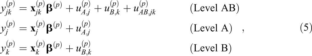
where
Similar to the JM approach, the FCS approach aims to accommodate the cross-classified structure of the data in each imputation model by (a) partitioning the variables in within- and between-cluster components and (b) allowing for associations among the components at different levels. However, in the FCS approach, only the components in the target variables are represented by random effects, whereas those in the predictors are represented by cluster means (see also Enders et al., 2016; Grund et al., 2018b; Lüdtke et al., 2017; Mistler & Enders, 2017). If the cluster means themselves are based on variables with missing data, then they are updated in each step of the procedure, so that they reflect the most recent imputations of the underlying variables (see also Royston, 2005; van Buuren & Groothuis-Oudshoorn, 2011). To our knowledge, the FCS approach to CC-MI is currently supported only by the packages
FCS algorithm
The FCS approach to CC-MI that is implemented in
Update
Fit the model in Equation 4 using the cases with observed data in y to obtain estimates
Draw
Draw
Draw
Draw
Draw
Draw
Notice that the sampling steps for the random effects (Step 4) and the imputations at Level 1 (Step 5) are implemented by conditioning on the predictor variables and their cluster means (in
Single- and two-level FCS with cluster means
As an alternative to CC-MI, cross-classified data can also be accommodated with simpler imputation models (e.g., for single- or two-level data) by including the effects of cluster membership through fixed effects or additional cluster means (Andridge, 2011; Drechsler, 2015; Lüdtke et al., 2017; Wijesuriya et al., 2020). These ad hoc approaches naturally do not offer a full replacement of CC-MI, but they can be useful if software for CC-MI is not available. Here, we consider one such approach that relies on additional cluster means and can be based on single- or two-level FCS.
The FCS approach to CC-MI (Equation 4) accommodates the cross-classified structure of the data by including random effects for the target variable and cluster means for the predictor variables in each imputation model. Cluster means can be included as predictors even in simpler models, so the main difference is how these approaches address the random effects for the target. For example, when using single-level FCS, the random effects for a target variable at Level 1 can be approximated as follows:

where
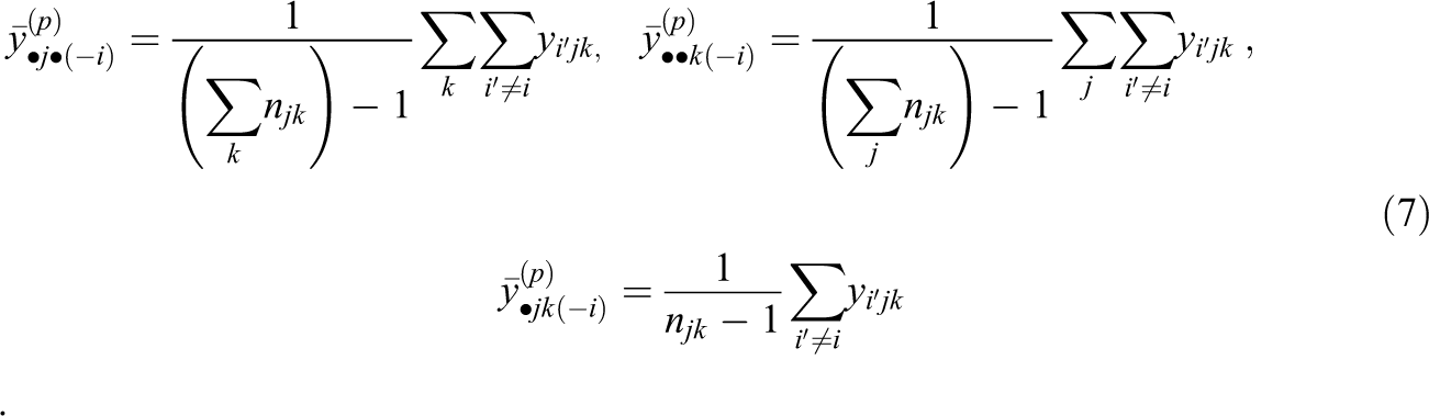
Going forward, we will refer to these cluster means as adjusted cluster means. Conceptually, the adjusted cluster means can be regarded as a proxy for the information about case i that the other cases within the same cluster provide (i.e., the ICC), thus mimicking the contribution of the random effects in CC-MI. This method requires the adjusted cluster means to be updated at each iteration of the imputation procedure with “passive” imputation steps, an option that is provided by many statistical software packages (Raghunathan et al., 2018; Royston, 2005; van Buuren Groothuis-Oudshoorn, 2011).
Differences Between JM and FCS
The main difference between the JM and FCS approaches to CC-MI is how they represent the between-cluster components in the variables included in the imputation model. In the JM approach, the imputation model is based on a multivariate CCRM and represents the between-cluster components with random effects, which correspond to the latent within- and between-group components in the variables at each level (Asparouhov & Muthén, 2006; Lüdtke et al., 2008). By contrast, the FCS approach is based on a sequence of univariate CCRMs, in which the between-cluster components of the target variable are also represented by random effects, whereas those of the predictor variables are represented by manifest cluster means (e.g., Raudenbush & Bryk, 2002).
In the context of hierarchical data, it has been shown that the JM and FCS approaches to MI are equivalent in cases with balanced data, that is, when all clusters have the same size (Carpenter & Kenward, 2013; see also Enders et al., 2016; Lüdtke et al., 2017; Resche-Rigon & White, 2018). Specifically, for balanced data, it can be shown that the two approaches represent the conditional distribution of the missing data in different but equivalent ways, provided that the cluster means are included in the FCS approach. Grund et al. (2018a) further showed that the two approaches provide nearly identical results even in unbalanced data, where the exact equivalence between them no longer holds (see also Resche-Rigon & White, 2018).
In the Appendix, and in more detail in Supplement A in the Online Supplemental Materials, we extend these considerations to cross-classified data and found that the same result holds but under stronger conditions. Specifically, we found that the FCS and JM approaches to CC-MI are asymptotically equivalent in balanced fully cross-classified data, that is, when the number of units in A and B and the cluster sizes are constant and the sample is sufficiently large. The equivalence holds only asymptotically, because the FCS approach induces a slight dependency between marginally independent observations whose strength diminishes as the numbers of units in A and B become large. For this reason, the FCS and JM approaches are not formally equivalent in cross-classified data. Nonetheless, given that the discrepancy between the FCS and JM approaches appears to be relatively minor, we would still expect their performances to be similar in practice (see also Grund et al., 2018a). In addition, from a practical perspective, the FCS approach often has advantages over the JM approach because it allows for a more flexible specification of the imputation models, with finer control over what type of imputation model is used for each variable and which predictor variables are included in them (see also van Buuren et al., 2006).
Previous research on CC-MI has focused primarily on the FCS approach (Wijesuriya, 2021; however, see Yucel et al., 2008) or specific applications, such as missing item responses in educational assessments (Kadengye et al., 2014) or missing data in social network analysis (Jorgensen et al., 2018). In addition, Hill and Goldstein (1998) considered the special case of missing unit identifiers in longitudinally cross-classified data. Overall, these studies suggest that methods for CC-MI can provide an effective treatment of missing values in cross-classified data. However, to our knowledge, no study has systematically compared the JM and FCS approaches to CC-MI in more general settings.
Simulation
In the following, we present the results of a simulation study in which we evaluated the performance of different MI approaches for cross-classified data. This included the JM and FCS approaches to CC-MI as well as ad hoc approaches that were based on single- and two-level MI. The computer code needed to run the simulation study is provided in the OSF repository (https://osf.io/5em2d).
Data Generation
In the simulation study, we generated data for two standardized variables x and y from a multivariate CCRM (see Equation 3) with observations clustered within two crossed factors A (e.g., schools) and B (e.g., neighborhoods). Specifically, for an observation i (

where the random effects (
Partial cross-classification
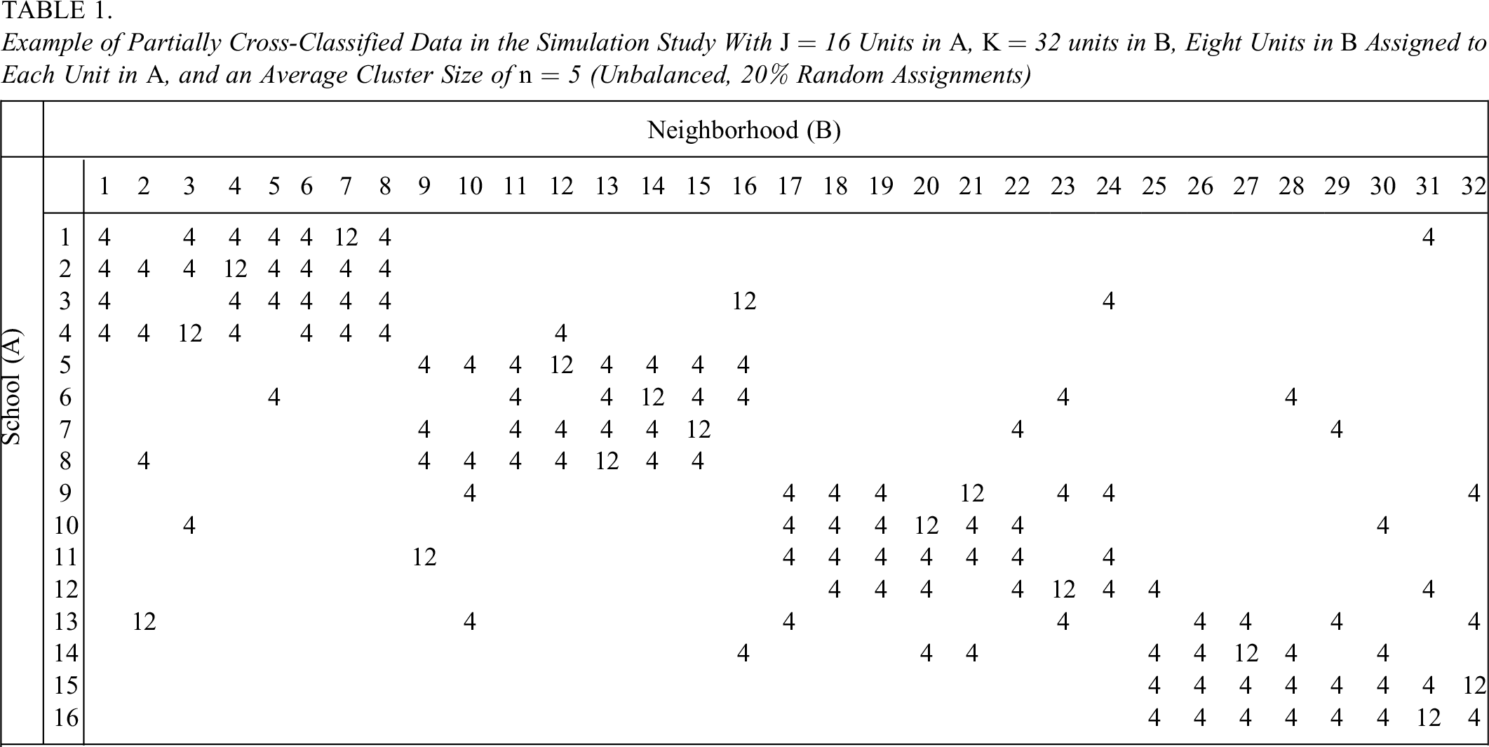
The model in Equation 8 covers both fully and partially cross-classified data. In this study, we focused on partially cross-classified data and used the following procedure to assign a subset of the units in B to a subset of the units in A (see Figure 2). The procedure consisted of two steps. First, we defined the number of units in B that needed to be assigned to each unit in A (
Example of Partially Cross-Classified Data in the Simulation Study With J = 16 Units in A, K = 32 units in B, Eight Units in B Assigned to Each Unit in A, and an Average Cluster Size of n = 5 (Unbalanced, 20% Random Assignments)
Missing data
Once the data were generated, we induced missing values in x on the basis of the values in y in accordance with an missing completely at random (MCAR) or missing at random (MAR) mechanism that we simulated with the following linear model:

In this model,
Simulated Conditions
Using this data generating procedure, we varied the sample sizes at Levels A and B, where we fixed the number of units in A to
Imputation and Analysis
To handle the missing data, we considered 10 different imputation approaches. This included the JM and FCS approaches to CC-MI as well as eight ad hoc approaches based on single- and two-level FCS. The ad hoc approaches included both “naive” specifications of these methods, which reflect common recommendations for applications in single- and two-level data, as well as the extended specifications that aim to accommodate the cross-classified data structure by including adjusted cluster means. Specifically, the methods were as follows:
FCS-1L: single-level FCS.
FCS-1L-M: single-level FCS, extended to include cluster means for the predictor and adjusted cluster means for the target variable (at Levels A, B, and AB).
FCS-2L-A: two-level FCS with random effects of A and cluster means for the predictor.
FCS-2L-A-M: two-level FCS with random effects of A and cluster means for the predictor, extended to include adjusted cluster means for the target variable (at Levels B and AB).
FCS-2L-B: two-level FCS with random effects of B and cluster means for the predictor.
FCS-2L-B-M: two-level FCS with random effects of B and cluster means for the predictor, extended to include adjusted cluster means for the target variable (at Levels A and AB).
FCS-2L-AB: two-level FCS with random effects of
FCS-2L-AB-M: two-level FCS with random effects of
FCS-CC: FCS approach to CC-MI.
JM-CC: JM approach to CC-MI.
To implement JM-CC, we used OpenBUGS (Lunn et al., 2000); and to implement FCS-CC and the methods based on single- and two-level FCS, we used the R packages
In the analysis of the imputed data, we were interested in two different models. The first model was an intercept-only CCRM for x (see Equation 1). The second model was a random-intercept CCRM with y as the outcome variable and x as the explanatory variable (see Equation 2). The parameters of interest were the estimated variance components in x at each level (
Results
The main results are summarized in Tables 2 through 4. For simplicity, we present the detailed results only for selected conditions with
Bias in the Estimated Variance Components for x in Conditions With J = 128 Units in A, K = 128 Units in B, Unbalanced Cluster Sizes, and MAR Data
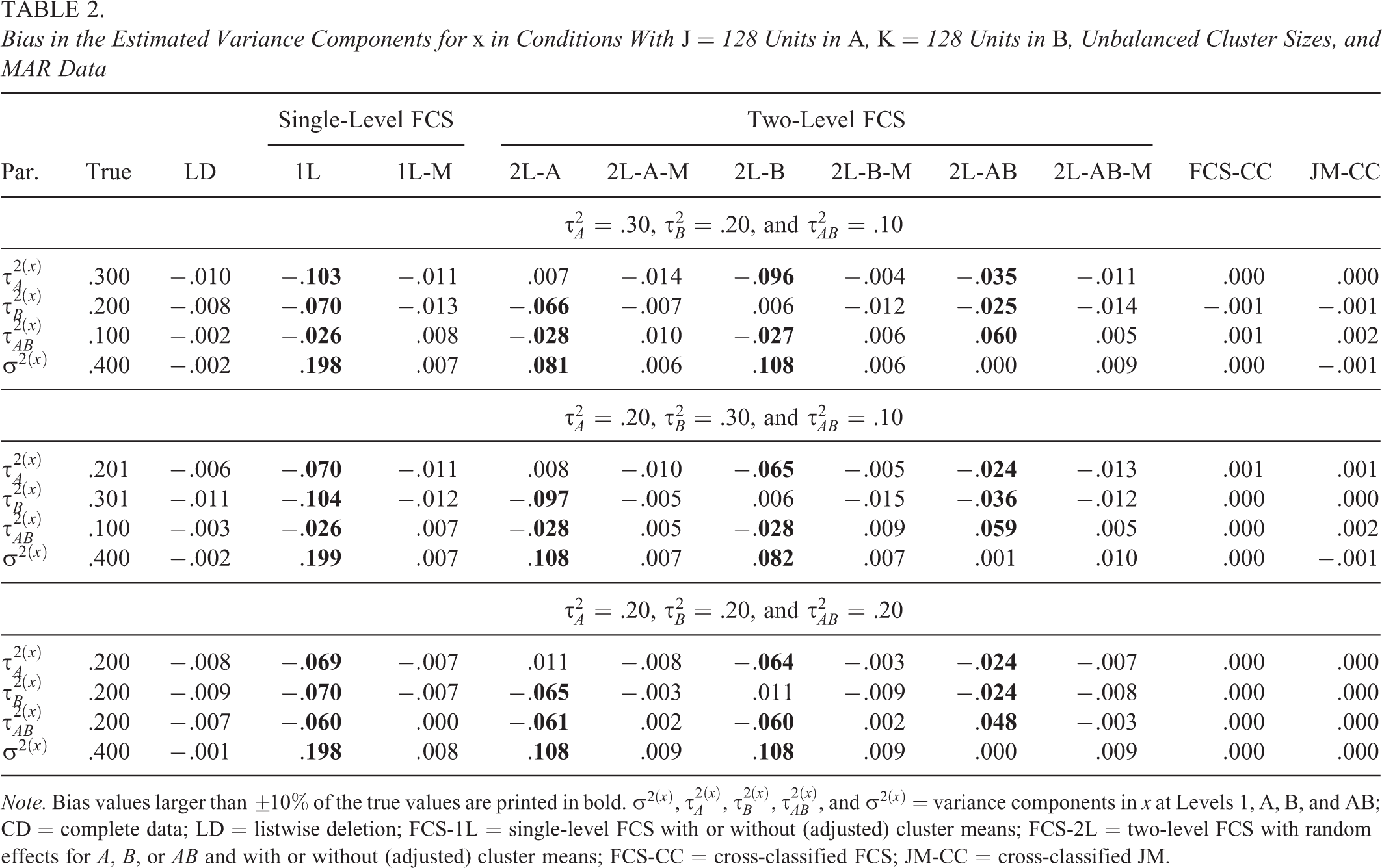
Note. Bias values larger than
The results for the estimated variance components in x are presented in Table 2. The FCS and JM approaches to CC-MI (FCS-CC, JM-CC) provided approximately unbiased parameter estimates in all simulated conditions. By contrast, the single- and two-level FCS approaches (FCS-1L, FCS-2L) led to bias unless their specification was extended to include the adjusted cluster means of the incomplete variable x. The direction and size of the bias depended on the variance configuration and how the random effects at each level were accommodated by these procedures. Specifically, single-level FCS (FCS-1L) underestimated the variances of the random effects and overestimated the residual variance at Level 1. Two-level FCS (FCS-2L-A, FCS-2L-B, and FCS-2L-AB) slightly overestimated the variance of the random effect that was included in the imputation model (e.g.,
The bias in the estimated regression coefficients in the CCRM of y regressed on x is shown in Table 3. Similar to before, FCS-CC and JM-CC provided estimates of the regression coefficients with little to no bias, whereas the estimates provided by the single- and two-level FCS approaches (FCS-1L and FCS-2L) were strongly biased unless their specifications also included the adjusted cluster means of the incomplete variable. When we extended single- and two-level FCS in this manner, the bias in the regression coefficients became smaller for two-level FCS with random effects of A or B (FCS-2L-A-M and FCS-2L-B-M) and even more so for single-level FCS (FCS-1L-M) and two-level FCS with random effects of
Bias in the Estimated Regression Coefficients in the CCRM for y Regressed on x in Conditions With J = 128 Units in A, K = 128 Units in B, Unbalanced Cluster Sizes, and MAR Data
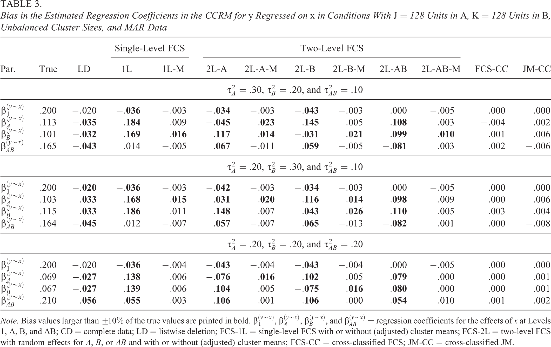
Note. Bias values larger than
Finally, the coverage rates for the 95% CIs of the estimated regression coefficients (Table 4) followed the same pattern as the bias. Specifically, for FCS-CC and JM-CC, the coverage rates were close to the nominal value of 95%. For the single- and two-level FCS approaches without adjusted cluster means (FCS-1L, FCS-2L-A, FCS-2L-B, and FCS-2L-AB), the coverage rates were well below the nominal value. By contrast, when we included the adjusted cluster means, we found coverage rates close to the nominal value for both single- and two-level FCS (FCS-1L-M, FCS-2L-A-M, FCS-2L-B-M, and FCS-2L-AB-M). For LD, we found coverage rates well below the nominal value of 95%. These results were again fairly consistent across conditions, except for LD, which showed nominal coverage under MCAR.
Coverage Rates (%) of the 95% Confidence Intervals for the Regression Coefficients in the CCRM for y Regressed on x in Conditions with J = 128 Units in A, K = 128 Units in B, Unbalanced Cluster Sizes, and MAR Data
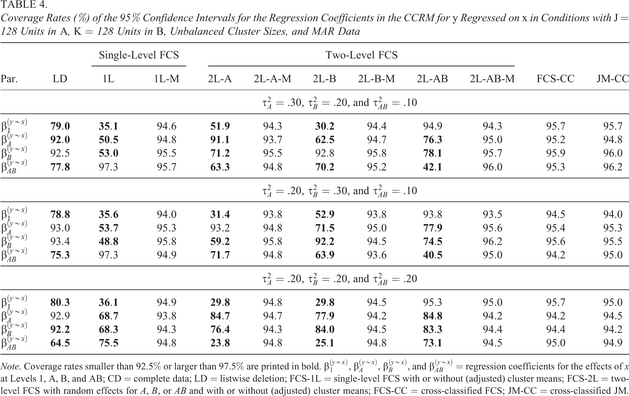
Note. Coverage rates smaller than 92.5% or larger than 97.5% are printed in bold.
To summarize, the results of the simulation study suggested three key findings. First, both the FCS and JM approaches to CC-MI provided accurate results in all simulated conditions. Second, the conventional single- or two-level FCS approaches performed poorly because they failed to accommodate the cross-classified data structure. Third, when the single- and two-level FCS approaches were extended to include the adjusted cluster means for the incomplete target variables, they provided much more accurate results that were very similar to CC-MI. These results are encouraging because they suggest that CC-MI as well as suitable extensions of single- and two-level MI can provide an effective treatment of missing values in cross-classified data.
Example Analysis
To illustrate the application of the different approaches to CC-MI, we use data from the Early Childhood Longitudinal Study (ECLS-K 1998). The ECLS-K is a longitudinal study that focuses on childrens’ early school experiences with multiple measurements beginning in Kindergarten (1998), through primary school (1999–2004), and up to secondary school (8th grade, 2007). An interesting feature of the ECLS-K data is that most children in the sample change schools when they transition from primary to secondary school, which means that the students are cross-classified by primary school (factor P) and secondary school (factor S).
In this example, we use a subset of the ECLS-K data with observations from Grades 5 and 8, comprising a sample of 9,067 students from 1,997 primary and 2,502 secondary schools who changed schools during that time and for whom school membership at both time points was known (Cramér’s V = .858). Specifically, we are interested in the relationship between reading achievement and the amount of time children spent doing homework after their transition to secondary school, controlling for differences between types of schools (private vs. public):

In addition, we fit an intercept-only model for the amount of time spent on homework to quantify the amount of variance between primary schools, secondary schools, and primary-secondary school pairs. In this sample, 553 (6.1%) of the cases had missing data on at least one of the three variables.
To handle the missing data, we used a subset of the methods presented above: LD, single-level FCS with (adjusted) cluster means (FCS-1L-M), and the FCS approach to CC-MI (FCS-CC). These methods were chosen, because they either performed well in our simulation study (FCS-1L-M and FCS-CC) or as a means of comparison (LD). To implement the two MI approaches, we used the R packages
The results are presented in Table 5. Overall, the results showed that students who spent more time on homework had higher reading achievement (at Level 1). In addition, there was a positive contextual effect of time spent on homework at the primary school level (P), indicating that students who had attended primary schools that assigned more homework had higher reading achievement in secondary school. However, there were no contextual effects at the secondary school level (S) or at the level of the primary-secondary school interaction (P-S). There was also a positive effect of the type of school, indicating that students at private (vs. public) schools had higher reading achievement. Finally, the results for the variance components indicated substantial amounts of variance at each level (P, S, and P-S). Due to the relatively small percentage of missing data, the results were very consistent across the methods for handling missing data, and the estimated regression coefficients were usually within half a unit of a standard error from each other. The largest difference in the estimated coefficients was the effect of time spent on homework at the secondary school level, which was essentially zero for LD and slightly positive (but non-significant) for FCS-1L-M and FCS-CC.
Results From the Example Analysis (ECLS-K 1998)
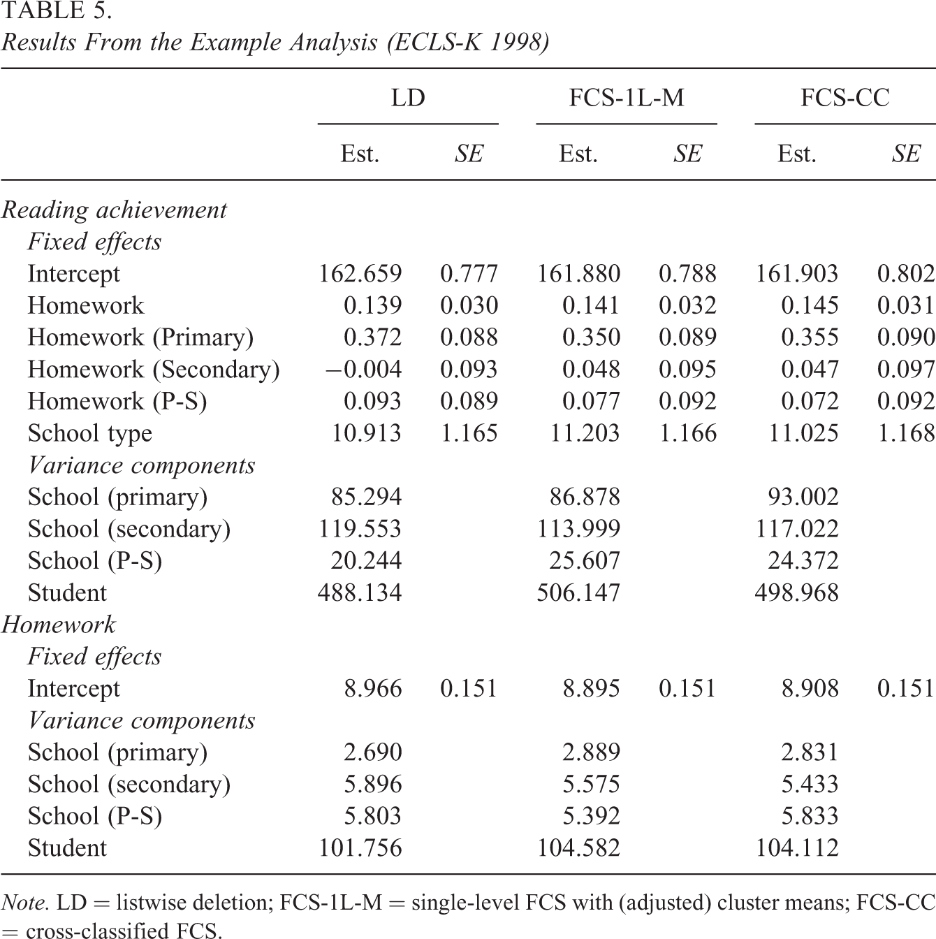
Note. LD = listwise deletion; FCS-1L-M = single-level FCS with (adjusted) cluster means; FCS-CC = cross-classified FCS.
Limitations and Extensions
An important requirement of MI is that the imputation procedure must accommodate the relevant features of the data and the intended analyses. In our study, we focused on applications, in which the intended analyses were CCRMs with random intercepts and explanatory variables with linear effects. For these applications, we outlined how the JM and FCS approaches to MI can be implemented to accommodate cross-classified data, using methods that were either based directly on univariate and multivariate CCRMs (JM-CC and FCS-CC) or that emulated them in an ad-hoc manner (e.g., FCS-1L-M). The main strength of these approaches is that they provide a fairly general treatment of missing data in cross-classified data that support a broad range of CCRMs within these limits. This is particularly useful when the imputed data will be used by multiple analysts and in potentially many different analyses.
Naturally, CCRMs can also be extended by including random slopes or nonlinear effects (e.g., CLIs). These types of effects complicate the treatment of missing data, because they cause conventional MI approaches such as JM and FCS to become incompatible with the intended analysis (Du et al., 2022; see also Seaman et al., 2012). Recent research has shown that substantive-model-compatible (SMC) versions of these approaches can be used to ensure compatibility by including the substantive analysis model directly in the imputation procedure (Bartlett et al., 2015; Goldstein et al., 2014). Several studies have shown that SMC methods can be extremely effective at handling missing data in single- and multilevel analyses with nonlinear effects (Erler et al., 2017; Grund, Lüdtke, et al., 2021; Lüdtke et al., 2020). The main advantage of SMC methods is that they can be fine-tuned to accommodate the more complex features of a particular analysis at the cost of making the treatment of missing data more specific to this analysis.
In principle, SMC versions of the JM and FCS approach to CC-MI could also be used in applications of CCRMs with random slopes and nonlinear effects (see also Goldstein et al., 2014). To our knowledge, there is currently no software that provides SMC versions of JM and FCS for cross-classified data. As an alternative, general-purpose software for Bayesian data analysis (e.g., WinBUGS/OpenBUGS, JAGS, or Stan) can be used to implement an SMC version of JM or the sequential modeling approach (Ibrahim et al., 2002) to MI. The sequential modeling approach ensures compatibility by factorizing the joint distribution of the variables into a sequence of univariate conditional models, one of which corresponds to the intended analysis (Ibrahim et al., 2002; see also Lüdtke et al., 2020).
In addition to the compatibility issues caused by nonlinear effects, it has been shown that the imputation models used in the FCS approach are sometimes incompatible with each other, even if the intended analysis includes only linear effects (Liu et al., 2014; Zhu & Raghunathan, 2015). This issue has also been raised in the context of multilevel analyses, where the conditional models employed by FCS sometimes do not correspond to a well-defined joint model (Resche-Rigon and White, 2018; see also Du et al., 2022). In the present study, we found that a similar problem applies to the FCS approach in cross-classified data (see the Appendix), although this did not have any noticeable impact on its performance (see also Grund et al., 2018a). Nonetheless, the (lack of) compatibility in the FCS approach remains an important issue, and researchers should be mindful when applying this method in practice (for a more detailed discussion, see Du et al., 2022).
Discussion
In the present article, we compared different approaches for the imputation of missing values in cross-classified data (CC-MI). To this end, we introduced an extension of the popular JM and FCS approaches to MI for incomplete cross-classified data. On the basis of theoretical considerations and the results of a simulation study, we found that—though not formally equivalent—both the JM and FCS approaches to CC-MI provided an effective treatment of incomplete cross-classified data. In addition, we found that simpler approaches based on single- or two-level FCS can accommodate cross-classified data by extending the imputation models to include (adjusted) cluster means. Finally, we illustrated the application of these methods with the
Our findings have multiple implications for practice. First, the JM and FCS approaches to CC-MI appear to be similarly suited for handling incomplete cross-classified data. The FCS approach can be particularly convenient because it can easily handle different types of variables (e.g., a mixture of continuous and categorical data) and provides finer control over the selection of predictor variables in each model. For the FCS approach to CC-MI to accommodate the cross-classified structure of the data, the imputation models should include (a) the random effects for each crossed factor and (if possible) their interaction and (b) cluster means of the predictor variables to accommodate the relationships between the variables at each level. As an alternative to CC-MI, cross-classified data can also be handled with simpler techniques that are based on single- or two-level FCS. This can be beneficial when methods for CC-MI are unavailable or suffer from convergence problems. In such cases, single- or two-level FCS approaches can be extended to include (adjusted) cluster means, which can reduce or avoid the computational burden of modeling multiple random effects in CCRMs while providing results that are often similar to CC-MI.
The present study has several limitations in addition to those listed above. First, there are several variants of CCRMs for nonhierarchical data that should be considered in future research. This includes multiple-membership multiple-classification (MMMC) models that can be used to analyze data, in which observations are not only clustered in multiple crossed factors but can also belong to multiple units of the same factor (Browne et al., 2001; Grady & Beretvas, 2010; Park & Beretvas, 2020). Similarly, in longitudinal research, CCRMs can be extended to distinguish between acute and cumulative effects of cluster membership when this membership changes over time (Cafri et al., 2015). Although MMMC and similar models share many of the features of the CCRMs considered in this article, little is known about how multiple-membership structures can and should be accommodated in the treatment of missing data (however, see Yucel et al., 2008). Second, in our simulation study, we focused on partially cross-classified data with structural features that are typical in education research (e.g., Garner & Raudenbush, 1991; Goldstein & Sammons, 1997; Raudenbush, 1993). Future research should also evaluate CC-MI in settings with more challenging features, for example, with a small number of clusters at Levels A and B, or common features from other areas of research, for example, with fully cross-classified data or only a single observation at Level 1 (i.e., without random effects of the “interaction”). Third, we assumed that the identifiers that denote the cluster membership for each unit were fully observed. However, especially in longitudinal data, in which cluster membership can change over time, these identifiers can also be missing, and more research is needed to determine how to handle missing data in these cases (see also Hill & Goldstein, 1998; van Buuren, 2011). Fourth, in our simulation study, we did not consider higher-level variables with missing data (e.g., at Levels A, B, or AB). Future research should therefore evaluate the performance of the different approaches to CC-MI for the treatment of missing data in higher-level variables (see also Enders et al., 2018; Grilli et al., 2022; Grund et al., 2018b). Finally, we evaluated CC-MI only in conditions with MCAR or MAR data. By contrast, when data are missing not at random (MNAR), conducting MI typically requires strong assumptions about the missing data mechanism, which can be evaluated in sensitivity analyses (Carpenter & Kenward, 2013). Future research should therefore evaluate CC-MI in conditions with MNAR data.
To summarize, the present study compared and evaluated multiple approaches to CC-MI, which included both a novel extension of the popular JM and FCS approaches to MI and a number of alternative methods that extend existing methods for single- and two-level MI. We conclude that multiple approaches to CC-MI can provide an effective treatment of incomplete cross-classified data. We hope that the findings presented here motivate further research on statistical methods for handling missing values in cross-classified data and other types of nonhierarchical data.
Supplemental Material
Supplemental Material, sj-pdf-1-jeb-10.3102_10769986231151224 - Handling Missing Data in Cross-Classified Multilevel Analyses: An Evaluation of Different Multiple Imputation Approaches
Supplemental Material, sj-pdf-1-jeb-10.3102_10769986231151224 for Handling Missing Data in Cross-Classified Multilevel Analyses: An Evaluation of Different Multiple Imputation Approaches by Simon Grund, Oliver Lüdtke and Alexander Robitzsch in Journal of Educational and Behavioral Statistics
Footnotes
Appendix
Authors’ Note
Declaration of Conflicting Interests
The author(s) declared no potential conflicts of interest with respect to the research, authorship, and/or publication of this article.
Funding
The author(s) received no financial support for the research, authorship, and/or publication of this article.
Notes
References
Supplementary Material
Please find the following supplemental material available below.
For Open Access articles published under a Creative Commons License, all supplemental material carries the same license as the article it is associated with.
For non-Open Access articles published, all supplemental material carries a non-exclusive license, and permission requests for re-use of supplemental material or any part of supplemental material shall be sent directly to the copyright owner as specified in the copyright notice associated with the article.