Zero and One Inflated Item Response Theory Models for Bounded Continuous Data

Abstract

Bounded continuous data are encountered in many applications of item response theory, including the measurement of mood, personality, and response times and in the analyses of summed item scores. Although different item response theory models exist to analyze such bounded continuous data, most models assume the data to be in an open interval and cannot accommodate data in a closed interval. As a result, ad hoc transformations are needed to prevent scores on the bounds of the observed variables. To motivate the present study, we demonstrate in real and simulated data that this practice of fitting open interval models to closed interval data can majorly affect parameter estimates even in cases with only 5% of the responses on one of the bounds of the observed variables. To address this problem, we propose a zero and one inflated item response theory modeling framework for bounded continuous responses in the closed interval. We illustrate how four existing models for bounded responses from the literature can be accommodated in the framework. The resulting zero and one inflated item response theory models are studied in a simulation study and a real data application to investigate parameter recovery, model fit, and the consequences of fitting the incorrect distribution to the data. We find that neglecting the bounded nature of the data biases parameters and that misspecification of the exact distribution may affect the results depending on the data generating model.

Bounded continuous dependent variables are common in various applications of item response theory (IRT). Examples include the visual analogue scales in the measurement of personality (Ferrando, 2001; Kuhlmann et al., 2017), mood (e.g., Barrows & Thomas, 2018; Cella & Perry, 1986), depression (e.g., Luria, 1975; May & Pridmore, 2020), and quality of life (e.g., Guyatt et al., 1987; Hauser & Walsh, 2008), in which respondents indicate their item response on a line segment. Furthermore, item response times on cognitive test items with item-level deadlines (as advocated by, e.g., Goldhammer [2015]) can be considered bounded continuous responses, and finally, summed dichotomous item scores or ordinal item scores can (pragmatically) be considered as bounded and approximately continuous in some situations (see Dolan, 1994; Rhemtulla et al., 2012).

Similarly as in IRT models for categorical responses, the key of IRT models for bounded continuous responses is to model the expected value of the item response variable for a given person as a function of the underlying person and item parameters. In this article, we focus on bounded IRT models that use a monotonic and S-shaped form for this function. This is similar to the well-known one- and two-parameter logistic models for dichotomous data (Birnbaum, 1968), but it is different from unfolding IRT models (Coombs, 1964; Roberts et al., 2000; see Noel, 2014, for an approach to bounded continuous IRT modeling) that adopt a nonmonotonic form for the response function and censored factor analysis (Muthen, 1989) that adopt a monotonic step function.

One of the first attempts to formulate an IRT model for bounded continuous responses has been by Samejima (1973; see also Ferrando, 2002). Although different special cases exist in this general model, in the most popular and practically feasible special case, the S_B distribution (Johnson, 1949) is assumed for the conditional distribution of the responses. Other bounded IRT models have been proposed based on the beta distribution (Noel & Dauvier, 2007; see also Revuelta et al., 2022, for a related approach in the common factor model), the simplex distribution (Flores et al., 2020), the truncated normal distribution (Müller, 1987), and a distribution based on a truncated exponential function (Verhelst, 2019). In addition, an unbounded normal distribution has been proposed (Ferrando, 2009; Mellenbergh, 1994; Thissen et al., 1983), which is equivalent to the common linear factor model for the continuous responses (Jöreskog, 1971; Spearman, 1904).

This article is motivated by two observations about conventional bounded IRT models: First, interestingly, despite the importance of bounded continuous data in the applications mentioned above, the existing IRT approaches have mostly focused on responses in the open interval (0, 1), but not on responses in the closed interval [0, 1]. Exceptions are the approaches by Verhelst (2019) and Müller (1987) however; unfortunately, these models are challenging to estimate (see Verhelst, 2019) hampering practical applications. As a result, if respondents use the end points of the continuous measurement scale, which—at least in our experience—happens often, the data need to be arbitrarily transformed to prevent the 0 and 1 scores in the dataset to allow the application of bounded IRT models for the open interval (see, e.g., Noel & Dauvier, 2007). We will show below that this practice can majorly affect the parameter estimates of the bounded response model. Second, although there are different models available for bounded continuous responses, due to the lack of a common modeling framework, these models have not been compared directly in terms of parameter recovery, robustness to misspecification, model fit, and real data applications.

Therefore, to address the two issues above, we present a zero and one inflated IRT modeling framework for bounded continuous responses. In this framework, it is straightforward to accommodate the existing bounded IRT models above. In addition, a general Bayesian estimation procedure is proposed to fit and compare the different models. The outline is as follows: First, we review the conventional bounded IRT models and derive a general zero and one inflated approach to accommodate closed interval responses. Next, we show in a real dataset and a simulated dataset that only relatively mild zero or one inflation can already substantially affect the person and item parameter estimates in the conventional bounded IRT models. We then present the Bayesian procedure to estimate the zero and one inflated bounded IRT models and to study model fit. After that, we present the results of two simulation studies to investigate parameter recovery and examine how misspecification of the conditional distribution of the responses affects the modeling results. Finally, we present an application to 22 personality scales to compare the different models empirically. We end with a general discussion.

IRT Models for Bounded Continuous Data

Let $X_{pi}^{\text{'}}\in \left[L,U\right]$ denote the continuous bounded item score of person $p=1,\dots ,N$ to item $i=1,\dots ,n$ that can take values between a theoretical lower bound L and upper bound U. Commonly $L=0$ and $U=100$ in the case of visual analogue scales, $L=0$ and U is equal to the item deadline (e.g., in seconds) in the case of response times and $L=0$ and $U=n$ in the case of summed dichotomous item scores (in the case of 0, 1 scoring). Next, these item scores $X_{pi}^{\text{'}}$ are transformed using $X_{pi}=(X_{pi}^{\text{'}}-L)/ \left(U-L\right)$ , such that $X_{pi}\in \left[0,1\right]$ . As mentioned above, similarly to IRT models for categorical data, IRT models for bounded continuous data focus on $E(X_{pi}|{\text{θ}}_p,{\tau }_i)$ , the expected response of person p on item i conditional on the underlying latent person parameter which is on the real line, that is, ${\text{θ}}_p\in ℛ$ , and the underlying vector of item parameters, ${\tau }_i \in {ℛ}^m$ , where $m$ denotes the number of item parameters in a given model. Commonly, the relation between $E(X_{pi}|{\text{θ}}_p,{\tau }_i)$ and ${\text{θ}}_p$ and ${\tau }_i$ is characterized by an S-shaped function similarly to the well-known one- and two-parameter models for dichotomous data (but see Noel, 2014, for bounded continuous IRT models that adopt nonmonotonic response functions). However, in the one- and two-parameter IRT models, which are based on the Bernoulli distribution, there is only one natural parameter to be modeled, while for bounded continuous IRT models, there are different suitable distributions that commonly include more natural parameters. In the below, we discuss four bounded continuous IRT models mentioned above that are based on different distributions of $X_{pi}$ conditional on ${\text{θ}}_p$ and ${\tau }_i$ : the bounded IRT model based on the S_B distribution for the conditional distribution of $X_{pi}$ (Samejima, 1973), the beta-IRT model (Noel & Dauvier, 2007), the simplex-IRT model (Flores et al., 2020), and the normal-IRT model (Ferrando, 2009; Mellenbergh, 1994; Thissen et al., 1983). We do not consider the models that are based on truncated distributions (Müller, 1987; Verhelst, 2019) because these models are challenging to estimate as mentioned above (although parameter estimation is feasible using pairwise item parameter estimation, see Verhelst, 2019).

S_B-IRT Model

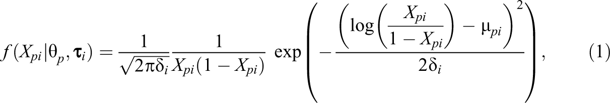
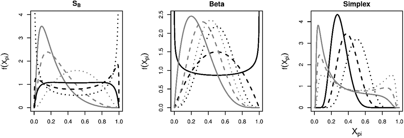
Probably, one of the most well-known models for bounded continuous responses is the model by Samejima (1973). Although the framework outlined by Samejima is much broader, arguably one of the most important special cases (in terms of practical applicability and statistical properties, see Ferrando, 2002) is based on the S_B distribution. The S_B distribution arises if a normally distributed variable, Z, is transformed according to $Z^{\prime }=\psi \left(Z\right)$ , where $\psi (.)$ is the logistic function defined by $\psi \left(d\right)={\left[1+\text{exp}\left(-d\right)\right]}^{-1}.$ See Figure 1 (left) for some example plots of this distribution. If the mean of Z is modeled using a linear IRT parameterization, the following model arises, which we will refer to as the S_B -IRT model:

$f\left(X_{pi}{\text{|θ}}_p,{\tau }_i\right)=\frac{1}{\sqrt{2{\text{πδ}}_i}}\frac{1}{X_{pi}\left(1-X_{pi}\right)}\text{ exp}\left(-\frac{{\left(\text{log}\left(\frac{X_{pi}}{1-X_{pi}}\right)-{\text{μ}}_{pi}\right)}^2}{2{\text{δ}}_i}\right),$

1

with

${\text{μ}}_{pi}={\text{α}}_i{\text{θ}}_p+{\text{β}}_i,$

2

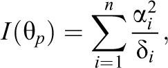
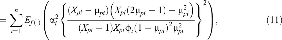
where ${\text{α}}_i\in {ℛ}^{+}$ is an item discrimination parameter on the positive real line, ${\text{β}}_i\in ℛ$ is an item easiness parameter, and ${\text{δ}}_i\in {ℛ}^{+}$ is a dispersion parameter. The expressions for the conditional mean and variance of $X_{pi}$ are complicated and are not provided here (but we refer the reader to the appendix of Johnson [1949]). However, most importantly, $E\left(X_{pi}{\text{|θ}}_p,{\tau }_i\right)$ has a symmetric S-shaped curve with its maximum slope at $E\left(X_{pi}{\text{|θ}}_p,{\tau }_i\right)=\frac{1}{2}$ for ${\text{θ}}_p=-\frac{{\text{β}}_i}{{\text{α}}_i}$ , similarly to the two-parameter model for dichotomous responses (Johnson, 1949; see Ferrando, 2002). In addition, characteristic for this model is that the test information function is constant across ${\text{θ}}_p$ , that is:

$I\left({\text{θ}}_p\right)={\displaystyle \sum }_{i=1}^n\frac{{\text{α}}_i^2}{{\text{δ}}_i},$

while for the IRT models considered next, the test information is not constant across ${\text{θ}}_p$ .

Figure 1.

Examples of the different distributions adopted by the bounded-item response theory models. The parameters used for the S_B distribution for, respectively, the black solid, striped, and dotted lines are: μ = 0,  0.2, 0.1 and δ = 1.5, 2.0, and 3.0 and for the gray solid, striped, and dotted lines: μ = −1.5, −1, and 0 and δ = 1, 1, and 1. In addition, the parameters used for the beta distribution for, respectively, the black solid, striped, and dotted lines are: $\text{a}=\mathit{\text{0.8}}, \mathit{\text{2}},\mathit{\text{ and }} \mathit{\text{4}}$ and $\text{b}=\mathit{\text{0.8}},\mathit{\text{2}}, \mathit{\text{and }}\mathit{4}$ and for the gray solid, striped, and dotted lines: a = 2, 3, and 4 and $\text{b}=\mathit{\text{5}}, \mathit{5}, \mathit{\text{and }}\mathit{5}$ . Finally, the parameters used for the simplex distribution for, respectively, the black solid, striped, and dotted lines are: μ= 0.3, 0.4, and 0.5 and φ = 1, 1, and 1 and for the gray solid, striped, and dotted lines: μ = 0.3, 0.4, and 0.5 and φ = 4, 4, and 4.

Beta-IRT Model

The beta-IRT model (Noel & Dauvier, 2007) assumes a beta distribution for $X_{pi}$ with person and item-specific shape parameters, that is:

$f\left(X_{pi}{\text{|θ}}_p,{\tau }_i\right)=\frac{\text{Γ}\left(a_{pi}+b_{pi}\right)}{\text{Γ}\left(a_{pi}\right)\text{Γ}\left(b_{pi}\right)}{X}_{pi}^{a_{pi}-1}{\left(1-X_{pi}\right)}^{b_{pi}-1},$

3

where $\text{Γ}(.)$ is the gamma function defined by $\text{Γ}\left(d\right)=\underset{0}{\overset{\infty }{{\displaystyle \int }}}{t}^{d-1}\text{exp}\left(-t\right)dt$ and where $a_{pi}\in {ℛ}^{+}$ and $b_{pi}\in {ℛ}^{+}$ . See Figure 1 (middle) for some example plots of this distribution. In the beta-IRT model, $a_{pi}$ and $b_{pi}$ are given by

$a_{pi}=\text{exp}\left(\frac{{\text{α}}_i{\text{θ}}_p+{\text{β}}_i+{\text{ω}}_i}{2}\right),$

4

and

$b_{pi}=\text{exp}\left(\frac{-\left({\text{α}}_i{\text{θ}}_p+{\text{β}}_i\right)+{\text{ω}}_i}{2}\right),$

5

with ${\text{α}}_i$ , ${\text{β}}_i$ , and ${\text{θ}}_p$ defined as before, and with ${\text{ω}}_i\in ℛ$ , so that a dispersion parameter is defined as ${\text{ω}}_i^{\text{'}}=\text{exp}\left(\frac{{\text{ω}}_i}{2}\right)$ . For the beta-IRT model, the conditional mean and variance of $X_{pi}$ are, respectively, given by

$E\left(X_{pi}{\text{|θ}}_p,{\tau }_i\right)=\psi \left({\text{α}}_i{\text{θ}}_p+{\text{β}}_i\right),$

6

and

$VAR\left(X_{pi}{\text{|θ}}_p,{\tau }_i\right)=\frac{E\left(X_{pi}{\text{|θ}}_p,{\tau }_i\right)\left\{1-E\left(X_{pi}{\text{|θ}}_p,{\tau }_i\right)\right\}}{1+2{\text{ω}}_i^{\text{'}}\text{cosh}\left(\frac{{\text{α}}_i{\text{θ}}_p+{\text{β}}_i}{2}\right)},$

where $\psi (.)$ is defined before. Thus, the conditional mean has the same parametric form as the two-parameter logistic model. The original model proposed by Noel and Dauvier (2007) did not contain a discrimination parameter, ${\text{α}}_i$ ; however, we added this parameter to the model to ensure comparability among the different models considered in this study. The test information function for this model is given by

$I\left({\text{θ}}_p\right)=-{\displaystyle \sum }_{i=1}^n{\text{α}}_i^2\left(\text{Ω}\left(a_{pi}+b_{pi}\right){\left(\frac{a_{pi}-b_{pi}}{2}\right)}^2-\text{Ω}\left(a_{pi}\right){\left(\frac{a_{pi}}{2}\right)}^2-\text{Ω}\left(b_{pi}\right){\left(\frac{b_{pi}}{2}\right)}^2\right),$

where $\text{Ω}(.)$ is the trigamma function defined by $\text{Ω}\left(d\right)=\frac{{\partial }^2\text{lnΓ}\left(d\right)}{\partial d^2}$ . Note that this expression differs slightly from that of Noel and Dauvier (2007) as in their model ${\text{α}}_i=1$ . The individual terms in $I\left({\text{θ}}_p\right)$ are the item information functions, which are unimodal functions similar to the item information function in the two-parametric logistic model for dichotomous data with the maximum information at ${\text{α}}_i{\text{θ}}_p+{\text{β}}_i=0$ and with the information about ${\text{θ}}_p$ decreasing as $|{\text{α}}_i{\text{θ}}_p+{\text{β}}_i|$ increases.

Simplex-IRT model

In the simplex-IRT model (Flores et al., 2020), the conditional distribution of $X_{pi}$ is assumed to follow a simplex distribution (Barndorff-Nielsen & Jørgensen, 1991), that is:

$f\left(X_{pi}{\text{|θ}}_p,{\tau }_i\right)=\frac{1}{\sqrt{2\text{π}{\phi }_i{\left[X_{pi}\left(1-X_{pi}\right)\right]}^3}}\text{exp}\left\{-\frac{{\left(X_{pi}-{\text{μ}}_{pi}\right)}^2}{2{\phi }_i{X}_{pi}\left(1-X_{pi}\right){\text{μ}}_{pi}^2{\left(1-{\text{μ}}_{pi}\right)}^2}\right\},$

7

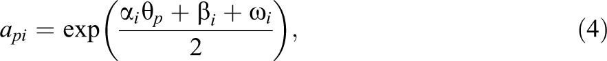
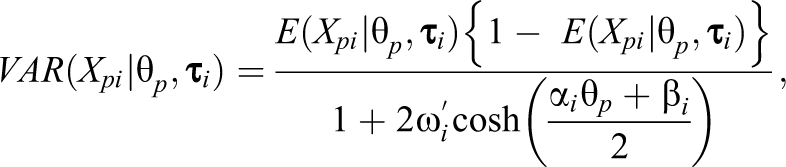
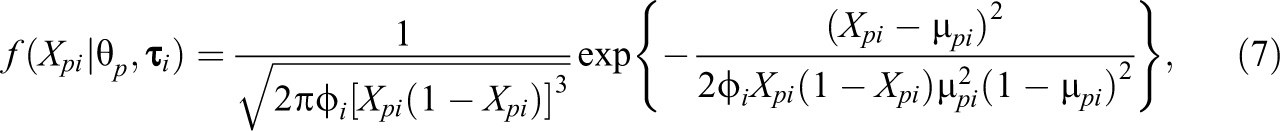
with ${\text{μ}}_{pi}\in \left(0,1\right)$ and with dispersion parameter ${\phi }_i\in {ℛ}^{+}$ . See Figure 1 (right) for some example plots of this distribution. Although relatively less well known as compared to the beta distribution, the simplex distribution has previously been applied in a generalized linear mixed modeling framework to analyze proportions (see Zhang et al., 2016, for applications and an implementation in R). Using the simplex distribution, an IRT model is specified by submitting ${\text{μ}}_{pi}$ to a two-parameter logistic model decomposition (Flores et al., 2020):

${\text{μ}}_{pi}=\psi \left({\text{α}}_i{\text{θ}}_p+{\text{β}}_i\right),$

8

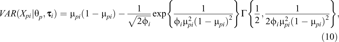
where $\text{ψ}(.)$ , ${\text{α}}_i$ , ${\text{β}}_i$ , and ${\text{θ}}_p$ are defined as before. The conditional mean and variance for the simplex-IRT model are then, respectively, given by

$E\left(X_{pi}{\text{|θ}}_p,{\tau }_i\right)={\text{μ}}_{pi}=\text{ψ}\left({\text{α}}_i{\text{θ}}_p+{\text{β}}_i\right),$

9

and

$VAR\left(X_{pi}{\text{|θ}}_p,{\tau }_i\right)={\text{μ}}_{pi}\left(1-{\text{μ}}_{pi}\right)-\frac{1}{\sqrt{2{\phi }_i}}\text{exp}\left\{\frac{1}{{\phi }_i{\text{μ}}_{pi}^2{\left(1-{\text{μ}}_{pi}\right)}^2}\right\}\text{Γ}\left\{\frac{1}{2},\frac{1}{2{\phi }_i{\text{μ}}_{pi}^2{\left(1-{\text{μ}}_{pi}\right)}^2}\right\},$

10

where $\text{Γ}(.)$ is the upper incomplete gamma function defined by $\text{Γ}\left(x,d\right)=\underset{x}{\overset{\infty }{{\displaystyle \int }}}{t}^{d-1}\text{exp}\left(-t\right)dt$ and where $\text{ψ}(.)$ is defined before.

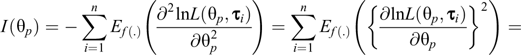
The simplex-IRT model above has originally been proposed by Flores et al (2020) as a measurement model response times. Here, we study the model in the broader context of measurement models for bounded continuous responses. As Flores et al. focused on response times modeling, they did not provide an expression for the test information function. However, it is straightforward to derive, that is:

$I\left({\text{θ}}_p\right)=-{\displaystyle \sum }_{i=1}^n{E}_{f(.)}\left(\frac{{\partial }^2\text{ln}L\left({\text{θ}}_p,{\tau }_i\right)}{\partial {\text{θ}}_p^2}\right)={\displaystyle \sum }_{i=1}^n{E}_{f(.)}\left({\left\{\frac{\partial \text{ln}L\left({\text{θ}}_p,{\tau }_i\right)}{\partial {\text{θ}}_p}\right\}}^2\right)=$

$={\displaystyle \sum }_{i=1}^n{E}_{f(.)}\left({\text{α}}_i^2{\left\{\frac{\left(X_{pi}-{\text{μ}}_{pi}\right)\left(X_{pi}\left(2{\text{μ}}_{pi}-1\right)-{\text{μ}}_{pi}^2\right)}{\left(X_{pi}-1\right)X_{pi}{\phi }_i{\left(1-{\text{μ}}_{pi}\right)}^2{\text{μ}}_{pi}^2}\right\}}^2\right),$

11

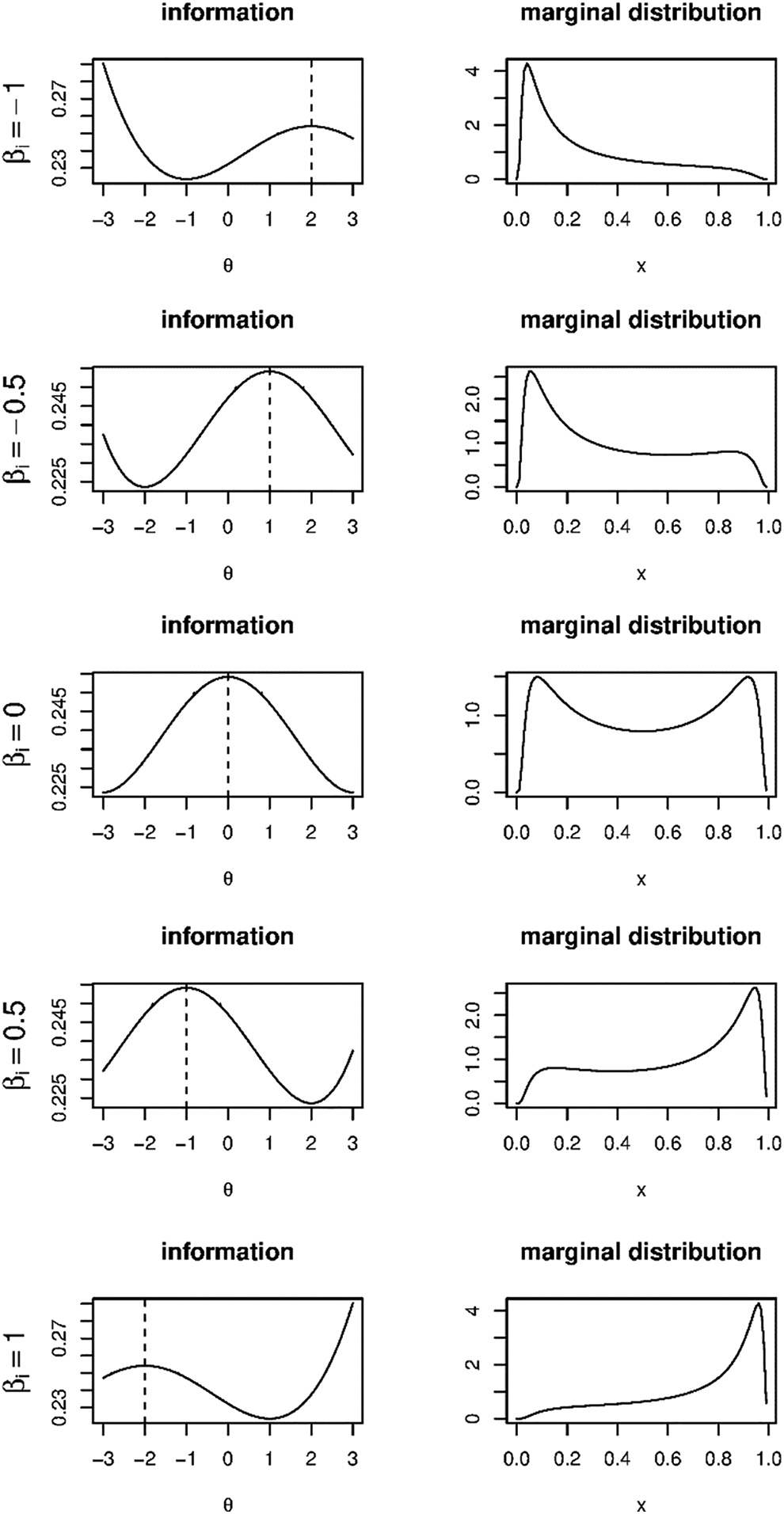
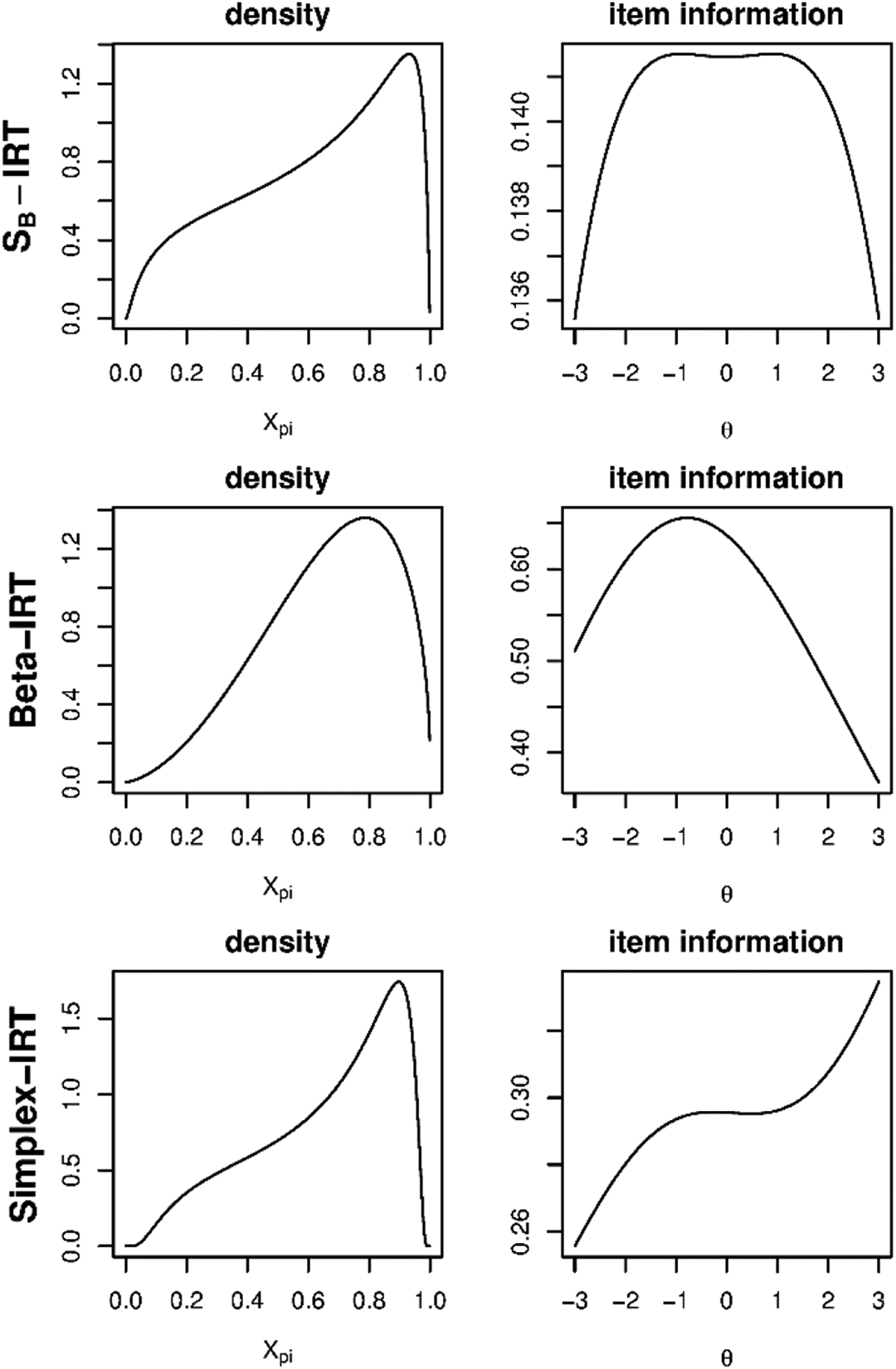
where the expectation is taken in the distribution of $X_{pi}$ , that is, $f(.)$ in Equation 7, ${\text{μ}}_{pi}$ is given by Equation 8, and $lnL\left({\text{θ}}_p,{\tau }_i\right)$ is the log-likelihood function based on Equation 7. The form of the item information functions (i.e., the individual terms in $I\left({\theta }_p\right)$ ) differs importantly from those of the beta-IRT model. That is, for the simplex-IRT model, the item information is increasing toward both ends of the ${\text{θ}}_p$ -scale, whereas for the beta-IRT model, the information is decreasing toward the ends of the ${\text{θ}}_p$ -scale. Similar to the beta-IRT model, however, the item information function of the simplex-IRT model has a maximum at $-{\text{β}}_i/{\text{α}}_i$ . As the simplex-IRT model is not well studied yet and the item and test information functions have not been derived before, we provide some example item information plots in Figure 2. As mentioned in the figure caption, the item information in the simplex-IRT increases to infinity for $\text{θ}\to -\infty$ and $\text{θ}\to \infty$ . This can be verified from Equation 11: In the squared first-order derivative of the log-likelihood with respect to $\text{θ}$ , ${\left(\frac{\partial \text{ln}L\left({\text{θ}}_p,{\tau }_i\right)}{\partial {\text{θ}}_p}\right)}^2$ , it holds that for ${\text{μ}}_{pi}\to 0$ and ${\text{μ}}_{pi}\to 1$ , which happens for $\text{θ}\to -\infty$ and $\text{θ}\to \infty$ , ${\left(\frac{\partial \text{ln}L\left({\text{θ}}_p,{\tau }_i\right)}{\partial {\text{θ}}_p}\right)}^2$ approaches $\infty$ . As a result, the item information also approaches $\infty$ .

In comparing the distributions from the different models in Figure 1, it can be seen that all models can account for bimodality to some degree, which has shown to be relevant in psychological data by Noel (2014). The models still however differ in the exact form of the bimodality, for instance, in the beta distribution, the two modes always occur for $X_{pi}\to 0$ and $X_{pi}\to 1$ , while for the S_B and the simplex distribution, both modes can occur for $0>X_{pi}>1$ .

Figure 2.

Examples of the simplex-item response theory item information function (left column) and the corresponding marginal distributions (right column) for α _i = 0.5, ${\mathit{\text{ϕ}}}_{\text{i}}=15$ , and ${\mathit{\text{β}}}_{\text{i}}$ equal to −1, −0.5, 0, 0.5, or 1. The vertical striped line indicates ${\mathit{\text{θ}}}_{\text{p}}=-{\mathit{\text{β}}}_{\text{i}}/{\mathit{\text{α}}}_{\text{i}}$ . Note that in all situations, the information increases to infinity for θ →−∞ and $\mathit{\text{θ}}\to \infty$ , but this is not visible in all plots.

Normal-IRT Model

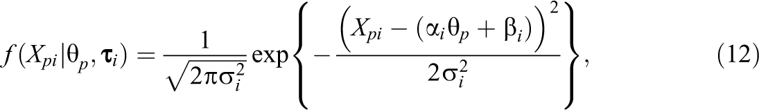
An unbounded normal distribution has also been proposed for bounded continuous data. The main focus of this article is on the bounded IRT models above, but we will also consider the normal-IRT model as a reference to compare the results to. We focus on the parameterization of Mellenbergh (1994) and Thissen et al. (1983), that is:

$f\left(X_{pi}{\text{|θ}}_p,{\tau }_i\right)=\frac{1}{\sqrt{2{\text{πσ}}_i^2}}\text{exp}\left\{-\frac{{\left(X_{pi}-\left({\text{α}}_i{\text{θ}}_p+{\text{β}}_i\right)\right)}^2}{2{\text{σ}}_i^2}\right\},$

12

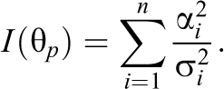
where ${\text{α}}_i$ , ${\text{β}}_i$ , and ${\text{θ}}_p$ are defined as before, and where ${\text{σ}}_i^2\in {ℛ}^{+}$ is a dispersion parameter. The conditional mean and variance of $X_{pi}$ in the normal-IRT model are, respectively, given by ${\text{α}}_i{\text{θ}}_p+{\text{β}}_i$ and ${\text{σ}}^2$ . In addition, similar like the S_B -IRT model, the test information function is constant and given by

$I\left({\text{θ}}_p\right)={\displaystyle \sum }_{i=1}^n\frac{{\text{α}}_i^2}{{\text{σ}}_i^2}.$

Comparability of the Parameters

As the models differ in their formulation, question arises how the parameters can be compared across the models. First, if ${\text{θ}}_p$ is identified in the same way across all models, its estimates can readily be compared. That is, as ${\text{θ}}_p$ is a latent variable, it lacks a scale. By identifying this scale in the same way in all models (e.g., by imposing a Normal(0,1) distribution), ${\text{θ}}_p$ estimates can be compared across models.

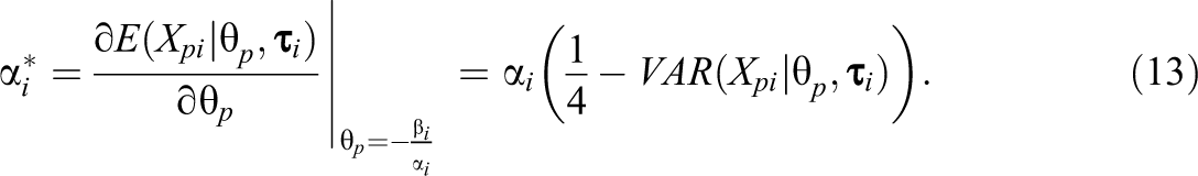
For the ${\text{α}}_i$ and ${\text{β}}_i$ parameters, the estimates from the beta-IRT and simplex-IRT model can also readily be compared as both parameters occur in the same logistic function between the conditional mean of $X_{pi}$ and ${\text{θ}}_p$ (i.e., Equations 6 and 9). However, for the S_B -IRT model, these parameters are on a different scale as the conditional mean of $X_{pi}$ is not a logistic function of ${\text{θ}}_p$ , even though the function is S-shaped. Yet, there is a transformation possible, which enables comparability of both ${\text{α}}_i$ and ${\text{β}}_i$ across models. First, as noted above, for the S_B -IRT model, it holds that $E\left(X_{pi}{\text{|θ}}_p,{\tau }_i\right)=\frac{1}{2}$ for ${\text{θ}}_p=-\frac{{\text{β}}_i}{{\text{α}}_i}$ , which is also true for the beta-IRT model and the simplex model. Therefore, by relying on ${\text{β}}_i^{*}=-\frac{{\text{β}}_i}{{\text{α}}_i}$ , the item easiness parameters can be meaningfully compared across models. To enable comparison of the discrimination parameters, we focus on ${\text{α}}_i^{*}$ , which denotes the maximum slope of $E\left(X_{pi}{\text{|θ}}_p,{\tau }_i\right)$ with respect to ${\text{θ}}_p$ . As is well known, in a logistic IRT model like Equations 6 and 9, the curve has its maximum slope at ${\text{θ}}_p=-\frac{{\text{β}}_i}{{\text{α}}_i}$ and is equal to ${\text{α}}_i^{*}=\frac{1}{4}{\text{α}}_i$ . Although the S_B -IRT model does not rely on a logistic function for $E\left(X_{pi}{\text{|θ}}_p,{\tau }_i\right)$ , it has been shown that the maximum slope in the S_B -IRT model also occurs at ${\text{θ}}_p=-\frac{{\text{β}}_i}{{\text{α}}_i}$ with the slope being given by (see, e.g., Ferrando, 2002)

${\text{α}}_i^{\text{*}}={\frac{\partial E\left(X_{pi}{\text{|θ}}_p,{\tau }_i\right)}{\partial {\text{θ}}_p}|}_{{\text{θ}}_p=-\frac{{\text{β}}_i}{{\text{α}}_i}}={\text{α}}_i\left(\frac{1}{4}-VAR\left(X_{pi}{\text{|θ}}_p,{\tau }_i\right)\right).$

13

As a result, using Equation 13, ${\text{α}}_i^{*}$ from the S_B -IRT model can meaningfully be compared to ${\text{α}}_i^{*}$ from the beta-IRT and simplex-IRT models.

As the normal-IRT model does not account for the bounded nature of the responses, it is misspecified by definition. However, the model may provide a reasonable approximation in some situations (Ferrando, 2002). To enable a meaningful comparison of the parameters, similarly as above, we define ${\text{β}}_i^{*}$ as the ${\text{θ}}_p$ value in the normal-IRT model for which $E\left(X_{pi}{\text{|θ}}_p,{\tau }_i\right)=\frac{1}{2}$ , which is ${\text{β}}_i^{*}=\frac{\frac{1}{2}-{\beta }_i}{{\text{α}}_i}$ . In addition, because in the normal-IRT model the slope of $E\left(X_{pi}{\text{|θ}}_p,{\tau }_i\right)$ with respect to ${\text{θ}}_p$ is constant, ${\text{α}}_i$ is equal to the maximum slope, that is, ${\text{α}}_i^{*}={\text{α}}_i$ . Thus, using these results, the parameters from the normal-IRT model can be compared to the transformed parameters from the bounded IRT models.

Two Motivating Examples: Consequences of Zero and One Inflation

Except for the normal-IRT models, all models above are unsuitable for responses in the closed interval [0,1]. That is, for $X_{pi}=0$ or $X_{pi}=1$ , density $f\left(X_{pi}{\text{|θ}}_p,{\tau }_i\right)$ in the beta-IRT model is either equal to 0 or equal to $\infty$ (depending on $a_{pi}$ and $b_{pi}$ in Equation 3) making the log-likelihood infinite for observations on the bounds of the response variable. In addition, for the S_B -IRT and simplex-IRT models, the densities are undefined at $X_{pi}=0$ and $X_{pi}=1$ . In practice, researchers recode responses on the bounds to prevent problems with the likelihood and to enable application of the models above. That is, 0 responses are recoded, so that they are slightly above the lower bound (e.g., to 1e-5), and 1 responses are recoded, so that they are slightly below the upper bound (e.g., to 1 – 1e-5). However, even though the likelihoods of the models are now tractable, the models cannot account for an excess of scores near the bounds. Below, we present a real data example and a simulated data example to show that the consequences of not accounting for zero and one inflation can be quite severe.

Example 1: Adjectives Checklist

We took two scales from the Adjectives Checklist (ACL; Gough, & Heilbrun, 1980) data ( $N=244)$ that are analyzed in more depth in the real data illustration section. The first scale is the Affiliation scale (10 bounded continuous items), for which both end points of the response scale are hardly used (i.e., there is hardly zero or one inflation, only four subjects used the lower end point once, the upper end point is not used at all). The second scale is the Abasement (also 10 bounded continuous items), for which the lower end point of the response scale is used more frequently resulting in zero inflation. That is, the lower end point of the scale is used in 10.75% of the responses on average across the items from the scale.

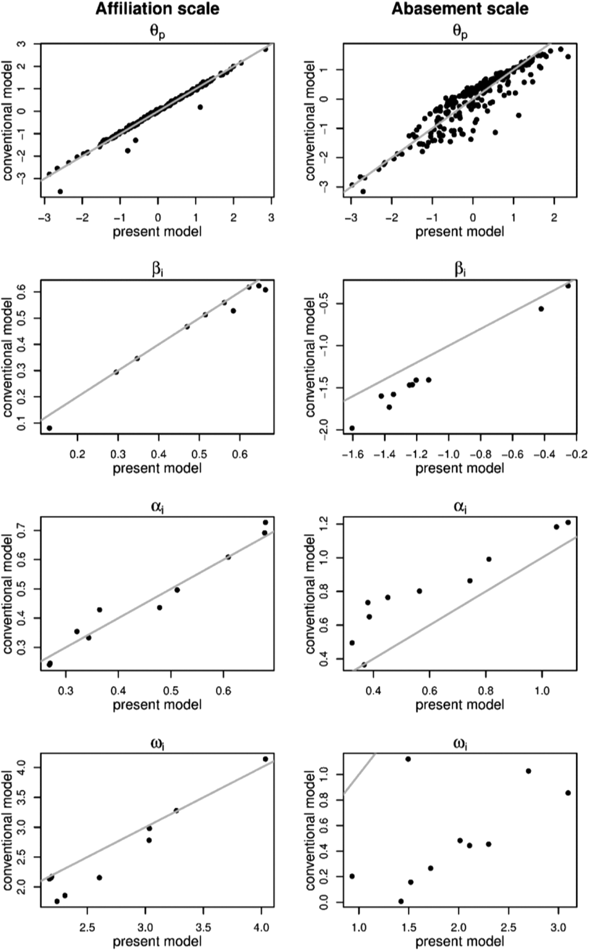
To these data, we fit the conventional beta-IRT model for open interval data from Equations 3 through 5 and the zero-one inflated extension proposed in this article. To enable application of the conventional model to the closed interval data from the ACL, we recoded 0 into 1e-5 and 1 into 1 – 1e-5 for the conventional model application. See Figure 3 for a plot of the estimates of ${\text{θ}}_p$ , ${\text{β}}_i$ , ${\text{α}}_i$ , and ${\text{ω}}_i$ in the conventional model and the estimates in the proposed model. If the estimates from the two models agree, they should scatter around the straight gray line. As can be seen, for the Affiliation scale with hardly any zero inflation, the estimates seem to agree. However, for the Abasement scale with substantial zero inflation, the estimates are systematically different for the item parameters and are very variable in the case of ${\text{θ}}_p$ as compared to the Affiliation scale without inflation.

The zero inflation in this real data example thus seems to affect the estimates from the conventional beta-IRT model. This is also true for the other models discussed above (the simplex and S_B models). However, of course, a more systematic approach is needed to demonstrate this. Therefore, below we verify this finding in a simulated data example.

Figure 3.

Plots of the parameter estimates for the conventional beta-item response theory model (y-axis) and the proposed zero and one inflated model (x-axis) for the Affiliation scale (hardly any zero and one inflation) and for the Abasement scale (on average 10.75% zero inflation across items).

Example 2: Simulated Data

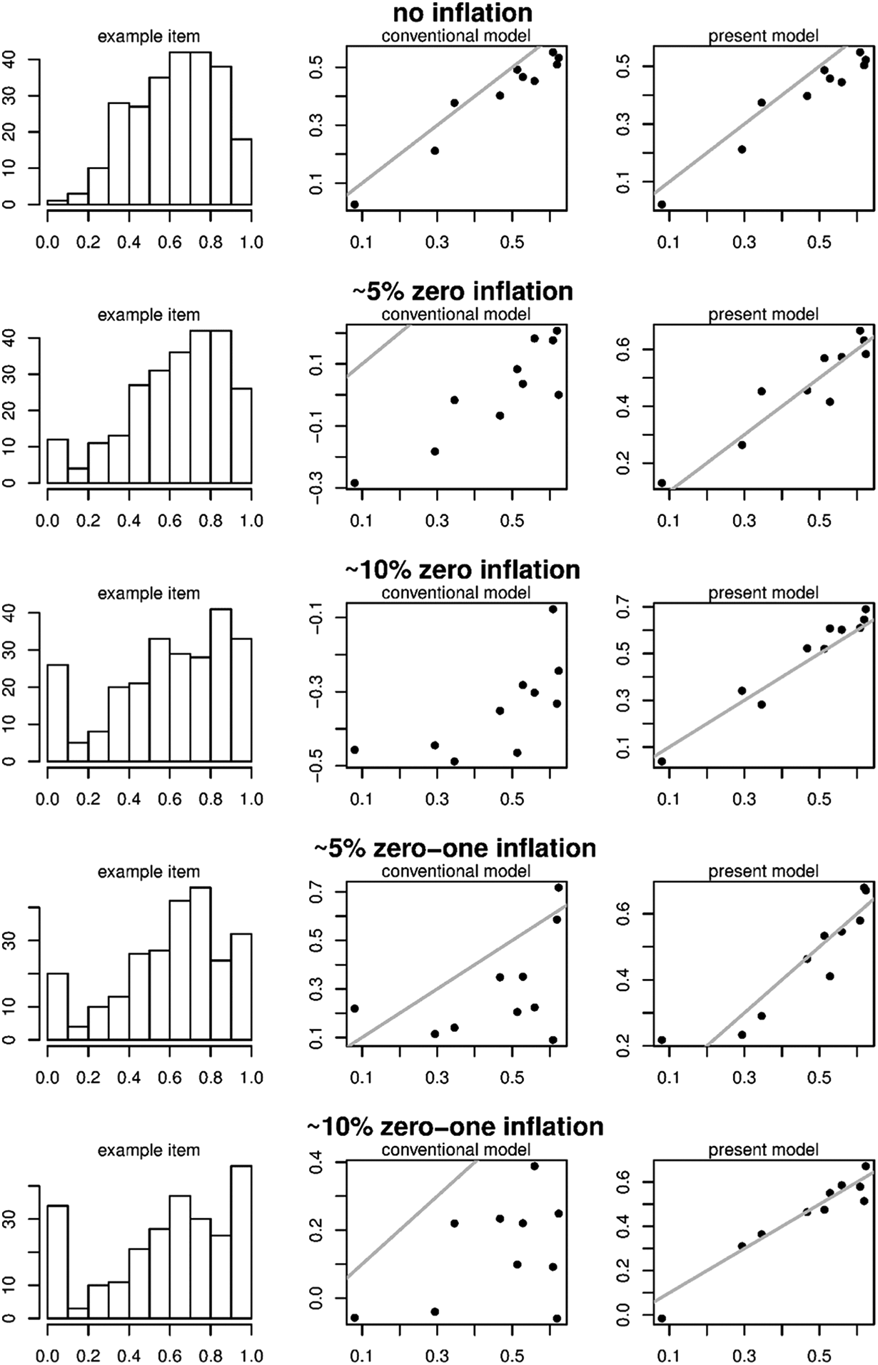
We simulated seven datasets according to the conventional beta-IRT model using $N=244$ and $n=10$ similar to the real data above. The true item parameters ${\text{α}}_i$ , ${\text{β}}_i$ , and ${\text{ω}}_i$ were set to the estimates as found for the Affiliation scale above. Person parameters ${\text{θ}}_p$ are drawn from a normal distribution. In these data, we increased the amount of zero and one inflation using the newly proposed model (which will be discussed in more detail below). Specifically, we considered the scenarios, in which 0%, approximately 5%, or approximately 10% of the scores on each item are in the lower and/or upper end point. ¹ We considered the following scenarios: (1) no inflation, (2) 5% zero inflation, (3) 10% zero inflation, (4) 5% one inflation, (5) 10% one inflation, (6) 5% zero and 5% one inflation, and (7) 10% zero and 10% one inflation. See the left column of plots in Figure 4 or 5 for the distribution of Item 1 in Scenarios 1, 2, 3, 6, and 7.

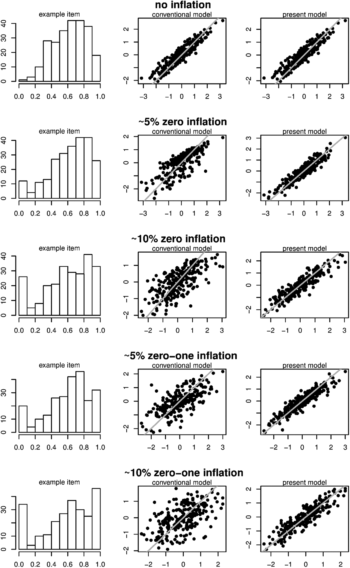
To these seven datasets, we fit the conventional beta-IRT model for open interval data from Equations 3 through 5. To enable application of this model to the closed interval data from Scenarios 2 through 7, we recoded 0 into 1e-5 and 1 into 1 – 1e-5. See Figures 4 and 5 for the estimates of, respectively, ${\text{β}}_i$ and ${\text{θ}}_p$ in the conventional model (left column of plots) and the estimates in the proposed data generating model (right column of plots) in Scenarios 1, 2, 3, 6, and 7. As can be seen, for the proposed model, the estimates of both ${\text{β}}_i$ and ${\text{θ}}_p$ seem acceptably close to the true parameter values, while for the conventional model, the estimates are biased for ${\text{β}}_i$ and have increased variability for ${\text{θ}}_p$ . Results for Scenarios 4 and 5 (which are not in the figure) are comparable to the results from Scenarios 2 and 3. In addition, the effect on the discrimination parameters ${\text{α}}_i$ is comparable to the effect on ${\text{θ}}_p$ (i.e., increased variability in the estimates). Overall, it seems thus desirable to have an IRT approach available to takes zero and one inflation into account.

Figure 4.

Left column: Histograms of an example item (Item 1) in the different scenarios. Middle column: Estimates of the conventional beta-item response theory model (x-axis) and the true values (y-axis) for ${\mathit{\text{β}}}_{\text{i}}$ in the different scenarios. Right column: Estimates of the proposed model (x-axis) and the true values (y-axis) for ${\mathit{\text{β}}}_{\text{i}}$ in the different scenarios. The gray line indicates a one-to-one correspondence.

Figure 5.

Left column: Histograms of an example item (Item 1) in the different scenarios. Middle column: Estimates of the conventional beta-item response theory model (x-axis) and the true values (y-axis) for ${\mathit{\text{θ}}}_{\text{p}}$ in the different scenarios. Right column: Estimates of the proposed model (x-axis) and the true values (x-axis) for ${\mathit{\text{θ}}}_{\text{p}}$ in the different scenarios. The gray line indicates a one-to-one correspondence.

A Zero and One Inflated Bounded IRT Approach

Here, we present the zero and one inflated approach illustrated above. The idea is that we model a dummy variable, $Z_{pi}$ , which codes three possible outcomes of the response process:

$Z_{pi}=0$ if respondent p decides to score on the lower boundary of item i.

$Z_{pi}=1$ if respondent p decides to score between the lower and upper boundary of item i.

$Z_{pi}=2$ if respondent p decides to score on the upper boundary of item i.

Next, $Z_{pi}$ is submitted to a logistic graded response model (Samejima, 1969) with category threshold parameter ${\text{γ}}_{1i}\text{'}$ and ${\text{γ}}_{2i}\text{'}$ , for which it holds that ${\text{γ}}_{2i}^{\text{'}}<{\text{γ}}_{1i}^{\text{'}}$ , so that

$P\left(Z_{pi}\ge c{\text{|θ}}_p,{\tau }_i\right)=\text{ψ}\left({\text{α}}_i{\text{θ}}_p+{\text{γ}}_{ci}^{\text{'}}\right),\text{ for }c=1,2$

14

where ${\text{α}}_i$ and ${\text{θ}}_p$ are from the model under consideration, and $P\left(Z_{pi}\ge c{\text{|θ}}_p,{\tau }_i\right)=1$ for $c=0$ . Next, to facilitate interpretation, we use ${\text{γ}}_{0i}=-{\text{γ}}_{1i}^{\text{'}}$ and ${\text{γ}}_{1i}=-{\text{γ}}_{2i}^{\text{'}}$ , so that in the final model (see below), parameter ${\text{γ}}_{0i}$ directly models the conditional probability of $X_{pi}=0$ , and parameter ${\gamma }_{1i}$ directly models the conditional probability of $X_{pi}=1$ . Note that now, ${\text{γ}}_{1i}>{\text{γ}}_{0i}$ . The probability distribution of $Z_{pi}$ is then given by

$P\left(Z_{pi}=0{\text{|θ}}_p,{\tau }_i\right)=\text{ψ}\left({\text{γ}}_{0i}-{\text{α}}_i{\text{θ}}_p\right),$

$P\left(Z_{pi}=1{\text{|θ}}_p,{\tau }_i\right)=\text{ψ}\left({\text{γ}}_{1i}-{\text{α}}_i{\theta }_p\right)-\text{ψ}\left({\text{γ}}_{0i}-{\text{α}}_i{\text{θ}}_p\right),$

$P\left(Z_{pi}=2{\text{|θ}}_p,{\tau }_i\right)=1-\text{ψ}\left({\text{γ}}_{1i}-{\text{α}}_i{\text{θ}}_p\right).$

15

The final model consists of the joint conditional density of $Z_{pi}$ and $X_{pi}$ , which will be denoted by $k(.)$ . As $Z_{pi}$ is deterministically related to $X_{pi}$ , $Z_{pi}$ itself can be neglected. Therefore, the final model is defined according to

$k\left(X_{pi}{\text{|θ}}_p,{\tau }_i\right)=\text{ψ}\left({\text{γ}}_{0i}-{\text{α}}_i{\text{θ}}_p\right)\text{ for }{X}_{pi}=0,$

$k\left(X_{pi}{\text{|θ}}_p,{\tau }_i\right)=\left\{\psi \left({\text{γ}}_{1i}-{\text{α}}_i{\text{θ}}_p\right)-\text{ψ}\left({\text{γ}}_{0i}-{\text{α}}_i{\text{θ}}_p\right)\right\}\times f\left(X_{pi}{\text{|θ}}_p,{\tau }_i\right)\text{ for }0<X_{pi}<1,$

$k\left(X_{pi}{\text{|θ}}_p,{\tau }_i\right)=1-\text{ψ}\left({\text{γ}}_{1i}-{\text{α}}_{\text{i}}{\text{θ}}_p\right)\text{ for }{X}_{pi}=1,$

16

where $f(.)$ corresponds to the density from the original models above and ${\tau }_i$ contains the item parameters of that model including ${\text{γ}}_{0i}$ and ${\text{γ}}_{1i}$ .

A mechanism similar to the above is used by Ospina and Ferrari (2010, 2012) to model zero or one inflation in the beta distribution and beta regression models. In those models however, $k\left(X_{pi}{\text{|θ}}_p,{\tau }_i\right)$ is estimated freely for $X_{pi}=0$ or for $X_{pi}=1$ (i.e., the proportion of zeros or ones in the data), while here these probabilities are constrained according to the IRT model. These constraints make sure that information about the IRT parameters ${\text{α}}_i$ , ${\text{β}}_i$ , and ${\text{θ}}_p$ is drawn from the zero and one scores. If estimated freely in the present approach, the zero and one scores will not contribute to the parameter estimation of these IRT parameters. An addition difference between the present work and the work by Ospina and Ferrari is that we consider zero and one inflation simultaneously, so that $Z_{pi}$ has three levels as discussed above. Ospina and Ferrari only considered zero or one inflation, by which $Z_{pi}$ only has two levels. Accommodating both zero and one inflation is desirable in the present IRT case as in continuous items, both end points may be used by the subjects.

Due to the inflation mechanism introduced above, the test information function of the models will change. The derivation of the test information function for the zero and one inflated bounded IRT model is given in the Appendix. Most importantly, the item and test information includes a contribution by the information from the zero and one scores and a contribution by the regular test information function $I\left({\text{θ}}_p\right)$ from the bounded IRT model $f\left(X_{pi}{\text{|θ}}_p,{\tau }_i\right)$ used for $0<X_{pi}<1$ in Equation 16. Note that for the S_B -IRT model, the resulting test information function is not constant anymore but has an inverted U-shape. The exact shapes of the test information functions are illustrated later for the different models.

Estimation and Model Comparison

Parameter Estimation

We implemented the models above in a Bayesian Markov Chain Monte Carlo (MCMC) framework. If $\theta$ denotes a vector of ${\text{θ}}_1$ ,…, ${\text{θ}}_N$ , T denotes a matrix with the stacked ${\tau }_i$ vectors for $i=1,\dots ,n$ , and X denotes the $N\times n$ matrix of item responses, then, the full posterior is proportional to

$p\left(\theta ,T\text{|}X\right)\propto s\left(\theta ,T\text{|}X\right),$

$s\left(\theta ,T\text{|}X\right)={{\displaystyle \prod }}_{p=1}^N{{\displaystyle \prod }}_{i=1}^{n}k\left(X_{pi}{\text{|θ}}_p,{\tau }_i\right)h\left({\tau }_i\right)g\left({\text{θ}}_p\right),$

17

where $k(.)$ is given above. For all models, ${\tau }_i$ contains $\text{log}\left({\text{α}}_i\right)$ , ${\text{β}}_i$ , ${\text{γ}}_{0i}$ , and ${\text{γ}}_{1i}$ . In addition, ${\tau }_i$ contains $\text{log}\left({\text{δ}}_i\right)$ for the S_B -IRT model, ${\text{ω}}_i$ for the beta-IRT model, and $\text{log}\left({\phi }_i\right)$ for the simplex-IRT model. Note that the number of free parameters is thus equal to $N\times 5n$ for all models. To facilitate parameter estimation, we estimate the untransformed parameters (i.e., ${\text{α}}_i$ and ${\text{β}}_i$ instead of ${\text{α}}_i^{*}$ and ${\text{β}}_i^{*}$ ) as this parameterization is more stable for ${\text{β}}_i$ . However, the parameters can always be transformed afterwards. In addition, we estimate $\text{log}\left({\text{α}}_i\right)$ to avoid sign switching during estimation. In all models, the prior distribution of ${\text{θ}}_p$ , $g()$ , is specified to be a Normal(0,1) distribution, and the prior distribution of ${\tau }_i$ is specified to be independent Normal(0,10) distributions for each element of ${\tau }_i$ . For ${\text{γ}}_{1i}$ , the normal prior is truncated below ${\text{γ}}_{0i}$ to ensure that ${\text{γ}}_{1i}>{\text{γ}}_{0i}$ . The models are implemented in Stan using Rstan (Stan Development Team, 2019) in the R statistical computing environment (R core team, 2019). The scripts to fit the different models are available from www.dylanmolenaar.nl.

Model Comparison Using the Log Marginal Likelihood

To be able to select between the different models, we propose to use the fully marginalized log-likelihood, that is:

$\ell \left(X\right)=\text{ln}ℒ\left(X\right)={\displaystyle \sum }_{p=1}^N\text{ln}\underset{\text{θ}}{\overset{ }{{\displaystyle \int }}}\left({\displaystyle \prod }_{i=1}^n\underset{\tau }{\overset{ }{{\displaystyle \int }}}k\left(X_{pi}{\text{|θ}}_p,{\tau }_i\right)h\left({\tau }_i\right)d\tau \right)g\left({\text{θ}}_p\right)d\text{θ .}$

18

The advantage of the log marginal likelihood is that it incorporates a penalty for model complexity in a natural way. As determining model complexity of the models under investigation in this study is not straightforward, we consider the log marginal likelihood better suitable to select between competing models as compared to, for example, the Deviance Information Criterion (DIC), Watanabe-Akaike Information Criterion (WAIC), and Bayesian Information Criterion (BIC). The marginal likelihood is the key ingredient of Bayes’s factors commonly used for selection between two competing models. Here, we use the log marginal likelihood as a fit index on its own by selecting the model with the highest log marginal likelihood as best fitting model; however, calculation of Bayes’s factors is straightforward, which is illustrated in the real data application. Calculating the fully marginalized log-likelihood directly is infeasible due to the high number of nested integrals. However, the marginal likelihood can be approximated using bridge sampling (e.g., Gronau et al., 2017; Meng & Wong, 1996).

Simulation Study A: Item Parameter Recovery and Model Fit

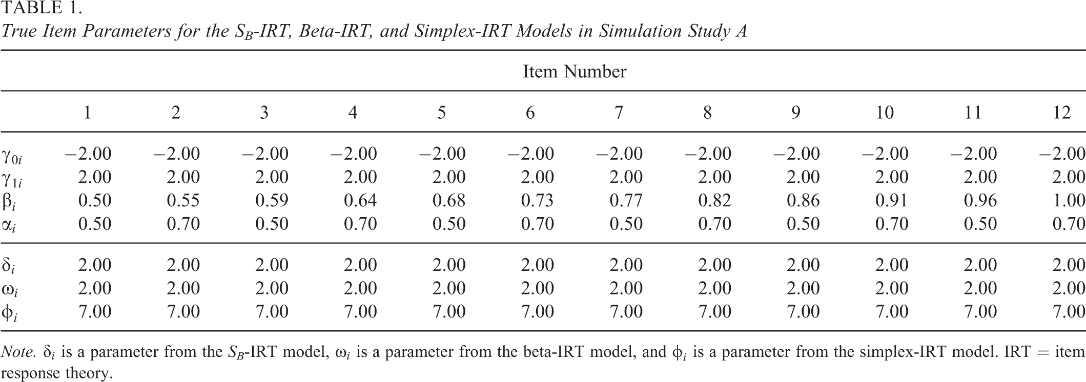
In this simulation study, we simulate data according to the zero and one inflation mechanism in Equation 16 with $f(X_{pi}|{\text{θ}}_p,{\tau }_i)$ given by either the S_B -IRT model (Equation 1), the beta-IRT model (Equations 3 –5) or the simplex-IRT model (Equation 7). We use the same item parameters across replications to study parameter recovery of the item parameters. We use 12 items with true values given in Table 1. The true values for ${\text{γ}}_{0i}$ and ${\text{γ}}_{1i}$ correspond to the ∼10% zero and one inflation scenario from Figures 4 and 5, which we chose because it is the most challenging scenario for the inflated IRT model due to the reasonably large inflation in the data. In addition, for ${\text{α}}_i$ and ${\text{β}}_i$ , we use the same values across the different models as these parameters are either comparable (between the beta-IRT model and the simplex-IRT model due to Equations 6 and 9) or highly related (between the S_B -IRT model and the other models). For the dispersion parameters, we use different values for the models as these parameters have different scales across the models. To give an illustration of how the simulated data look, we plotted the resulting densities and information functions for the different models in Figure 6 for Item 5. The distributions differ across items but are generally left-skewed comparable to Figure 6.

Table 1.

True Item Parameters for the S_B-IRT, Beta-IRT, and Simplex-IRT Models in Simulation Study A

	Item Number
	1	2	3	4	5	6	7	8	9	10	11	12
${\text{γ}}_{0i}$	−2.00	−2.00	−2.00	−2.00	−2.00	−2.00	−2.00	−2.00	−2.00	−2.00	−2.00	−2.00
${\text{γ}}_{1i}$	2.00	2.00	2.00	2.00	2.00	2.00	2.00	2.00	2.00	2.00	2.00	2.00
${\text{β}}_i$	0.50	0.55	0.59	0.64	0.68	0.73	0.77	0.82	0.86	0.91	0.96	1.00
${\text{α}}_i$	0.50	0.70	0.50	0.70	0.50	0.70	0.50	0.70	0.50	0.70	0.50	0.70
${\text{δ}}_i$	2.00	2.00	2.00	2.00	2.00	2.00	2.00	2.00	2.00	2.00	2.00	2.00
${\text{ω}}_i$	2.00	2.00	2.00	2.00	2.00	2.00	2.00	2.00	2.00	2.00	2.00	2.00
${\phi }_i$	7.00	7.00	7.00	7.00	7.00	7.00	7.00	7.00	7.00	7.00	7.00	7.00

Note. ${\text{δ}}_i$ is a parameter from the S_B -IRT model, ${\text{ω}}_i$ is a parameter from the beta-IRT model, and ${\phi }_i$ is a parameter from the simplex-IRT model. IRT = item response theory.

Figure 6.

Density and item information function of Item 5 ( ${\mathit{\text{β}}}_{\text{i}}=0.685,{\mathit{\text{α}}}_{\text{i}}=0.5,{\mathit{\text{γ}}}_0=-2,{\mathit{\text{and γ}}}_1=2)$ for the S_B-IRT model ( ${\mathit{\text{δ}}}_{\text{i}}=2$ ), the beta-IRT model ( ${\text{ω}}_{\text{i}}=2$ ), and the simplex-IRT model ( ${\varphi }_i=7)$ . The zero and one inflation is not incorporated in the density plots as these are reflected by probabilities and not by densities. The zero and one inflation is however incorporated in the item information function. IRT = item response theory.

The true item parameter values in this study are inspired by the real dataset used in the example below. That is why the values of the item easiness parameters ${\text{β}}_i$ are chosen to represent a relatively easy test (this is what was found throughout most of the 22 scales in our real dataset, with the exception that for some scales the items are relatively difficult, but this generally only affects ${\text{β}}_i$ , so that the observed distributions are right skewed, but the simulation results below are equally applicable to these cases). We think that a relatively easy test as used in this simulation study is typical for tests with continuous items, which are mostly concerned with measuring constructs like personality and mood. Using a relatively easy test for the simulation does however result in smaller information about ${\text{θ}}_p$ in its upper range. As the test information functions of the models differ in their shape, the relative easiness of the test will affect parameter estimates differently across the models. We think that this is interesting, as this will also happen in practice. However, this differential effect of the distribution of item easiness should be kept in mind when interpreting the results.

In this study, we use sample sizes of 50, 100, and 200 persons. In addition, we use 100 replications. In each replication, we sample ${\text{θ}}_p$ from a Normal(0,1) distribution. To the data in each replication, we fit the three bounded-IRT models subject to zero and one inflation (Equation 16). In addition, we estimate the unbounded normal-IRT model to investigate the effect of neglecting the bounded nature of the data. To enable a fair comparison to the other models, this model is also subjected to the zero and one inflation in Equation 16. Finally, the models are compared using the log marginal likelihood discussed above. We also considered the DIC (Spiegelhalter et al., 2002) and WAIC (Watanabe, 2010) model fit indices, to have a reference to compare the performance of the log marginal likelihood to. However, note that there are other fit indices that may perform better than the DIC and WAIC (e.g., the LOO-IC; Vehtari et al., 2017).

Results

Parameter Recovery of the True Model

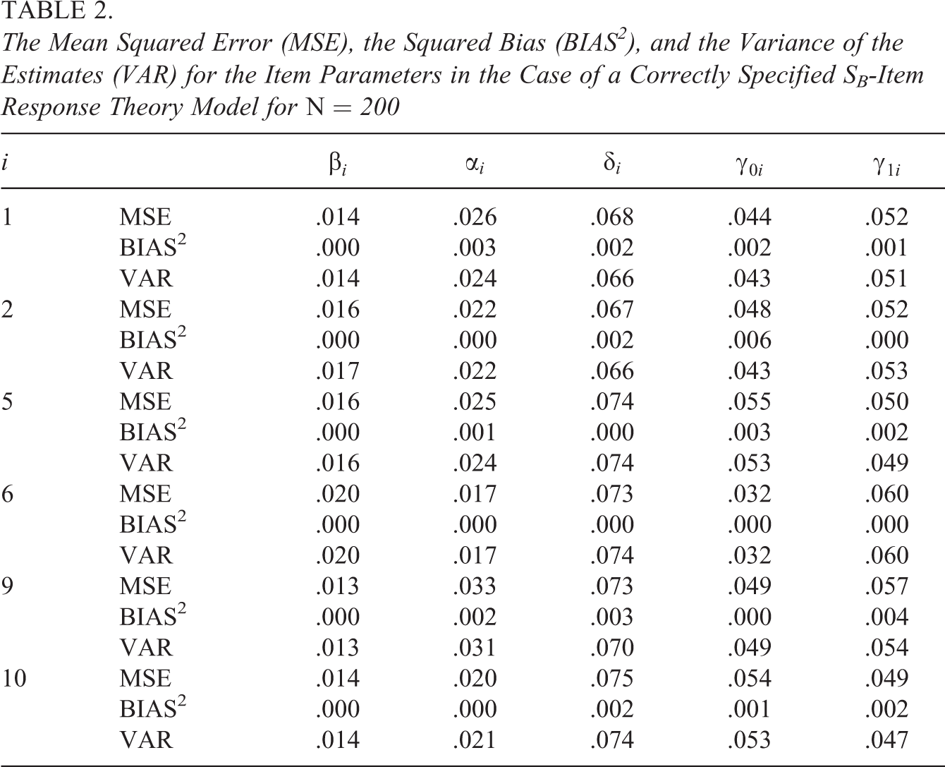
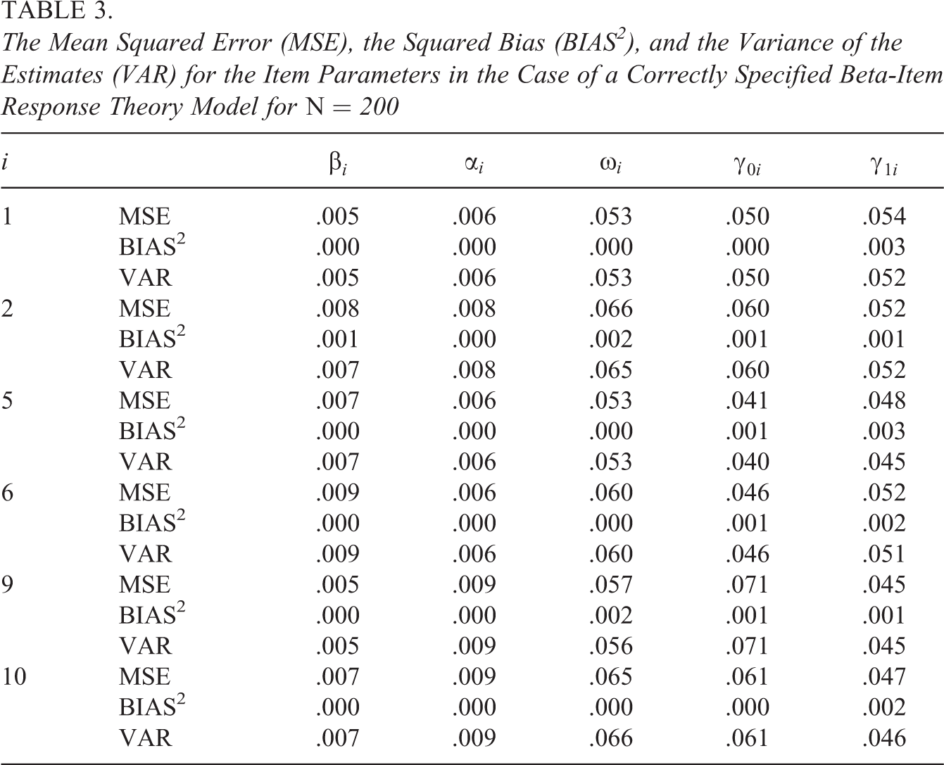
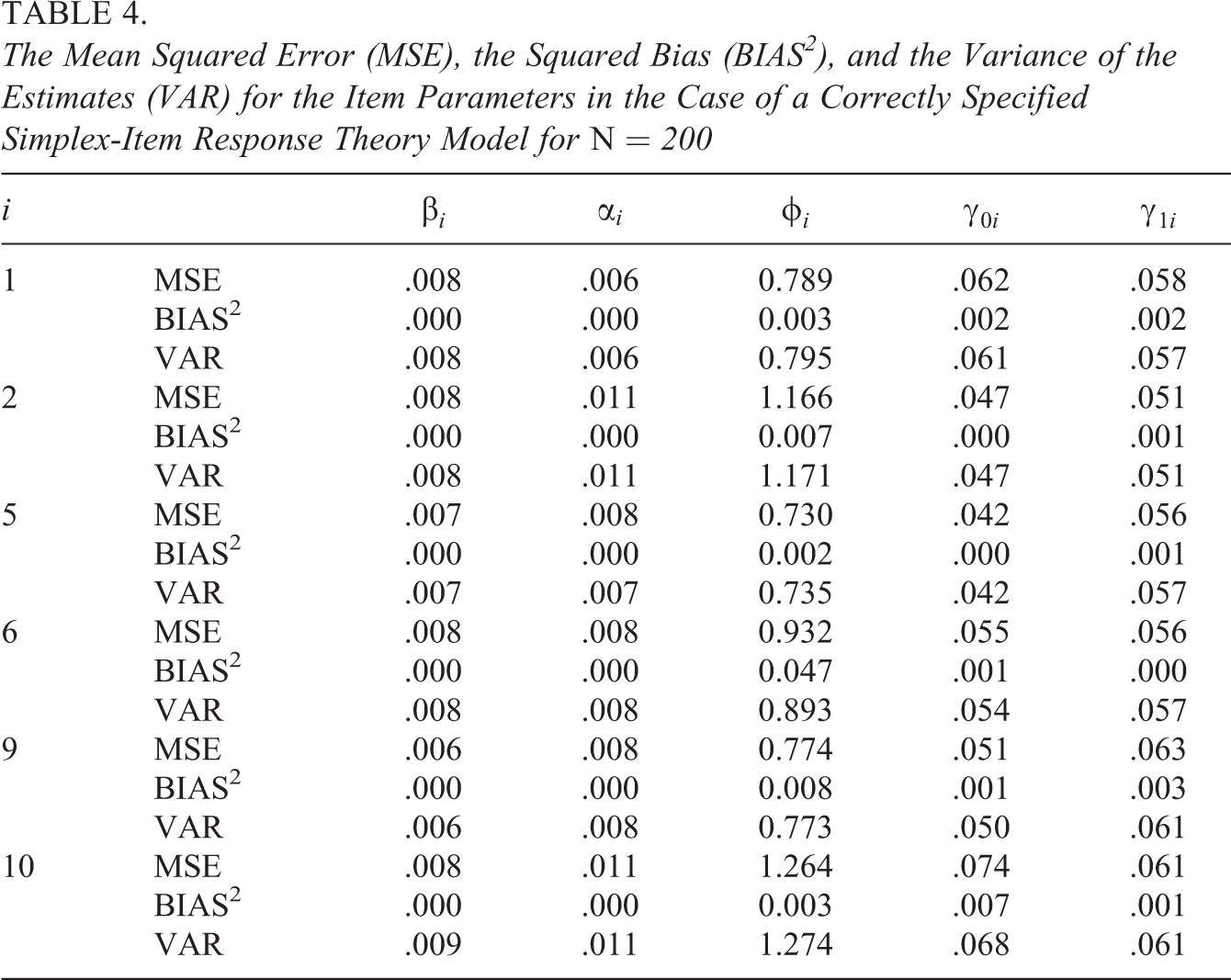
To study the parameter recovery, we focus on the posterior mean estimates of the correctly specified models in the different conditions in the simulation study for $N=200$ . Tables 2 through 4 depict the mean squared error (MSE), the squared bias (BIAS²), and the variance of the estimates (VAR) for the parameters of respectively the S_B -IRT, the beta-IRT, and the simplex-IRT models for Items 1, 2, 5,6, 9, and 10 in the $N=200$ condition. To save space, we selected this subset to represent a mix of odd and even items (which differ in their item discrimination, see Table 1). For an adequate parameter recovery, the MSE is approximately equal to the VAR, which results in a BIAS² close to 0. As can be seen, for all parameters in all models, the parameter recovery seems acceptable with the difference between MSE and VAR being only notable in the third decimal. The results for the other sample size conditions ( $N=50$ and $N=100$ ) are acceptable with adequate parameter recovery and a minor bias in the case of $N=50$ , where the estimates are pulled toward their prior means.

Table 2.

The Mean Squared Error (MSE), the Squared Bias (BIAS²), and the Variance of the Estimates (VAR) for the Item Parameters in the Case of a Correctly Specified S_B-Item Response Theory Model for $\text{N}=\mathit{\text{200}}$

i		${\text{β}}_i$	${\text{α}}_i$	${\text{δ}}_i$	${\text{γ}}_{0i}$	${\text{γ}}_{1i}$
1	MSE	.014	.026	.068	.044	.052
	BIAS2	.000	.003	.002	.002	.001
	VAR	.014	.024	.066	.043	.051
2	MSE	.016	.022	.067	.048	.052
	BIAS2	.000	.000	.002	.006	.000
	VAR	.017	.022	.066	.043	.053
5	MSE	.016	.025	.074	.055	.050
	BIAS2	.000	.001	.000	.003	.002
	VAR	.016	.024	.074	.053	.049
6	MSE	.020	.017	.073	.032	.060
	BIAS2	.000	.000	.000	.000	.000
	VAR	.020	.017	.074	.032	.060
9	MSE	.013	.033	.073	.049	.057
	BIAS2	.000	.002	.003	.000	.004
	VAR	.013	.031	.070	.049	.054
10	MSE	.014	.020	.075	.054	.049
	BIAS2	.000	.000	.002	.001	.002
	VAR	.014	.021	.074	.053	.047

Table 3.

The Mean Squared Error (MSE), the Squared Bias (BIAS²), and the Variance of the Estimates (VAR) for the Item Parameters in the Case of a Correctly Specified Beta-Item Response Theory Model for $\text{N}=\mathit{\text{200}}$

i		${\text{β}}_i$	${\text{α}}_i$	${\text{ω}}_i$	${\text{γ}}_{0i}$	${\text{γ}}_{1i}$
1	MSE	.005	.006	.053	.050	.054
	BIAS2	.000	.000	.000	.000	.003
	VAR	.005	.006	.053	.050	.052
2	MSE	.008	.008	.066	.060	.052
	BIAS2	.001	.000	.002	.001	.001
	VAR	.007	.008	.065	.060	.052
5	MSE	.007	.006	.053	.041	.048
	BIAS2	.000	.000	.000	.001	.003
	VAR	.007	.006	.053	.040	.045
6	MSE	.009	.006	.060	.046	.052
	BIAS2	.000	.000	.000	.001	.002
	VAR	.009	.006	.060	.046	.051
9	MSE	.005	.009	.057	.071	.045
	BIAS2	.000	.000	.002	.001	.001
	VAR	.005	.009	.056	.071	.045
10	MSE	.007	.009	.065	.061	.047
	BIAS2	.000	.000	.000	.000	.002
	VAR	.007	.009	.066	.061	.046

Table 4.

The Mean Squared Error (MSE), the Squared Bias (BIAS²), and the Variance of the Estimates (VAR) for the Item Parameters in the Case of a Correctly Specified Simplex-Item Response Theory Model for $\text{N}=\mathit{\text{200}}$

i		${\text{β}}_i$	${\text{α}}_i$	${\phi }_i$	${\text{γ}}_{0i}$	${\text{γ}}_{1i}$
1	MSE	.008	.006	0.789	.062	.058
	BIAS2	.000	.000	0.003	.002	.002
	VAR	.008	.006	0.795	.061	.057
2	MSE	.008	.011	1.166	.047	.051
	BIAS2	.000	.000	0.007	.000	.001
	VAR	.008	.011	1.171	.047	.051
5	MSE	.007	.008	0.730	.042	.056
	BIAS2	.000	.000	0.002	.000	.001
	VAR	.007	.007	0.735	.042	.057
6	MSE	.008	.008	0.932	.055	.056
	BIAS2	.000	.000	0.047	.001	.000
	VAR	.008	.008	0.893	.054	.057
9	MSE	.006	.008	0.774	.051	.063
	BIAS2	.000	.000	0.008	.001	.003
	VAR	.006	.008	0.773	.050	.061
10	MSE	.008	.011	1.264	.074	.061
	BIAS2	.000	.000	0.003	.007	.001
	VAR	.009	.011	1.274	.068	.061

Consequence of Misfit

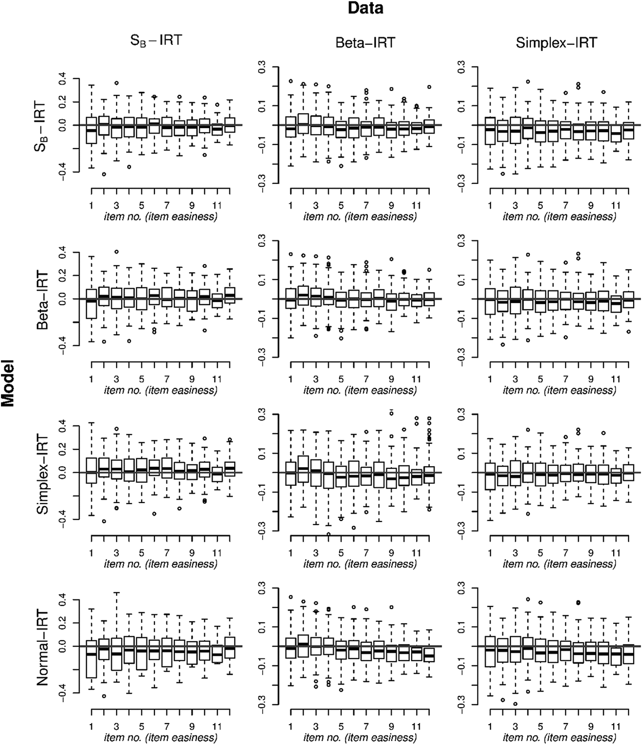
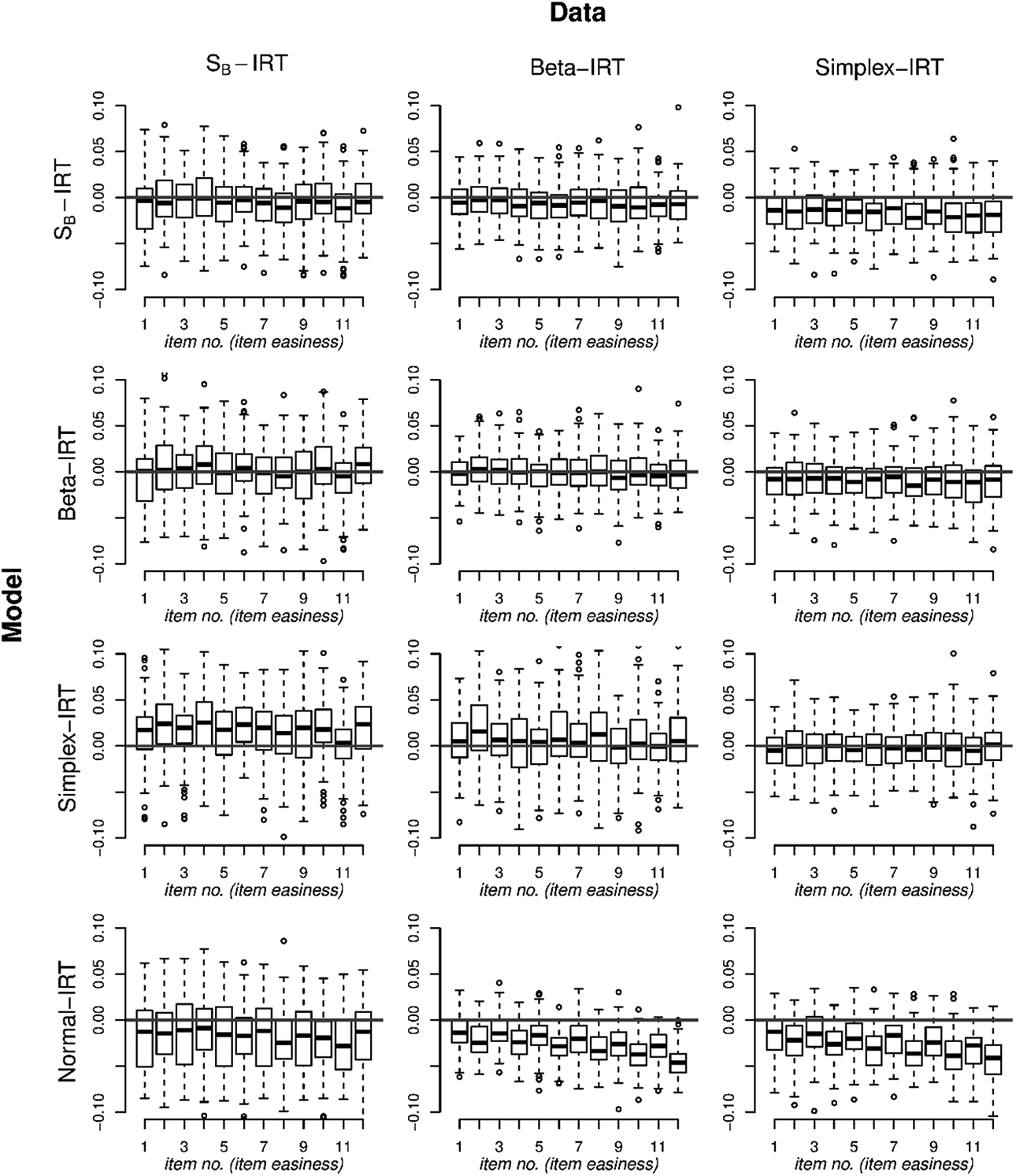
To study the consequences for the item parameters of fitting an incorrect model to the data, we focus on the parameter estimates of the discrimination parameters and the easiness parameters across the different models for the different data scenarios in the simulation study. To enable a meaningful comparison, we focus on ${\text{α}}_i^{*}$ and ${\text{β}}_i^{*}$ as discussed above. Figures 7 and 8 depict the boxplots of the errors of, respectively, $\text{exp}\left({\text{β}}_i^{*}\right)$ and ${\text{α}}_i^{*}$ across replications for the different fitted models under the different data generating scenarios for $N=200$ . We rely on $\text{exp}\left({\text{β}}_i^{*}\right)$ for clarity of the figure as in a few cases ${\text{β}}_i^{*}$ is large and negative which distorts the figure. ² From Figure 7, it can be seen that for the bounded IRT models, ${\text{β}}_i^{*}$ is hardly affected by misspecification. The only case where ${\text{β}}_i^{*}$ is slightly underestimated is in the S_B -IRT model in the case of simplex-IRT data. In the normal-IRT model, ${\text{β}}_i^{*}$ is underestimated, in all data scenarios but the bias is minor. From Figure 8, it can be seen that model misspecification has a larger effect on ${\text{α}}_i^{*}$ . That is, for the S_B -IRT model, the simplex-IRT parameters are underestimated, and for the simplex-IRT model, the S_B -IRT model parameter and the beta-IRT model parameters are overestimated. In addition, for the beta-IRT model, the simplex-IRT model parameters are underestimated. The beta-IRT model and the S_B -IRT model are less biased with respect to each other. For the normal-IRT model, ${\text{α}}_i^{*}$ is underestimated in all data scenarios with the bias being larger for the items with a larger item easiness.

Figure 7.

Boxplots of the errors in $\mathit{\text{exp}}\left({\mathit{\text{β}}}_{\text{i}}^{*}\right)$ in each bounded item response theory model (rows) for the different data generating models (columns) in Simulation Study A. The x-axis contains the individual items ( $\text{i}=\mathit{\text{1}},\mathit{\text{.12}}$ ), which are ordered on their true item easiness parameters by the design of the study.

Figure 8.

Boxplots of the errors in ${\mathit{\text{α}}}_{\text{i}}^{*}$ in each bounded item response theory model (rows) for the different data generating models (columns) in the Simulation Study A. The x-axis contains the individual items (1–12), which are ordered on their easiness.

Model Fit

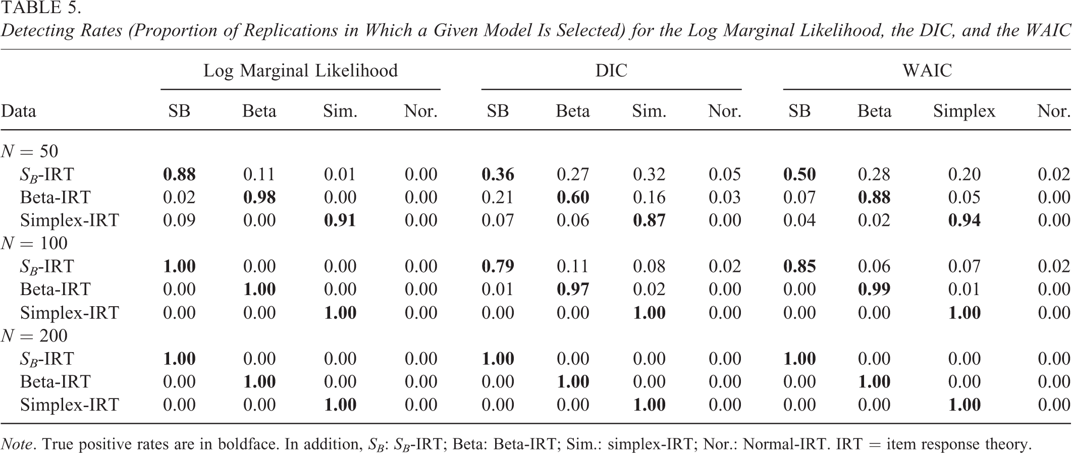
In Table 5, the proportion of replications in which a given model is selected according to the log marginal likelihood, the DIC, and the WAIC is depicted (detection rates). As can be seen, the models are well separable: For $N=50$ , the log marginal likelihood performs overall better compared to the DIC and WAIC with a true positive rate of at least 0.88. The true positive rates for the DIC are unacceptable for the S_B -IRT and the beta-IRT model (0.36 and 0.60, respectively) but acceptable although lower as compared to the log marginal likelihood- for the simplex-IRT model. The WAIC results are unacceptable for the S_B -IRT model with a true positive rate of 0.50 but acceptable for the beta-IRT model and the simplex-IRT model. For the simplex-IRT, the WAIC slightly outperforms the true positive rate of the log marginal likelihood (although the difference is insignificant, $p=.591$ ). For $N=100$ , the log marginal likelihood overall still performs best, but with smaller differences. For $N=200$ , the three fit measures perform optimal with all false positive rates equal to 0.00.

Table 5.

Detecting Rates (Proportion of Replications in Which a Given Model Is Selected) for the Log Marginal Likelihood, the DIC, and the WAIC

	Log Marginal Likelihood				DIC				WAIC
Data	SB	Beta	Sim.	Nor.	SB	Beta	Sim.	Nor.	SB	Beta	Simplex	Nor.
N = 50
SB -IRT	0.88	0.11	0.01	0.00	0.36	0.27	0.32	0.05	0.50	0.28	0.20	0.02
Beta-IRT	0.02	0.98	0.00	0.00	0.21	0.60	0.16	0.03	0.07	0.88	0.05	0.00
Simplex-IRT	0.09	0.00	0.91	0.00	0.07	0.06	0.87	0.00	0.04	0.02	0.94	0.00
N = 100
SB -IRT	1.00	0.00	0.00	0.00	0.79	0.11	0.08	0.02	0.85	0.06	0.07	0.02
Beta-IRT	0.00	1.00	0.00	0.00	0.01	0.97	0.02	0.00	0.00	0.99	0.01	0.00
Simplex-IRT	0.00	0.00	1.00	0.00	0.00	0.00	1.00	0.00	0.00	0.00	1.00	0.00
N = 200
SB -IRT	1.00	0.00	0.00	0.00	1.00	0.00	0.00	0.00	1.00	0.00	0.00	0.00
Beta-IRT	0.00	1.00	0.00	0.00	0.00	1.00	0.00	0.00	0.00	1.00	0.00	0.00
Simplex-IRT	0.00	0.00	1.00	0.00	0.00	0.00	1.00	0.00	0.00	0.00	1.00	0.00

Note. True positive rates are in boldface. In addition, S_B : S_B -IRT; Beta: Beta-IRT; Sim.: simplex-IRT; Nor.: Normal-IRT. IRT = item response theory.

Conclusion

From the above, we can conclude that the parameter recovery of the different models is acceptable with MSE’s close to the parameter variability. With respect to model selection, it appeared that for smaller sample sizes, the log marginal likelihood outperforms the DIC and WAIC, but for larger sample sizes, this difference diminishes. In addition, the three bounded IRT models are relatively robust with respect to each other in the estimation of the item easiness. However, with respect to the item discrimination, the beta-IRT and S_B -IRT models are relatively robust to each other while they are biased if the data are generated from the simplex-IRT model. In addition, the simplex-IRT model appeared to be biased with respect to the beta-IRT and S_B -IRT models. The normal-IRT model was biased in all scenarios with small effects on the easiness but relatively large effects on the discrimination parameter.

Simulation Study B: Person Parameter Recovery

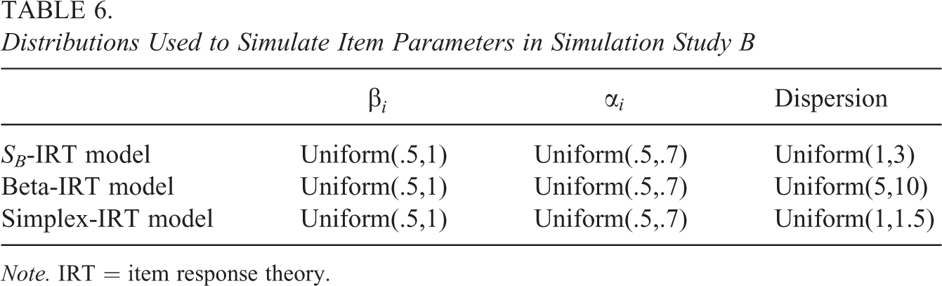
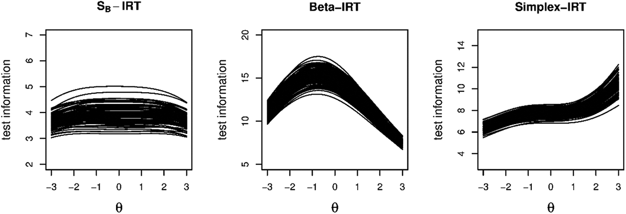
Similarly, as in Simulation Study A, we simulate data according to the zero and one inflated bounded-IRT models above. However, we now use the same values for ${\text{θ}}_p$ across replications to study parameter recovery of the person parameters. Specifically, we use the following levels for ${\text{θ}}_p$ : −3, −2.5, −2, −1.5, −1, −0.5, 0, .5, 1, 1.5, 2, 2.5, and 3. The frequency with which the different levels for ${\text{θ}}_p$ occur follows a standard normal distribution. In addition, we use 240 subjects, 6, 12, and 18 items, and 100 replications. In each replication, we sample the item parameters from a specific distribution (see Table 6). The choice for these distributions is again inspired by the real data application below. The test information across the replications on the basis of the true item parameters is depicted in Figure 9 for each model and $n=18$ . To the data in each replication, we fit the same four models as in Simulation Study A and study parameter recovery of ${\text{θ}}_p$ .

Table 6.

Distributions Used to Simulate Item Parameters in Simulation Study B

	${\text{β}}_i$	${\text{α}}_i$	Dispersion
SB -IRT model	Uniform(.5,1)	Uniform(.5,.7)	Uniform(1,3)
Beta-IRT model	Uniform(.5,1)	Uniform(.5,.7)	Uniform(5,10)
Simplex-IRT model	Uniform(.5,1)	Uniform(.5,.7)	Uniform(1,1.5)

Note. IRT = item response theory.

Figure 9.

Test information functions across replications in Simulation Study B for the different models and n = 18.

Results

For all models, a small shrinkage effect is found for the ${\text{θ}}_p$ estimates in all models and conditions. That is, due to the finite numbers of item (18 at most), the ${\text{θ}}_p$ estimates are pulled slightly to their prior mean. To be able to study parameter recovery, we adjust for the shrinkage effect by dividing the ${\text{θ}}_p$ estimates by the standard deviation of the estimates. As a result, all departures from the true ${\text{θ}}_p$ values are due to bias and not due to shrinkage.

Parameter Recovery of the True Model

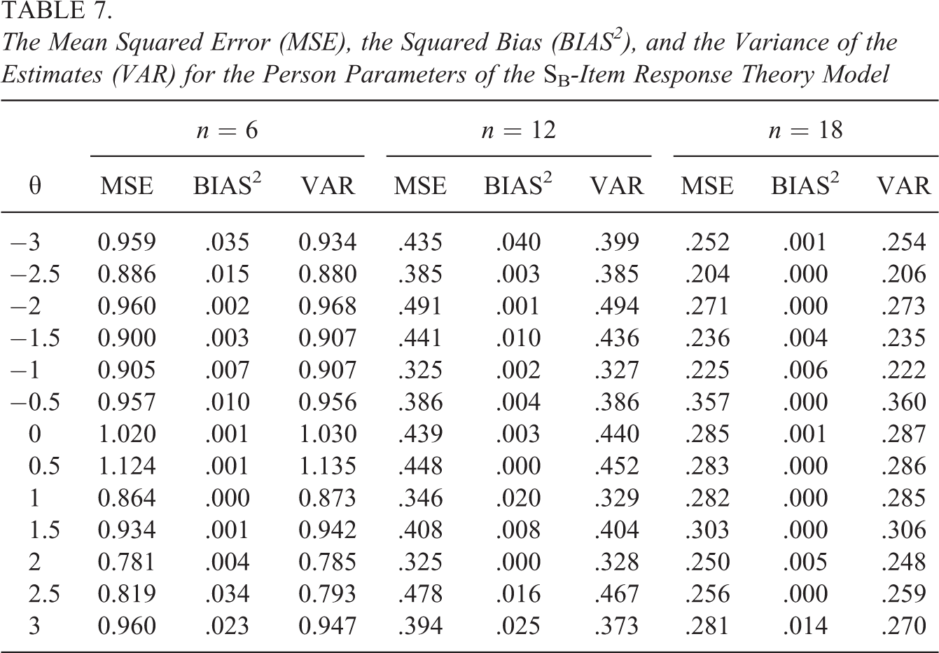
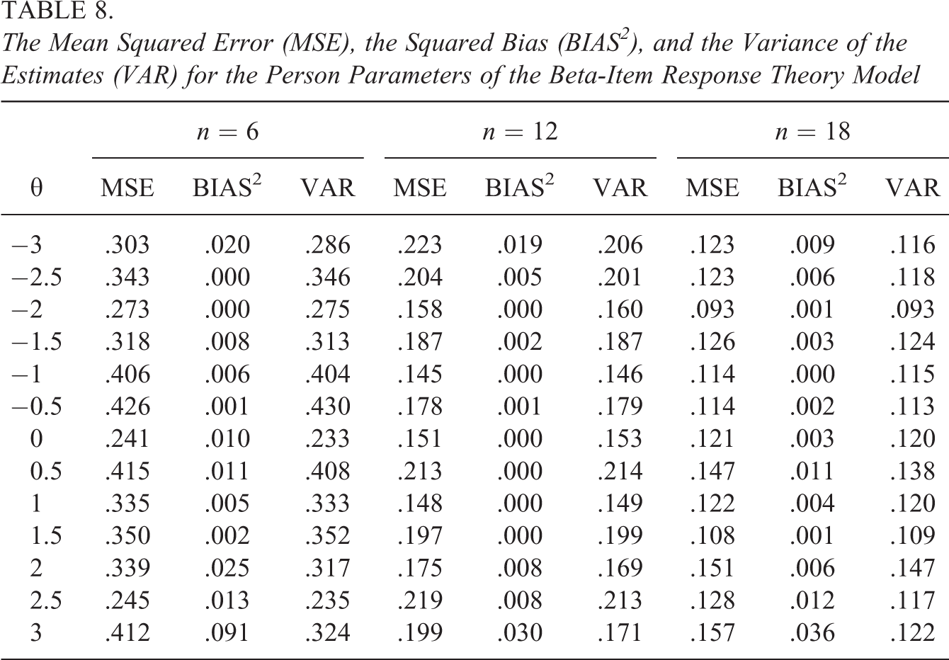
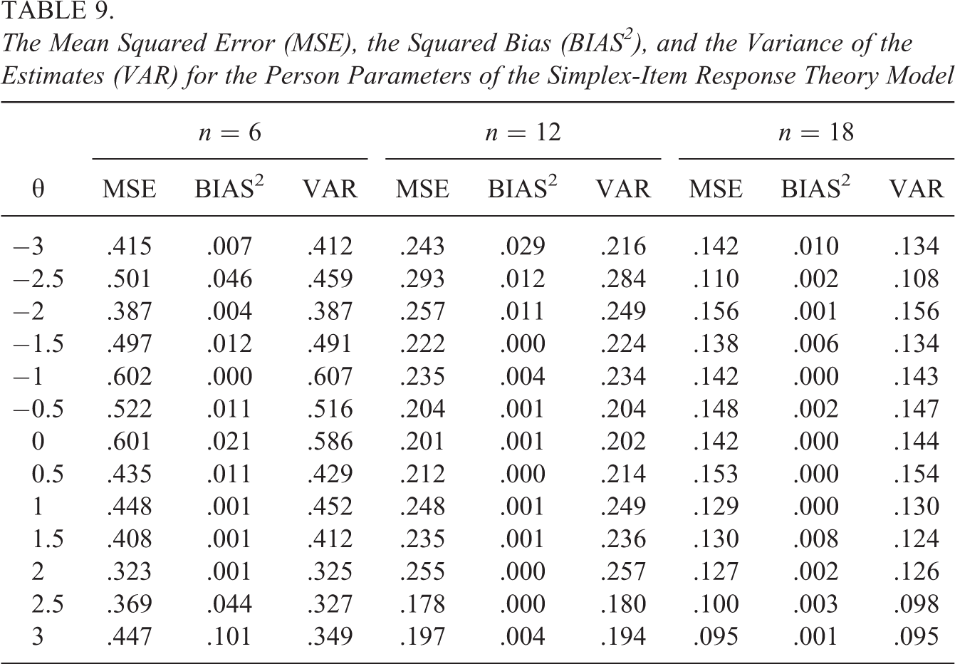
To study the parameter recovery, we focus on the estimates of the true model in the different conditions in the simulation study to see whether the expected squared bias approaches 0. Tables 7 –9 contain the MSE, BIAS², and VAR for the parameters of, respectively, the S_B -IRT, the beta-IRT, and the simplex-IRT models for the different values of ${\text{θ}}_p$ and for a different number of items. As can be seen, for all models, the parameter recovery seems acceptable with the MSE being mostly due to parameter variability and with a small to neglectable contribution of the squared bias. For six items ( $n=6)$ , bias seems slightly larger for larger absolute values of ${\text{θ}}_p$ , but this bias decreases for larger number of items. The MSE seems to follow the test information functions in Figure 9, at least for the beta-IRT and the simplex-IRT model, with the MSEs being somewhat smaller toward the upper ${\text{θ}}_p$ values for the simplex-IRT model, while being somewhat smaller in the middle ${\text{θ}}_p$ region for the beta-IRT model. Note that the values of the MSE itself cannot be compared between the models as these results are based on different data with different characteristics. For instance, the test information is overall much smaller for the data generated with the S_B model (see Figure 9), which results in overall larger MSEs.

Table 7.

The Mean Squared Error (MSE), the Squared Bias (BIAS²), and the Variance of the Estimates (VAR) for the Person Parameters of the S_B -Item Response Theory Model

	n = 6			n = 12			n = 18
$\text{θ}$	MSE	BIAS2	VAR	MSE	BIAS2	VAR	MSE	BIAS2	VAR
−3	0.959	.035	0.934	.435	.040	.399	.252	.001	.254
−2.5	0.886	.015	0.880	.385	.003	.385	.204	.000	.206
−2	0.960	.002	0.968	.491	.001	.494	.271	.000	.273
−1.5	0.900	.003	0.907	.441	.010	.436	.236	.004	.235
−1	0.905	.007	0.907	.325	.002	.327	.225	.006	.222
−0.5	0.957	.010	0.956	.386	.004	.386	.357	.000	.360
0	1.020	.001	1.030	.439	.003	.440	.285	.001	.287
0.5	1.124	.001	1.135	.448	.000	.452	.283	.000	.286
1	0.864	.000	0.873	.346	.020	.329	.282	.000	.285
1.5	0.934	.001	0.942	.408	.008	.404	.303	.000	.306
2	0.781	.004	0.785	.325	.000	.328	.250	.005	.248
2.5	0.819	.034	0.793	.478	.016	.467	.256	.000	.259
3	0.960	.023	0.947	.394	.025	.373	.281	.014	.270

Table 8.

The Mean Squared Error (MSE), the Squared Bias (BIAS²), and the Variance of the Estimates (VAR) for the Person Parameters of the Beta-Item Response Theory Model

	n = 6			n = 12			n = 18
$\text{θ}$	MSE	BIAS2	VAR	MSE	BIAS2	VAR	MSE	BIAS2	VAR
−3	.303	.020	.286	.223	.019	.206	.123	.009	.116
−2.5	.343	.000	.346	.204	.005	.201	.123	.006	.118
−2	.273	.000	.275	.158	.000	.160	.093	.001	.093
−1.5	.318	.008	.313	.187	.002	.187	.126	.003	.124
−1	.406	.006	.404	.145	.000	.146	.114	.000	.115
−0.5	.426	.001	.430	.178	.001	.179	.114	.002	.113
0	.241	.010	.233	.151	.000	.153	.121	.003	.120
0.5	.415	.011	.408	.213	.000	.214	.147	.011	.138
1	.335	.005	.333	.148	.000	.149	.122	.004	.120
1.5	.350	.002	.352	.197	.000	.199	.108	.001	.109
2	.339	.025	.317	.175	.008	.169	.151	.006	.147
2.5	.245	.013	.235	.219	.008	.213	.128	.012	.117
3	.412	.091	.324	.199	.030	.171	.157	.036	.122

Table 9.

The Mean Squared Error (MSE), the Squared Bias (BIAS²), and the Variance of the Estimates (VAR) for the Person Parameters of the Simplex-Item Response Theory Model

	n = 6			n = 12			n = 18
$\text{θ}$	MSE	BIAS2	VAR	MSE	BIAS2	VAR	MSE	BIAS2	VAR
−3	.415	.007	.412	.243	.029	.216	.142	.010	.134
−2.5	.501	.046	.459	.293	.012	.284	.110	.002	.108
−2	.387	.004	.387	.257	.011	.249	.156	.001	.156
−1.5	.497	.012	.491	.222	.000	.224	.138	.006	.134
−1	.602	.000	.607	.235	.004	.234	.142	.000	.143
−0.5	.522	.011	.516	.204	.001	.204	.148	.002	.147
0	.601	.021	.586	.201	.001	.202	.142	.000	.144
0.5	.435	.011	.429	.212	.000	.214	.153	.000	.154
1	.448	.001	.452	.248	.001	.249	.129	.000	.130
1.5	.408	.001	.412	.235	.001	.236	.130	.008	.124
2	.323	.001	.325	.255	.000	.257	.127	.002	.126
2.5	.369	.044	.327	.178	.000	.180	.100	.003	.098
3	.447	.101	.349	.197	.004	.194	.095	.001	.095

Consequences of Misfit

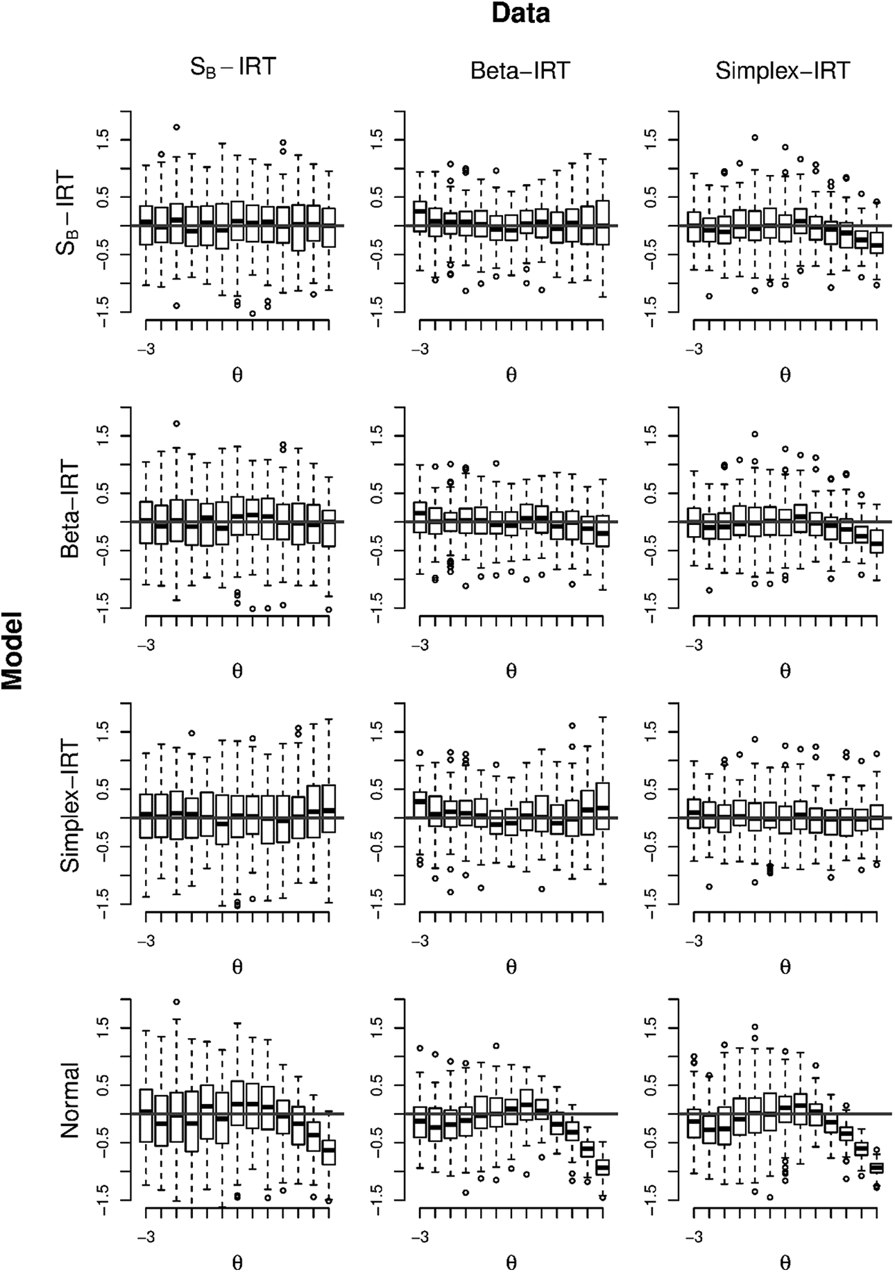
To study the consequences for the person parameters of fitting an incorrect model to the data, we focus on the parameter estimates of ${\text{θ}}_p$ across the different models for the different data scenarios in the simulation study. Figure 10 depicts boxplots of the errors of the person parameters across replications for the different fitted models under the different data generating scenarios for 18 items. As expected due to the above, if the correct model is fit, the boxplots indicate no bias. If the incorrect model is fit, it is most notable that the normal-IRT model is biased, with under estimation of the lower ${\text{θ}}_p$ values and over estimation of the upper ${\text{θ}}_p$ values. In addition, it seems that the S_B -IRT and beta-IRT model are relatively robust with respect to each other. However, if the data are generated according to a simplex-IRT model, the ${\text{θ}}_p$ estimates in both the S_B -IRT and beta-IRT model are biased for the upper ${\text{θ}}_p$ values. In addition, the simplex-IRT model is biased for the lower and upper ${\theta }_p$ values if the data follow a beta-IRT model.

Figure 10.

Boxplots of the errors in ${\mathit{\text{θ}}}_{\text{p}}$ in each model (rows) for the different data generating models (columns) in the simulation study.

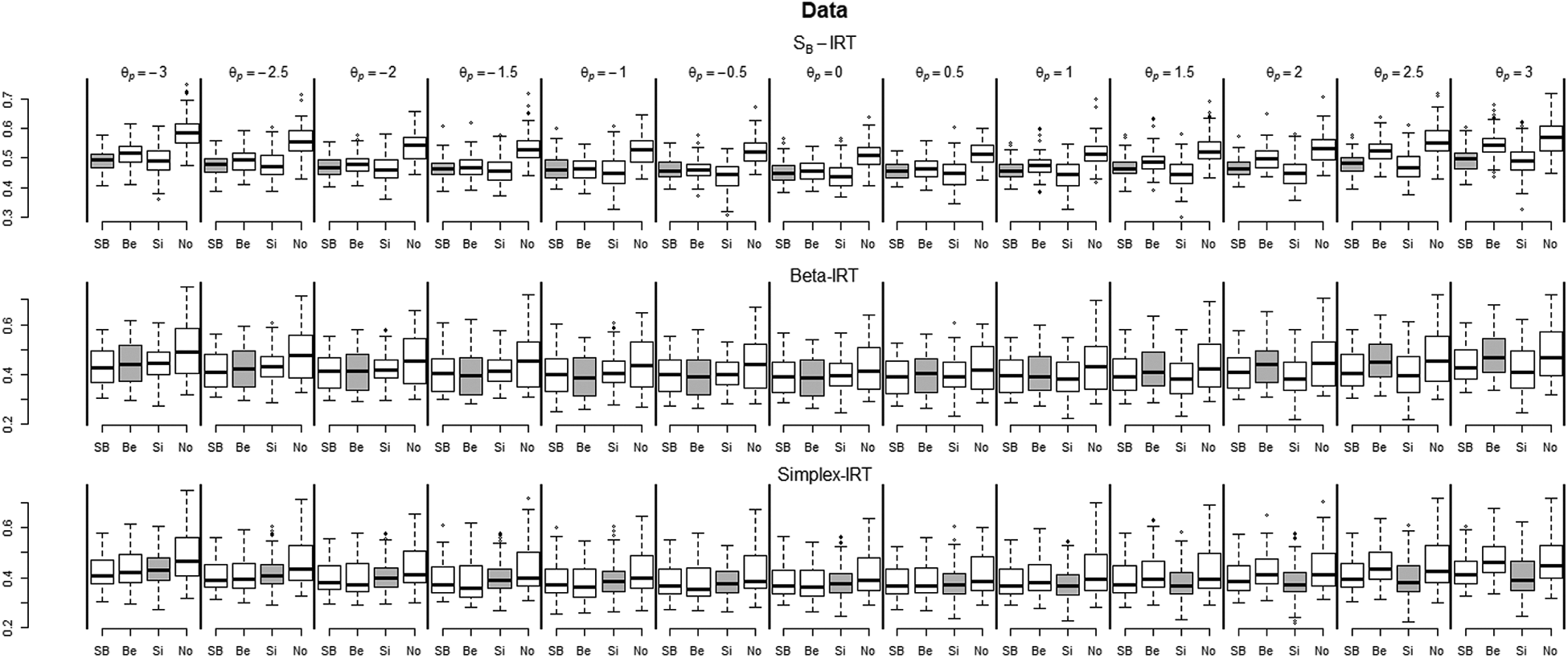
Figure 11 depicts the boxplots of the estimated posterior standard deviations of the person parameters across replications for each true value of ${\text{θ}}_p$ in the different fitted models and under the different data generating scenarios for 18 items. As a reference, the boxes of the estimates in the true model are in gray. As can be seen, the normal-IRT model overestimates the posterior standard deviation under all data generation scenarios with the largest effect for the S_B -IRT data scenario. For the other models, some differences are also evident, but smaller: For instance, in the beta-IRT, the posterior standard deviation is overestimated for larger values of ${\text{θ}}_p$ in the S_B -IRT data scenario. In addition, the S_B -IRT and simplex-IRT underestimate the posterior standard deviation for larger ${\theta }_p$ values in the beta-IRT scenario. Finally, the beta-IRT model overestimates the posterior standard deviation for larger values of ${\text{θ}}_p$ in the simplex scenario. Similarly as above, these local effects in the upper range of ${\text{θ}}_p$ are due to positive skew in the simulated data. If these effects are reversed into negative skew, the lower range of ${\text{θ}}_p$ will be affected.

Figure 11.

Boxplots of the estimated posterior standard deviation of ${\mathit{\text{θ}}}_{\text{p}}$ in each model for each true value of ${\mathit{\text{θ}}}_{\text{p}}$ and for the different data generating models (rows) in the simulation study for 18 items. SB = S_B -IRT; Be = beta-IRT; Si = simplex-IRT; No = normal-IRT; IRT = item response theory.

Conclusion

The person parameter recovery is acceptable in all models. If an incorrect model is fit to the data, the person parameter estimates and posterior standard deviations in a normal-IRT model are biased across the full ${\text{θ}}_p$ range. For the other models, the person parameters and posterior standard deviations may be biased in the upper or lower range of ${\text{θ}}_p$ depending on the estimated model and the properties of the data under the data generation model.

Application

Data

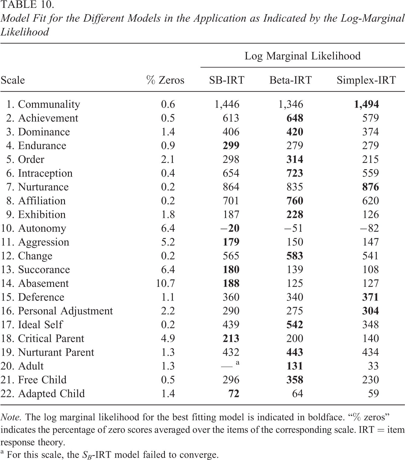
In this application, we apply the zero and one inflated IRT models from the present study to a dataset containing the responses of 244 respondents to 218 items from the ACL (Gough & Heilbrun, 1980) of which two scales were considered above in Motivating Example 1. The ACL is a personality questionnaire consisting of adjectives like “stable,” “responsible,” and “organized” to which respondents indicate to what degree this adjective applies to them. In the present study, the ACL was administered using a continuous response scale consisting of a 60-mm line segment. Responses are scored as the distance (in millimeters) from the left end of the line segment (“totally not applicable to me”). These responses are rescaled into the [0,1] interval to enable application of the present models. The ACL administration considered here covered 22 scales (the original ACL covers 30 scales). All scales contained 10 items, except for the two final scales 21 and 22 which contain nine items. In the ACL data, the upper end point of the response scale is never used. The average percentage of lower end point (zero) scores is between 0.2% and 10.7% (see Table 10).

Table 10.

Model Fit for the Different Models in the Application as Indicated by the Log-Marginal Likelihood

		Log Marginal Likelihood
Scale	% Zeros	SB-IRT	Beta-IRT	Simplex-IRT
1. Communality	0.6	1,446	1,346	1,494
2. Achievement	0.5	613	648	579
3. Dominance	1.4	406	420	374
4. Endurance	0.9	299	279	279
5. Order	2.1	298	314	215
6. Intraception	0.4	654	723	559
7. Nurturance	0.2	864	835	876
8. Affiliation	0.2	701	760	620
9. Exhibition	1.8	187	228	126
10. Autonomy	6.4	−20	−51	−82
11. Aggression	5.2	179	150	147
12. Change	0.2	565	583	541
13. Succorance	6.4	180	139	108
14. Abasement	10.7	188	125	127
15. Deference	1.1	360	340	371
16. Personal Adjustment	2.2	290	275	304
17. Ideal Self	0.2	439	542	348
18. Critical Parent	4.9	213	200	140
19. Nurturant Parent	1.3	432	443	434
20. Adult	1.3	— a	131	33
21. Free Child	0.5	296	358	230
22. Adapted Child	1.4	72	64	59

Note. The log marginal likelihood for the best fitting model is indicated in boldface. “% zeros” indicates the percentage of zero scores averaged over the items of the corresponding scale. IRT = item response theory.

^a For this scale, the S_B -IRT model failed to converge.

Models

The four zero and one inflated IRT models considered in the simulation study are fit to each scale of the ACL separately. Aim is to see which models fit best and how the results from the different models compare to each other. In addition, we fitted the conventional models to see how the results differ. In our MCMC implementation, we used four chains of 10,000 samples from the posterior parameter distribution each. For each chain, the first 5,000 samples are discarded as burn-in. The chains are judged to be converged based on the split R-hat (Vehtari et al., 2021). For one scale, Scale 20 (Nurturant parent), the inflated S_B -IRT model failed to converge with the split R-hat well above 1 for multiple parameters. Therefore, for Scale 20, we omit the results concerning the S_B -IRT model. For the conventional models, we transformed all zero scores to 1e-05 except for the simplex-IRT model as this resulted in divergence of the dispersion parameter. For this model, we transformed the zeros to 0.01.

Results

Table 10 contains the log marginal likelihood for the different bounded-IRT models and the different ACL scales. Note that the log marginal likelihood can also be used to calculate Bayes’s factors. For instance for the Communality scale, the log Bayes’s factor between the S_B -IRT model and the beta-IRT model equals $1446-1346 = 100$ , indicating that evidence is strongly in favor of the S_B -IRT model. Here, however, similarly as in the simulation study, we rely on the log marginal likelihood as a fit statistic, that is, the larger values indicate a better model fit. In addition, the DIC and WAIC fit indices agree about the best fitting model for all scales except Scale 22 (Adapted Child). For this scale, the DIC and WAIC indicate the beta-IRT model as best fitting model, while the log marginal likelihood indicates the S_B -IRT model. As in the results of the simulation study, the log marginal likelihood is associated with overall fewer false positives, and we rely on the log marginal likelihood and conclude that the S_B -IRT model fits best for Scale 22.

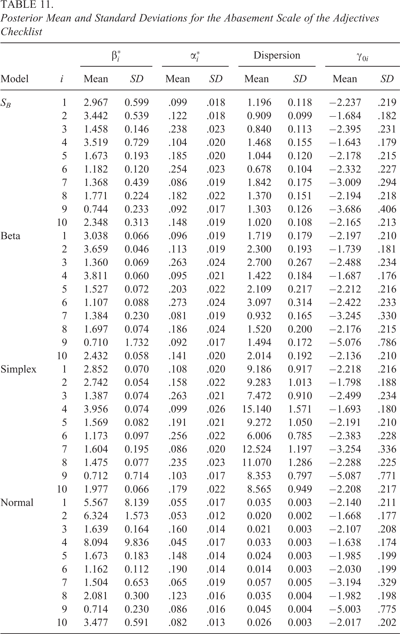
As can be seen in Table 10, the beta-IRT model fits best to the majority of the scales followed by the S_B -IRT model. The simplex-IRT model fits best to three of the 22 scales. Interestingly, the S_B -IRT model fits best to the scales with the higher degrees of zero inflation. Below, we look closer to the results of the “Abasement” scale that was analyzed in the motivating example above and that has the most severe zero inflation on average (10.7%). Table 11 contains the posterior means and standard deviations for the ${\text{α}}_i^{*}$ , ${\text{β}}_i^{*}$ , dispersion, and ${\text{γ}}_{0i}$ parameters across models. Note that ${\text{α}}_i^{*}$ and ${\text{β}}_i^{*}$ are transformed parameters, which can be compared across the different models. In addition, ${\text{γ}}_{1i}$ are not considered as there are no one responses in the data. As can be seen from the table, results differ most notably between the normal-IRT model and the bounded-IRT models with the posterior means for ${\text{β}}_i^{*}$ being systematically higher and ${\text{α}}_i^{*}$ being systematically smaller for the normal-IRT model. The posterior means and standard deviations for the bounded-IRT models differ minorly for some items, but in general, the results tend to converge for the item parameters.

Table 11.

Posterior Mean and Standard Deviations for the Abasement Scale of the Adjectives Checklist

		${\text{β}}_i^{*}$		${\text{α}}_i^{*}$		Dispersion		${\text{γ}}_{0i}$
Model	i	Mean	SD	Mean	SD	Mean	SD	Mean	SD
SB	1	2.967	0.599	.099	.018	1.196	0.118	−2.237	.219
	2	3.442	0.539	.122	.018	0.909	0.099	−1.684	.182
	3	1.458	0.146	.238	.023	0.840	0.113	−2.395	.231
	4	3.519	0.729	.104	.020	1.468	0.155	−1.643	.179
	5	1.673	0.193	.185	.020	1.044	0.120	−2.178	.215
	6	1.182	0.120	.254	.023	0.678	0.104	−2.332	.227
	7	1.368	0.439	.086	.019	1.842	0.175	−3.009	.294
	8	1.771	0.224	.182	.022	1.370	0.151	−2.194	.218
	9	0.744	0.233	.092	.017	1.303	0.126	−3.686	.406
	10	2.348	0.313	.148	.019	1.020	0.108	−2.165	.213
Beta	1	3.038	0.066	.096	.019	1.719	0.179	−2.197	.210
	2	3.659	0.046	.113	.019	2.300	0.193	−1.739	.181
	3	1.360	0.069	.263	.024	2.700	0.267	−2.488	.234
	4	3.811	0.060	.095	.021	1.422	0.184	−1.687	.176
	5	1.527	0.072	.203	.022	2.109	0.217	−2.212	.216
	6	1.107	0.088	.273	.024	3.097	0.314	−2.422	.233
	7	1.384	0.230	.081	.019	0.932	0.165	−3.245	.330
	8	1.697	0.074	.186	.024	1.520	0.200	−2.176	.215
	9	0.710	1.732	.092	.017	1.494	0.172	−5.076	.786
	10	2.432	0.058	.141	.020	2.014	0.192	−2.136	.210
Simplex	1	2.852	0.070	.108	.020	9.186	0.917	−2.218	.216
	2	2.742	0.054	.158	.022	9.283	1.013	−1.798	.188
	3	1.387	0.074	.263	.021	7.472	0.910	−2.499	.234
	4	3.956	0.074	.099	.026	15.140	1.571	−1.693	.180
	5	1.569	0.082	.191	.021	9.272	1.050	−2.191	.210
	6	1.173	0.097	.256	.022	6.006	0.785	−2.383	.228
	7	1.604	0.195	.086	.020	12.524	1.197	−3.254	.336
	8	1.475	0.077	.235	.023	11.070	1.286	−2.288	.225
	9	0.712	0.714	.103	.017	8.353	0.797	−5.087	.771
	10	1.977	0.066	.179	.022	8.565	0.949	−2.208	.217
Normal	1	5.567	8.139	.055	.017	0.035	0.003	−2.140	.211
	2	6.324	1.573	.053	.012	0.020	0.002	−1.668	.177
	3	1.639	0.164	.160	.014	0.021	0.003	−2.107	.208
	4	8.094	9.836	.045	.017	0.033	0.003	−1.638	.174
	5	1.673	0.183	.148	.014	0.024	0.003	−1.985	.199
	6	1.162	0.112	.190	.014	0.014	0.003	−2.030	.199
	7	1.504	0.653	.065	.019	0.057	0.005	−3.194	.329
	8	2.081	0.300	.123	.016	0.035	0.004	−1.982	.198
	9	0.714	0.230	.086	.016	0.045	0.004	−5.003	.775
	10	3.477	0.591	.082	.013	0.026	0.003	−2.017	.202

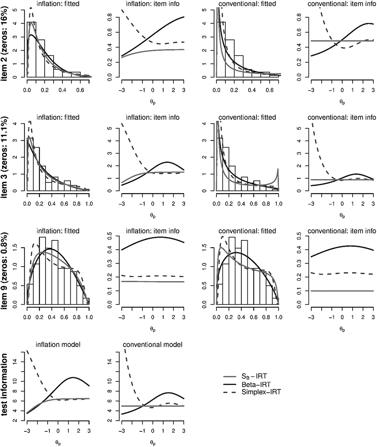
Figure 12 contains histograms with fitted curves and item information for the zero-one inflated IRT models and the conventional bounded IRT models for three example items (2, 3, and 9) from the Abasement scale. As can be seen, generally, the information is larger in the inflation IRT model. In addition, the fitted curves differ notably across the inflation IRT models and the conventional models, especially in the case of a higher percentage of zero scores in the item.

Figure 12.

First three rows: Histograms with fitted curves and item information for the zero-one inflated item response theory (IRT) models and the conventional bounded IRT models for three example items (2, 3, and 9) from the Abasement scale. Fourth row: Test information functions.

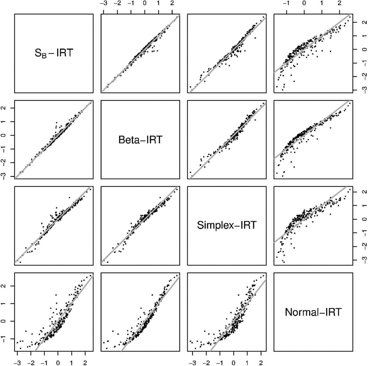
Figure 13 depicts the posterior means of ${\text{θ}}_p$ of the Abasement scale for the four different models. As can be seen, for the normal-IRT model, these estimates differ substantially from the others especially in the upper and lower range of ${\text{θ}}_p$ . In addition, for the S_B -IRT and beta-IRT model, the posterior mean estimates are almost perfectly related, while for the simplex-IRT model, some minor differences are notable in the upper and lower range of ${\text{θ}}_p$ .

Figure 13.

Posterior mean estimates of ${\mathit{\text{θ}}}_{\text{p}}$ for the Abasement scale.

Discussion

In this study, we proposed a zero and one inflated IRT framework for bounded continuous data in the closed interval. In two motivating examples, we showed in both real and simulated data that not taking zero and one inflation into account can seriously distort modeling results. Next, in the simulation study, we demonstrated the viability of the proposed framework and the suitability of the log marginal likelihood to select among the different models, even in small sample sizes. In addition, we studied the consequences of misfit in the distribution assumed by the continuous IRT models. It turned out that not modeling the bounded nature of the data can result in severe bias in the posterior means and standard deviations of the person and item parameters, but that misspecification of the bounded IRT model generally has a smaller impact on the results. Therefore, in practice, a general advice is to use the simplex-IRT model if (some of) the items show bimodality (as this model is most flexible in these cases) and to use the beta-IRT and S_B models in the case of unimodal data (as these models are more flexible in these cases, although these models can handle some degree of bimodality). In addition, as misfit may still bias the results depending on the data generating model and the parameters of interest, it is always advisable to test different models and to base inferences on the best fitting model to decrease the misfit to a minimum.

Although we thus argue for avoiding misfit of the conditional response distribution in practical applications involving bounded continuous data, the present methodology is fully parametric, so that there will always be some misfit. An alternative may be a nonparametric approach (e.g., based on splines, Jungbacker et al., 2014) or an approach based on mixtures (e.g., Dolan & Van der Maas, 1998); however, in these more complex models, more parameter uncertainty is introduced. Therefore, we emphasized the model fit and model selection aspect of the present topic, to hopefully decrease misfit while retaining the benefits from the parametric form of the distribution. To this end, further research may focus on item specific distributions (e.g., the beta distribution for some of the items and the S_B distribution for others) and other distributional forms. For instance, Smithson and Shou (2017; see also Shou & Smithson, 2019) proposed the family of CDF-quantile distributions for bounded continuous variables. Although we are not aware of implementations in an IRT or factor analysis framework, these distributions are promising as they have shown to be more flexible than the beta distribution for instance.