
Abstract
The social relations model (SRM) is very often used in psychology to examine the components, determinants, and consequences of interpersonal judgments and behaviors that arise in social groups. The standard SRM was developed to analyze cross-sectional data. Based on a recently suggested integration of the SRM with structural equation models (SEM) framework, we show here how longitudinal SRM data can be analyzed using the SR-SEM. Two examples are presented to illustrate the model, and we also present the results of a small simulation study comparing the SR-SEM approach to a two-step approach. Altogether, the SR-SEM has a number of advantages compared to earlier suggestions for analyzing longitudinal SRM data, making it extremely useful for applied research.
Keywords
The social relations model (SRM) is a mathematical approach that allows for investigating the processes underlying interpersonal perceptions, interpersonal judgments, and interpersonal behaviors. It is used in a number of psychological and nonpsychological disciplines, including personality and social psychology, educational psychology, clinical psychology, political science, and anthropology, to disentangle the components that underlie interpersonal phenomena. For example, social and personality psychologists use the SRM to better understand liking between unacquainted individuals (e.g., Küfner et al., 2012; Leckelt et al., 2015; Salazar-Kämpf et al., 2018). Clinical psychologists have used the model to investigate interpersonal processes in group psychotherapy (e.g., Christensen & Feeney, 2016), and educational psychologists have examined students’ performance in learning groups to determine which students profit the most from such groups (e.g., Horn et al., 1998).
In most applications to date, the SRM is used with cross-sectional data (see Kenny, 1994, 2019, for an overview and references regarding usage of the SRM). However, due to increased interest among applied researchers in how interpersonal phenomena develop over time, there is also growing interest in how longitudinal data can be analyzed with the SRM. This tendency is corroborated by technical developments such as smartphone apps or online diaries that allow for the economical measurement of SRM data. Personality psychologists, for example, are interested in how liking changes as individuals become acquainted with each other and how these changes can be explained (see, e.g., Leckelt et al., 2015; Salazar-Kämpf et al., 2018). They also investigate whether low perceptions of others in terms of self-confidence or assertiveness go along with increases in assertiveness reputations over time (Rau et al., 2019).
So far, there are only a few recommendations for applied researchers on how to analyze longitudinal SRM data (e.g., Gill & Swartz, 2007; Nestler, 2018; Nestler et al., 2017; Park & Flink, 1989). Here, we show how the recently suggested combination of the SRM with structural equation models (SR-SEM, Nestler et al., 2020), which allows researchers to model the relations among multivariate SRM data in a very flexible way, can be used to implement an autoregressive path model and a linear growth model for longitudinal SRM data. We also explain how the two models’ parameters can be interpreted. These models are routinely used by applied researchers for analyzing traditional longitudinal panel data and will allow applied SRM researchers to investigate a number of interesting research questions. For instance, researchers can use the models to examine questions of stability and change in SRM components (e.g., what components of interpersonal judgments change over time) and whether certain variables affect these changes.
The present article is organized as follows: We begin with a description of the SRM and the design used to collect SRM data (i.e., the round-robin design). We then proceed to a description of the approaches that are currently used to analyze longitudinal round-robin data. Thereafter, we describe the SR-SEM and show how an autoregressive SR-SEM and a growth model SR-SEM can be implemented in this framework. We then present the results of a illustrative data example for the autoregressive SR-SEM and the results of a illustrative data example for the linear growth model. Finally, we describe the results of a small simulation study.
The SRM and the Round-Robin Design
Imagine that you have asked a group of first-year university students to judge each other in terms of liking. A design in which every individual within a group judges all other group members in terms of a single variable (such as liking) is called a round-robin design, and the resulting data are called round-robin data (e.g., Kenny, 1994; Kenny et al., 2006; Lüdtke et al., 2013; Nestler, 2018; Nestler et al., 2015). An important feature of this type of data is that each individual serves both as a perceiver who judges all other individuals and as a target who is judged by all others in the group. Thus, the round-robin design provides dyadic data, with two judgments for each dyad available: i’s judgment of j and j’s judgment of i.
The (cross-sectional) univariate SRM can be used to analyze data stemming from such a round-robin design. According to the model (see Kenny, 1994; Kenny et al., 2006, for an overview), person i’s judgment of person j can be written as

where
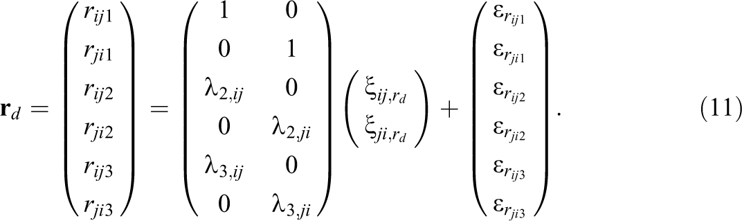
As mentioned, the round-robin design generates two judgments for the same specific dyad d. When we write these two judgments in vector form

one can see that the round-robin judgments contain information about the perceiver effect and the target effect for a specific person (e.g., person i) and the two relationship effects of a specific dyad. This allows the variance of the two person-level effects as well as their covariance to be estimated. Furthermore, one can estimate the variance of the relationship effects and the covariance between the two relationship effects.
The perceiver variance
Warner et al. (1979) suggested that the analysis of variance (ANOVA) approach can be used to estimate the SRM variance and covariance model parameters (see also Bond et al., 1997; Bond & Lashley, 1996). However, the ANOVA method has some limitations (see Lüdtke et al., 2013; Snijders & Bosker, 2012, for thorough discussions). This has led to the development of alternative estimation approaches such as maximum likelihood (ML; Gill & Swartz, 2007; Nestler, 2016, 2018) or a Bayesian approach (Gill & Swartz, 2007; Lüdtke et al., 2013). An advantage of the latter two approaches is that they can be applied to more complex models (e.g., longitudinal round-robin data). The parameters of the SR-SEM, for example, are estimated with an ML approach (Nestler et al., 2020).
Earlier Approaches to Longitudinal SRM Data
In the previous section, we described the cross-sectional SRM. However, researchers have very often assessed longitudinal round-robin data. For instance, in one of the studies we use below to illustrate the SR-SEM (see Illustrative Data Example I), participants were randomly assigned to small groups. These groups then took part in three sessions that were each 1 week apart. In each session, each group member was asked to rate every other group member and was also rated by every other group member with regard to how agentic they are (i.e., their ability to be a good group leader). Thus, we have data for a round-robin variable at three time points. How would an applied SRM researcher currently examine such longitudinal round-robin data? Three approaches have been used or suggested (see also Nestler et al., 2017, for a similar discussion): using multiple cross-sectional SRMs (e.g., Gill & Swartz, 2007; Hoff, 2005), a two-step approach in which time-point-specific SRM effects are estimated and then used in standard longitudinal models (e.g., Küfner et al., 2012; Leckelt et al., 2015), and the social relations growth model (Nestler et al., 2017). Below, we discuss the limitations of these three approaches.
Multiple cross-sectional SRMs
The idea behind this (quite limited) approach is to compute the SRM variance and covariance parameters at each time point and for each round-robin group (see Park & Flink, 1989). In our example, for instance, a researcher would have to compute the actor or partner effect variance for each of the round-robin groups at each of the three time points. The resulting (cross-sectional) SRM parameter estimates are then compared across occasions with a linear regression model such as the ANOVA or a t test. We think that this approach is problematic because ultimately the method’s unit of analysis is the round-robin group. Hence, it cannot be applied when only one round-robin group is assessed. Moreover, the performance of the second-stage statistical methods will be problematic when the number of groups is small. Finally, this approach cannot be used to model longitudinal trajectories in the SRM effects or between-person or between-dyad differences in these trajectories.
Two-step approach
This approach uses cross-sectional SRMs to estimate individual-level or dyad-level SRM effects for each time point. Thereafter, the time-point-specific effects are used in standard longitudinal models such as a growth model or an autoregressive model to examine the respective research question (see Küfner et al., 2012; Leckelt et al., 2015; Nestler et al., 2015; van Zalk & Denissen, 2015, for an application). In our example, a researcher may have estimated the target effects at each of the three time points and entered these effects into an autoregressive panel model in the second step of the analyses. Although intuitively appealing, this approach assumes that the first-step estimates (e.g., the estimated target effect of person i) are error-free measures of their true population parameters (e.g., the true target effect of person i). However, this assumption is problematic for standard error calculations, especially when the number of round-robin group members is small (see Lüdtke, Robitzsch, & Trautwein, 2018; Nestler et al., 2015). For instance, simulation studies show that a two-step approach yields unacceptable coverage rates when there are only a few round-robin group members (Nestler et al., 2017, 2020). Furthermore, the two-step approach parameter estimates are substantially biased in such situations.
Social relations growth model
Finally, the social relations growth model (see Nestler et al., 2017) is based on a combination of the SRM with a longitudinal mixed model (e.g., Verbeke & Molenberghs, 2009). The social relations growth model includes a time variable that predicts the repeated round-robin judgments within each dyad. Thus, if person i has judged person j at three measurement occasions, the social relations growth model would predict these three judgments via a time variable used to code the three time points. The intercept and the slope of the time variable are assumed to contain a perceiver effect, a target effect, and a relationship effect. The social relations growth model thus assumes that the round-robin judgment of dyad
To summarize, the methods used so far are either statistically questionable or very limited in terms of the questions that can be investigated with them. We think this last point is particularly important because applied SRM researchers can be (and are) interested in very different things depending on the discipline in which they are working. For example, SRM researchers investigate whether perceiver effects are predictive of target effects measured at later time points (e.g., whether perceiving others as low on agency is longitudinally associated with a higher agency reputation oneself; see Rau et al., 2019), whether the relationship effects of a round-robin variable are stable over time and/or whether i’s unique perception of j predicts j’s unique perception of i at a later time point (i.e., longitudinal dyadic reciprocity; Salazar-Kämpf et al., 2018). They are also interested in whether and if so how the SRM effects of a round-robin variable change over time, and when several round-robin variables for a construct have been measured at each time point, whether the SRM effect factor in a factor model is invariant over time (measurement invariance; see, e.g., Srivastava et al., 2010). Finally, they might also be interested in defining a growth model for these SRM effect factors.
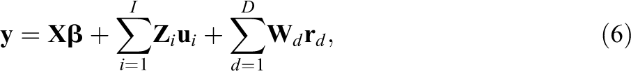
This discussion shows that a new approach to analyzing longitudinal round-robin data has to be very flexible in order to investigate all of these different questions. If the longitudinal data were not (dyadic) round-robin data, one could use a longitudinal SEM (see Grimm et al., 2017; Little, 2013; Mund & Nestler, 2019; Singer & Willett, 2003), because it allows for estimating a plethora of different longitudinal models within a single modeling framework. In the longitudinal SEM, a person’s observed scores
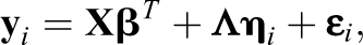

where
The mathematical reason for the flexibility of the longitudinal SEM is that it acknowledges that every longitudinal model is associated with different assumptions regarding the mean structure
However, SRM researchers do not have data from individual persons, but rather dyadic round-robin data, and they would be able to take advantage of the flexibility of the SEM if they could analyze their longitudinal round-robin data by combining the SRM with the SEM framework. In such a case, by appropriately specifying the model matrices, any set of theoretical assumptions about the longitudinal course of the SRM effects could be investigated and tested.
SR-SEM: A Combination of the SRM and SEM
In fact, Nestler et al. (2020) recently proposed a combination of the SRM with the SEM (which they termed the SR-SEM). However, in this technical article, they introduce the model in very general terms and only show how to estimate the model parameters using an ML estimator. They do not show how to use the SR-SEM to examine longitudinal round-robin data, although this would be very interesting from a methodological and applied perspective, because modeling such data poses a number of specific challenges. For instance, it is not immediately clear how one should specify the mean structure in an SR-SEM growth model, since round-robin judgments include random effects at different levels. Moreover, it is difficult to determine which parameters to constrain to the same value and also how to interpret the parameters. To fill this gap, we first describe the SR-SEM and then introduce and explain SR-SEM versions of the aforementioned two longitudinal models. We restrict ourselves to these two models because they are very often used to model longitudinal data; our expositions will thus allow researchers to investigate a number of interesting research questions. Moreover, the description of both models allows us to illustrate the specific challenges that occur when one models longitudinal round-robin data and we hope that they are good showcases enabling researchers to implement and interpret the parameters of other SR-SEM longitudinal data models.
Nestler et al. (2020) describe a combination of a multivariate SRM with the SEM that allows for modeling linear relationships between the (latent) perceiver effects and target effects of different round-robin variables or the (latent) relationship effects of these variables. The foundation for this combined model is to write the multivariate round-robin judgment vector
where
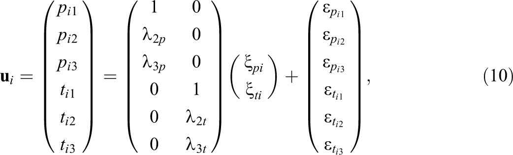
For the person effects,
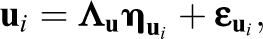

where
A similar model is defined for the dyad effects:

where
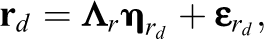
To illustrate the model, we focus on one dyad

where, for example,
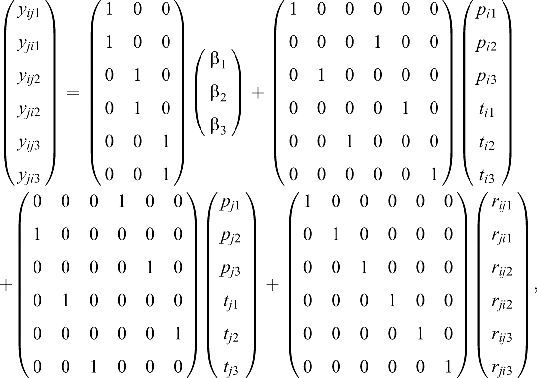
Furthermore, when we assume that all the individual-level SRM effects are indicators of one latent perceiver and one target effect factor, respectively, Equation 7 for Person i is
where
Again, we set
SR-SEMs for Longitudinal SRM Data
Having introduced the SR-SEM, we now turn to a description of an autoregressive path model variant of the SR-SEM and a linear growth model for longitudinal SRM Data. Our descriptions are meant as illustrations and show how researchers can specify (two commonly used) longitudinal models for SRM data within the SR-SEM framework. We also explain how these models’ parameters can be interpreted. Below, we assume that one round-robin variable was assessed at NT time points. Thus, the number of round-robin measures K equals NT . We will return to models in which K variables were assessed at each measurement occasion later in the General Discussion.
Autoregressive SR-SEM
The autoregressive SR-SEM for the person effects can be obtained by setting
where bp
and bt
are the autoregressive parameters for the perceiver effects and target effects, respectively.
A very similar model can be specified for the dyad-level effects. The only difference between the structural coefficient matrix
Here, br
is the autoregressive parameter. In our example, a positive parameter would indicate that the unique agency perceptions between two time points are correlated.
In addition to the structural coefficient matrices, the autoregressive SR-SEM requires that
Similar to the standard autoregressive path model, the variance and covariance terms at later time points (e.g., Time Point 2 and 3) are residual variance and covariance terms and can be forced to the same value-across and within time points-in a real data application.
Linear growth SR-SEM
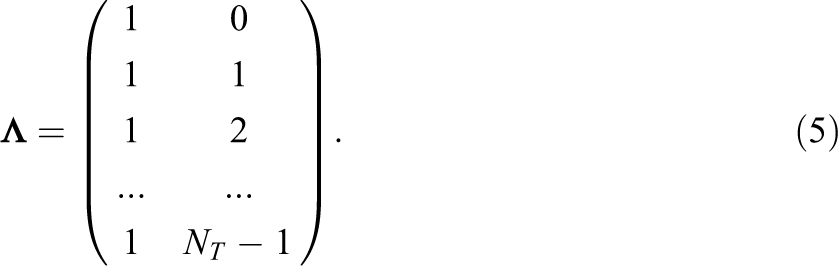
Here, we use a linear latent growth model for the person-level and dyad-level effects to show how a latent growth model for SRM data can be defined. To this end, we set
We are thus defining four latent person-level factors (i.e.,
As in the case of a standard linear growth model, the covariance matrix of
where
For the dyad-level effects, we also define a linear growth model by setting
Again, the covariance matrix
Here,
Mean and covariance structure of the models
The definition of the model matrices can be used to determine the covariance structure and the mean structure of the autoregressive SR-SEM or the linear growth SR-SEM (see Equation 18), respectively (see the next section). However, with regard to the mean structure, two points are important to consider. First, the effect of person-level and dyad-level covariates can be examined by including these covariates in Equation 7 and/or Equation 8 and estimating
Estimation of the Model’s Parameters
When the model matrices have been defined in the appropriate way, the mean and the covariance structure of the longitudinal SR-SEM are given by (see Nestler et al., 2020)
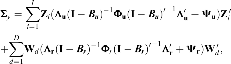

If we assume that
The log-likelihood of the data given the parameter vector

whereby the covariance matrix and expectations are functions of the unknown parameter vector
Illustration I: An Autoregressive SR-SEM
We illustrate the suggested SR-SEM approach to longitudinal round-robin data with two examples. In the first example, we use an autoregressive SR-SEM to model the sample data we mentioned at the start of this article. We have chosen to use the autoregressive SR-SEM for this illustration because the round-robin data were collected over a period of 3 weeks; estimating the linear growth SR-SEM for this data is thus not meaningful. In the second example, we estimate a linear growth SR-SEM for the CONNECT data set that was also used in Nestler et al. (2017).
Data and Data Analysis
The data for this example stem from a longitudinal, laboratory round-robin study called Personality Interaction Laboratory Study (see Geukes et al., 2019) in which participants were assigned to round-robin groups consisting of four to six individuals each. Each round-robin group took part in three laboratory sessions that were each 1 week apart. Here, we use the data of G = 20 round-robin groups to illustrate the autoregressive SR-SEM (N = 114).
At the start of each session, the group members were asked to judge the other group members and were also judged by the other group members with regard to 10 interpersonal perception items including, for example, liking, trustworthiness, or assertiveness (see Geukes et al., 2019). Here, we use the ratings for whether the other group members are good group leaders (“I can imagine this person as a good leader”). This item, as well as all other items, had to be answered on a scale ranging from 1 (does not apply at all) to 6 (applies perfectly). Note that in personality psychology, the item would be taken as a measure of an individual’s success regarding the motive of getting ahead or agency. This is how we interpreted the leadership perceptions in the prior section, and we will stick to this interpretation in what follows (see Rau et al., 2019).
These initial ratings were followed by two to three social interaction tasks. For example, in the first session, groups were asked to introduce themselves in detail, while in the second session, the group was asked to complete the “Lost on the Moon” task, in which they have to correctly prioritize a list of items in terms of how helpful they would be for survival on the moon after a crash landing. After each of these tasks, participants were again asked to provide leadership ratings. Across the three sessions, 10 “waves” of round-robin data were available (i.e., four waves in Session 1, three waves in Session 2, and another four waves in Session 3).
To reduce model complexity, we aggregated all waves from the same session, so that the autoregressive SR-SEM comprises data from three time points. Specifically, a model was defined in which the perceiver and target effects at Time Point 2 were regressed on the perceiver and target effects at Time Point 1, and the perceiver and target effects at Time Point 3 were regressed on the perceiver and target effects at Time Point 2 (see Equation 12). Following the standard autoregressive SEM approach, the respective autoregressive parameters and cross-lag parameters were constrained to be equal over time. We also forced the variance of the perceiver effects, the variance of the target effects, or their covariance at the second and the third time point to the same value over time (see Equation 14). The same model was specified for the relationship effects.
We used the srm package to obtain the ML parameter estimates. For comparison, we also estimated the parameters using a two-step approach. To this end, we estimated the perceiver effects, target effects, and relationship effects of the three round-robin variables using TripleR (Schönbrodt et al., 2017). The person-level and dyad-level effects were then used as variables in the lavaan package (Rosseel, 2012). The study’s multiple round-robin group design would allow us to investigate whether the average level of leadership ratings varies across groups. However, differences between groups are usually not of great interest to SRM researchers. We therefore removed the group effects by group-mean centering the data prior to the analyses (see Lüdtke et al., 2013; Nestler, 2016). The R code and the data can be downloaded from the OSF (https://osf.io/dvnqj/).
Results
Table 1 shows the autoregressive and cross-lag parameter estimates obtained with the autoregressive SR-SEM and the two-step approach. As can be seen, the estimates of the two approaches were very similar. In both cases, the perceiver effects and target effects were stable over time. Furthermore, in both approaches, we find that the perceiver effects are negatively related with the target effects over time. This indicates that perceiving others as low in agency at a prior time point is associated with being perceived as more agentic at a later time point. However, while the coefficient was significantly different from zero for the two-step approach, this was not so for the autoregressive SR-SEM (
Selected Results of the Autoregressive SR-SEM for the Illustrative Data Example
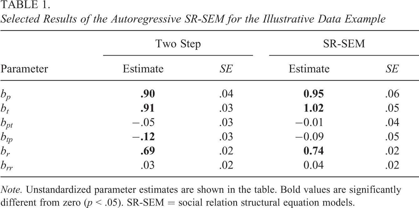
Note. Unstandardized parameter estimates are shown in the table. Bold values are significantly different from zero (p < .05). SR-SEM = social relation structural equation models.
Illustration II: A Linear Growth SR-SEM
The second illustration uses data from the CONNECT study (see Geukes et al., 2019) and was also used in Nestler et al. (2017) to illustrate the social relations growth model. Here, we use this data to demonstrate a linear growth SR-SEM.
Data and Data Analysis
In the CONNECT study, data from 131 first-year university students in psychology were assessed. All 131 students formed one single round-robin group. At 21 measurement occasions during the first semester, each student indicated how much they liked each of the other students (on a scale ranging from 1 = unlikable to 11 = likable; see Geukes et al., 2019, for a description of the full study and further ratings). For the present illustration, following Nestler et al. (2017), we used only the judgments from four of the measurement occasions (Time Points 3, 4, 11, and 19) and we reduced the data to a random subsample of 40 students. That is, the final data set used here is one single round robin group that consists of 40 individuals and contains
The covariance matrix of the growth factors for the individual-level effects and relationship effects was specified as described in Equations 16 and 18, respectively. Furthermore, we also forced the variance of the residual terms of the perceiver effects, of the target effects, and their covariance to the same value over time. The same specification was implemented for the relationship effects. As in the first illustration, we used the srm package to obtain the ML parameter estimates. For the two-step approach, we used TripleR to estimate the perceiver effects, the target effects, and the relationship effects of the round-robin ratings at each time point. We then used these variables as indicators in a latent growth model which we estimated with the lavaan package.
The data set contains missing values (of the 6,240 possible liking judgments, 1,243 were missing). This poses a problem for TripleR, because only a specific number of judgments are allowed to be missing in order to estimate individual level and dyadic effects. Therefore, we decided to generate 20 imputed data sets using the chained equations approach in the mice package (van Buuren & Groothuis-Oudshoorn, 2011). Specifically, the four rating variables were imputed by predictive mean matching and linear regression. For each time point, the ratings at other time points were used as predictor variables. Moreover, to approximately reflect the structure of the round-robin design in the imputations, aggregated means of ratings for each actor and each partner at each time point were computed and included as further predictors in the imputation model (Lüdtke et al., 2017). Thirty iterations were used in the imputation procedure. We evaluated each of the imputed data sets using the procedure described above and then summarized the results using Rubin’s rules. Please note, that for the latent growth model SR-SEM, missing values are not problematic because it is a full-information ML approach that allows for missing data in the round-robin variables. However, since we are interested here in comparing the two-step approach with the SR-SEM, we also fitted the growth SR-SEM to each of the imputed data sets and report the aggregated results that we obtained using Rubin’s rules. Again, the R code and the data can be downloaded from the OSF (https://osf.io/dvnqj/). The OSF project also contains the results for the SR-SEM fitted with full-information ML.
Results
Table 2 shows the results of the two approaches. The estimates in the two-step approach were lower than the estimates in the linear growth SR-SEM, but when we standardize the covariance terms, the results were very similar. In both models, we found that the variance of the perceiver effects at the first time point is larger than the variance of the target effects. The correlation between the two effects at the first time point is small to moderate (r = .18 or r = .14), indicating that students who liked others more on average at the first time point were also liked more on average at the first time point. Furthermore, the variance of the slope factor is higher for the perceiver effects than for the target effects. The covariance between the perceiver intercept effects and perceiver slope effects,
With regard to the relationship effects, we found that they were positively correlated at the first time point (the respective correlation was r = .36 or r = .32). Furthermore, there was a positive correlation between the relationship components of the two slope factors (i.e., r = .19 or r = .21), indicating that changes in the unique liking of dyad
Selected Results for the Linear Growth SR-SEM
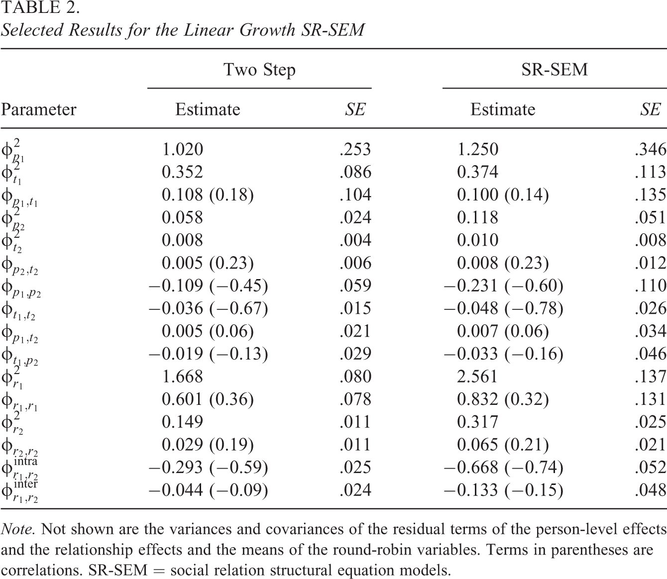
Note. Not shown are the variances and covariances of the residual terms of the person-level effects and the relationship effects and the means of the round-robin variables. Terms in parentheses are correlations. SR-SEM = social relation structural equation models.
Simulation Study
We also conducted a small simulation study to evaluate the statistical properties of the SR-SEM approach for longitudinal round-robin data. To this end, we compared the performance of the ML approach with the two-step approach for estimating the parameters of an autoregressive SR-SEM with different numbers of round-robin groups and different numbers of round-robin group members.
Population Model and Simulation Conditions
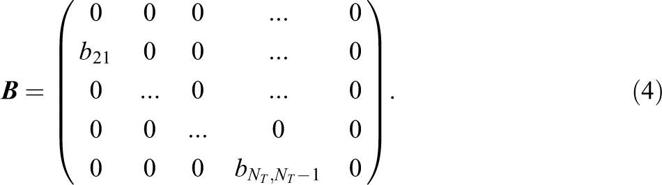
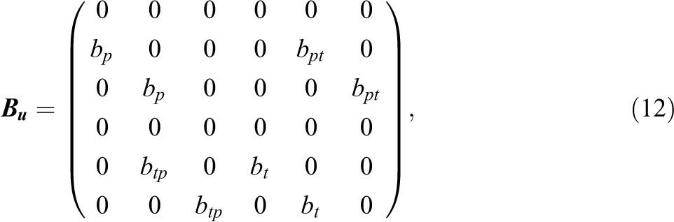
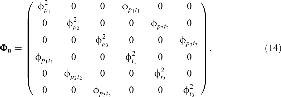
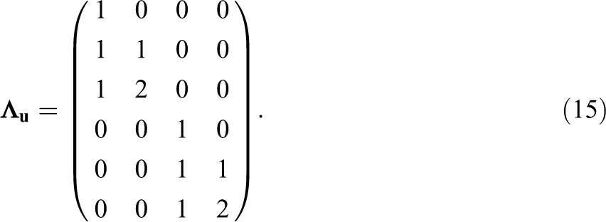
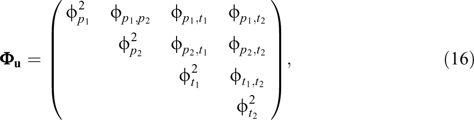
We simulated an autoregressive SR-SEM model in which we assumed that the perceiver effects and the target effects are related over time (i.e., they are somewhat stable). Furthermore, the perceiver effects at Time Point T were assumed to be predictive of the target effects at time T + 1. By contrast, the perceiver effects were assumed to be unrelated to the target effects over time. For the person-level effects and three time points, the model matrices were set to the following values:
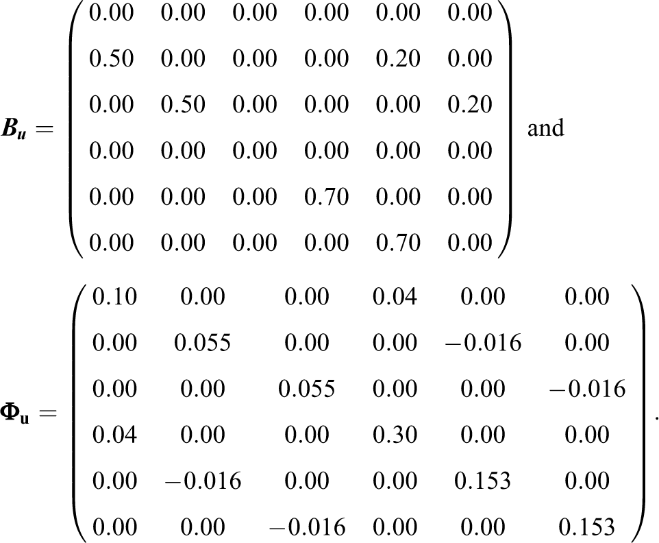
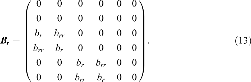
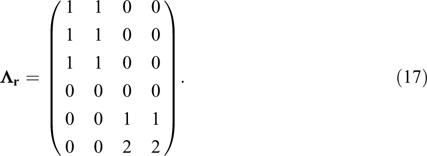
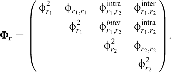
Note, that in the case of the autoregressive SR-SEM, all other matrices and vectors are either identity matrices or are defined to be zero. The matrices for the dyad-level effects were defined in a very similar way:
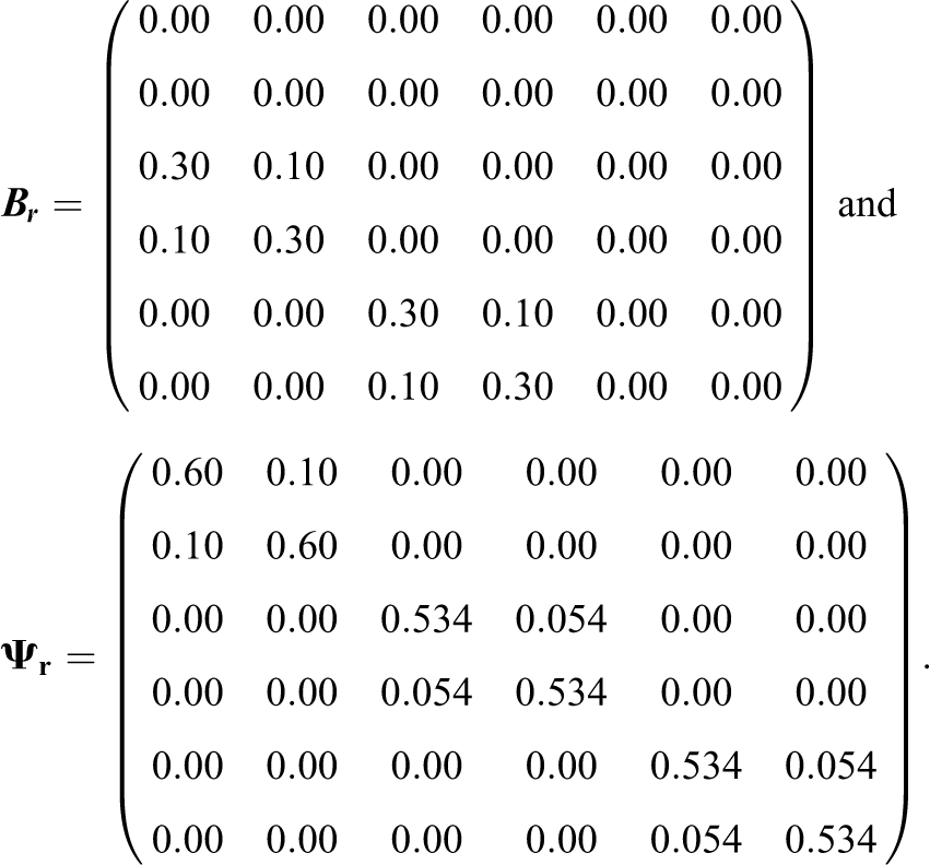
Since there are only a few applications that can be used to select the population parameters, our choice of population parameters was based in part on the results of the first illustrative data example. Furthermore, we used previous applied cross-sectional SRM research to inform the specification of the population parameters. For instance, the variance of the individual-level effects is typically lower than the variance of the dyad-level effects or the perceiver and target effects and the relationship effects are typically positively correlated. We therefore, for example, set the variance of the latent relationship factors and their covariance at the first time point to 0.60 and 0.10 (implying a correlation of about .15). Furthermore, research shows that both perceiver and target effects are stable over time (Kenny, 1994, 2019), that target effects (perceiver effects) predict perceiver effects (target effects, see Rau et al., 2019), and that relationship effects are also stable (see Salazar-Kämpf et al., 2018). Finally, we set some model parameters (e.g., covariance parameters) to negative values or zero to more specifically test the performance of the estimation algorithm.
Besides estimating the model parameters with the two approaches, we manipulated the number of round-robin groups, the number of round-robin group members, and the number of time points. Specifically, the number of round-robin groups was either 15 or 30, the number of round-robin group members was either five or 10, and the number of time points was two, three, or five. For each of the 12 simulation conditions, 1,000 samples were drawn from the population.
Estimators
The model parameters were estimated using the ML approach for the SR-SEM parameters as implemented in the srm package. For the two-step approach, we first estimated the perceiver effects, target effects, and relationship effects of round-robin variables using the ANOVA approach as implemented in the R package TripleR (Schönbrodt et al., 2017). Thereafter, we fitted the resulting model with the ML estimator for SEMs with the lavaan package.
Dependent Measures
The percentage bias of the parameter estimates, the root mean square error (RMSE), and the coverage rate were used to investigate the performance of the two approaches. To decrease the influence of extreme parameter estimates, we computed a robust average measure for bias (i.e., the median). For the robust RMSE, we first computed a robust standard deviation of the parameter estimates in a simulation condition (i.e., the median and the median absolute deviation). The robust RMSE was then obtained by taking the square root of the sum of the squared robust bias and the square of the robust standard deviation. Finally, the observed coverage of the 95% confidence intervals was determined by computing the confidence interval with the standard error of the estimate in each replication. The coverage was then coded 1 if the true parameter value was included in the interval and 0 if the true parameter was not.
Results
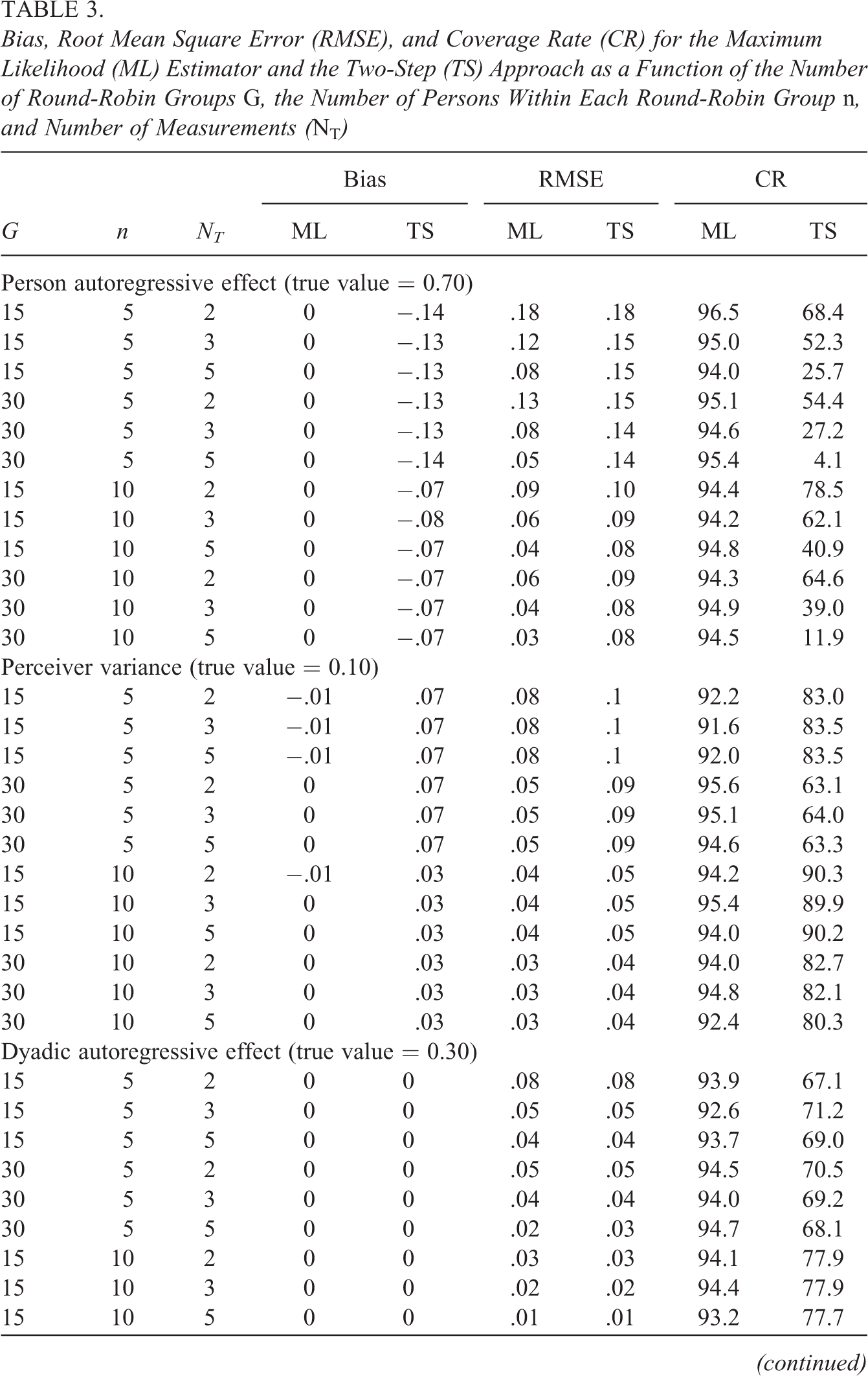
Table 3 contains the results of the simulation for a selection of person-level and dyad-level coefficients. The results for the other coefficients were very similar, and a table containing these coefficients’ results can be found in the accompanying OSF project. The results show that the ML estimator yields unbiased estimates of all model parameters in all simulation conditions. By contrast, the two-step approach yields substantially biased parameter estimates for the person-level coefficients in almost all simulation conditions. However, this bias is smaller in conditions with a larger number of groups (G = 30) and it is negligible for the dyad-level path coefficients (but not the dyad-level variance parameters). The ML estimator, but not the two-step approach, also maintains the nominal coverage in all simulation conditions. The exception are conditions where the number of round-robin groups is small (G = 15) and the number of group members is also small (n = 5). In these conditions, we also see that the two-step approach is sometimes more stable for some of the person-level parameters (i.e., has a smaller relative RMSE). However, the ML approach is always more efficient with a larger number of time points and a larger number of round-robin groups.
Bias, Root Mean Square Error (RMSE), and Coverage Rate (CR) for the Maximum Likelihood (ML) Estimator and the Two-Step (TS) Approach as a Function of the Number of Round-Robin Groups G, the Number of Persons Within Each Round-Robin Group n, and Number of Measurements (NT )
Discussion
In this article, we showed how the SR-SEM, a recently suggested combination of the SRM and the SEM, can be used to estimate different longitudinal data models when longitudinal round-robin data are available. Specifically, we showed how to define the model matrices for an autoregressive SR-SEM and a linear growth SR-SEM. We also described how to interpret the parameters of these matrices in the context of the SRM. The explications of the two example models have hopefully shown that the SR-SEM is a very flexible model that allows researchers to estimate a number of interesting parameters and ultimately to investigate a number of interesting research questions.
The SR-SEM approach has a number of advantages in comparison with earlier approaches that have been suggested for longitudinal SRM data. First, our model can be used to examine longitudinal trajectories in the SRM effects and whether certain person-level or dyad-level covariates can explain between-person or between-dyad differences in these trajectories. Furthermore, due to its one-step nature, our modeling framework is more efficient in comparison to a two-step approach (see also Lüdtke, Robitzsch, & Wagner, 2018). Finally, the ML approach suggested here is a full-information ML approach that allows for missing data in the round-robin variables and the exogenous covariates.
Researchers can specify a number of other models in the SR-SEM that we have not described here. For example, our framework allows for implementing longitudinal state-trait models such as the STARTS model (Kenny & Zautra, 1995, 2001; Lüdtke, Robitzsch, & Wagner, 2018). Furthermore, in our descriptions, we assumed that researchers have assessed a single round-robin variable. However, researchers typically assess multiple round-robin variables. If these variables actually represent different psychological constructs, more complex autoregressive cross-lag panel models can be estimated. For example, when researchers have assessed two round-robin variables, they can examine the cross-lag association between the perceiver effects of the two variables and the target effects of the two variables. In addition to these within-SRM type associations, they can examine the cross-lag association between the perceiver and target effects for the same variable. By contrast, if the variables measure the same construct, one could estimate a kind of second-order linear growth SR-SEM. This model would be interesting not only from an applied but also from a methodological perspective, since it would allow, for example, for testing the invariance of the factor loadings over time. However, we would like to stress that such models for multivariate longitudinal SRM data quickly become very complex, because SRM data are dyadic data. This has the consequence, for example, that there is always a perceiver and a target effect model.
We believe that the SR-SEM framework for longitudinal data is interesting not only for applied but also for methodological researchers. Although the simulation results support the usefulness of the ML approach for estimating the autoregressive SR-SEM parameters, the results of the study are limited, since we do not know whether the same results will emerge when different simulation conditions are examined (e.g., different model population parameters) or when a different model is investigated. Hence, more simulation work is needed to more thoroughly examine the performance of the ML approach. Second, the autoregressive SR-SEM assumes constant time lags between measurements. When this assumption is not met, the parameter estimates may be biased. An interesting task for future research would therefore be to extend continuous time approaches to longitudinal round-robin panel data (Voelkle et al., 2012). Third, another interesting task for future research is to consider nonnormal data. In the present implementation, the SR-SEM assumes that all latent variables are normally distributed. When this assumption is not met, incorrect standard errors may result, so that alternative estimators have to be developed and tested. Fourth, another important question concerns the applicability of model fit indices, which are very often used in the SEM context to evaluate model fit. In the case of SR-SEM, however, the usefulness of fit indices is still unclear because the model works with a complex, nested data structure. Examining this issue in greater detail will be a challenging task for future research. Finally, another important task for future research is to extend the SR-SEM to categorical round-robin data. We believe that—due to the combination with SEM—one can very well rely on work on the categorical SEM for this purpose (e.g., the multitude of weighted least square estimation methods; see Bollen, 1989).
The latter extension is also interesting from a broader modeling perspective because it would allow for comparing the SR-SEM we suggested with social network models, such as temporal extensions of the exponential random graph model (ERGM; Lusher et al., 2013) or the stochastic actor-oriented model (SAOM; Snijders et al., 2010), which are very often used to analyze longitudinal network data. In fact, the SRM and social network models are deeply intertwined, as all round-robin judgments by a group in which each group member rates every other member and each group member is also rated by every member, is a complete social network. The only difference between the two is that the SRM assumes that the (continuous) data are normally distributed, whereas most social network models such as the ERGM or the SAOM are particular cases of a discrete exponential family that are used to analyze binary or more generally categorical data. We believe that an important task for future research is to compare the two approaches with respect to the nature and interpretation of the modeled parameters but also in simulation research with respect to statistical criteria such as bias or coverage.
Conclusion
In this article, we showed how a combination of the SRM with SEM can be used to analyze longitudinal round-robin data. We hoped to demonstrate the flexibility of our approach for the analysis of longitudinal round-robin data. As applied researchers have a growing interest in how interpersonal perceptions, judgments, and behaviors change over time, we believe that our model can offer these researchers an interesting option for analyzing their longitudinal data.
Footnotes
Declaration of Conflicting Interests
The author(s) declared no potential conflicts of interest with respect to the research, authorship, and/or publication of this article.
Funding
The author(s) received no financial support for the research, authorship, and/or publication of this article: This work was supported by Deutsche Forschungsgemeinschaft (NE 1485/7-1, LU 1636/2-2).