
Abstract
Large-scale assessments (LSAs) use Mislevy’s “plausible value” (PV) approach to relate student proficiency to noncognitive variables administered in a background questionnaire. This method requires background variables to be completely observed, a requirement that is seldom fulfilled. In this article, we evaluate and compare the properties of methods used in current practice for dealing with missing data in background variables in educational LSAs, which rely on the missing indicator method (MIM), with other methods based on multiple imputation. In this context, we present a fully conditional specification (FCS) approach that allows for a joint treatment of PVs and missing data. Using theoretical arguments and two simulation studies, we illustrate under what conditions the MIM provides biased or unbiased estimates of population parameters and provide evidence that methods such as FCS can provide an effective alternative to the MIM. We discuss the strengths and weaknesses of the approaches and outline potential consequences for operational practice in educational LSAs. An illustration is provided using data from the PISA 2015 study.
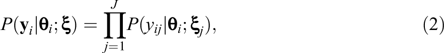
One of the main goals of educational large-scale assessments (LSAs) such as the Programme for International Student Assessment (PISA) and the Trends in International Mathematics and Science Study (TIMSS) is to provide information about student proficiency and the relations between student proficiency and other cognitive and noncognitive variables such as students’ socioeconomic status, self-concept, attitudes, or interests (Singer & Braun, 2018). To this end, LSAs employ scaling procedures by which proficiency scores are estimated for each student on the basis of (a) their performance on an achievement test and (b) the information they provide in a background questionnaire. Combining these two sources of information, the scaling procedure is often used to generate a set of “plausible values” (PVs) for the proficiency of each student (Mislevy, 1991). This method follows Rubin’s (1987) multiple imputation (MI) approach by regarding the latent proficiency scores as missing data and allows for unbiased estimates of population parameters (Mislevy, 1991; Mislevy, Johnson, & Muraki, 1992; for other approaches to estimating population parameters, see also Culpepper & Park, 2017; Rijmen et al., 2014; von Davier & Sinharay, 2007, 2010).
An important requirement of these scaling procedures is that the background variables are completely observed. However, missing data are common in LSAs. They occur, for example, because students fail to answer some of the items in the background questionnaire or because some studies use a rotated questionnaire (or planned missing data) design (Graham et al., 2006; Rhemtulla & Hancock, 2016). For example, socioeconomic status is often missing for a substantial number of participants, thereby making it difficult to derive statements about the relation between students’ socioeconomic background and educational attainment. This difficulty raises the question of how missing data in background variables should be treated in educational LSAs.
The treatment of missing data in LSAs is further complicated by the fact that the data are prepared and used by two different parties sometimes called the “imputer,” whose task is to generate the PVs, and the secondary “analyst” who uses the data to answer a substantive research question (Meng, 1994; see also Shin, 2013). For the imputer, an ideal statistical procedure would allow for the generation of PVs while simultaneously treating the missing data in background variables (e.g., using MI; see also Blackwell et al., 2017a, 2017b). No such procedure is currently used in educational LSAs. Instead, LSAs rely on the missing indicator method (MIM; Cohen & Cohen, 1975) whose application has been discouraged in the statistical literature (e.g., Jones, 1996; Schafer & Graham, 2002). For the analyst, this method creates additional challenges because, although it provides PVs, it does not provide imputations for missing data and requires that these be treated by other means.
Several articles have investigated the treatment of missing data in background variables. von Davier (2013) provided a discussion of the challenges associated with rotated questionnaires in LSAs. Adams et al. (2013) investigated the effects of rotated questionnaires on the estimates of population parameters and concluded that these designs allow for accurate estimates of the marginal properties of student proficiency (e.g., population means). However, Rutkowski (2011) and Rutkowski and Zhou (2015) found that the current treatment of missing data in LSAs can lead to biased parameter estimates in subpopulations (e.g., means and mean differences) when missing data occur in a systematic manner. Kaplan and Su (2016, 2018) showed that different rotated questionnaire designs can differ greatly in how well they recover variables’ marginal properties and the relations between them. For the treatment of missing data, Assmann et al. (2015) proposed a Bayesian estimation procedure for estimating the scaling model with missing background data, and Weirich et al. (2014) evaluated procedures based on two-stage (or nested) MI (see also Harel, 2007; Rubin, 2003). Finally, Wetzel et al. (2015) considered alternatives to the current practice based on latent class models.
In writing this article, we had three goals. First, we aimed to evaluate the procedures currently used for handling missing data in background variables in educational LSAs (i.e., those based on the MIM) in an attempt to clarify the conditions under which they can cause problems. Second, we aimed to implement and evaluate a strategy that allows for a joint modeling of PVs for the proficiency scores and imputations of missing data in background variables. Finally, we attempted to contrast the strengths and weaknesses of these approaches and provide recommendations for the operational practices applied in educational LSAs.
The article is organized as follows. In the first section, we review the statistical procedures used in the scaling of proficiency data and the generation of PVs in educational LSAs. In the second and third sections, we extend our discussion to the case with missing data in background variables, reviewing (a) the current practices applied in educational LSAs (based on the MIM) and (b) the joint modeling of measurement error and missing data. We then present the results of two simulation studies in which we evaluated the performance of these methods in two scenarios with different measurement models and statistical complexity. Finally, we illustrate their application with data from the PISA 2015 study (Organization for Economic Cooperation and Development [OECD], 2017). We close with a discussion of our findings and recommendations for practice.
Statistical Models in LSAs
The statistical procedures used in educational LSAs are applied to represent the relations between students’ responses on the achievement test, their latent (i.e., unobserved) proficiency on these tests, and their responses on the background questionnaire. Let

where
Scaling Model
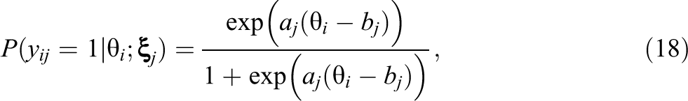
In educational LSAs, the students’ responses to the items on the achievement test are modeled with item response theory (IRT), which describes item responses as a function of both person ability and item characteristics. In general, IRT models express the probability of observing a response pattern
where
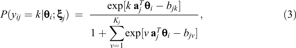
where the item parameters
Population Model and PVs
The generation of PVs follows Rubin (1987) by regarding the latent proficiency scores as missing data, for which imputations can be generated by drawing repeatedly from the posterior predictive distribution of the proficiency

where the first term denotes the scaling model with item parameters

where
This procedure for generating PVs can be used directly when the background variables are completely observed. In practice, however, the background variables often contain missing data and require treatment before the PVs can be generated (Adams et al., 2013; Wetzel et al., 2015). In the following, we describe the method currently used to deal with missing data in the background questionnaire in LSAs and consider its statistical properties.
Missing Data in the Background Questionnaire
In educational LSAs, the background variables are seldom complete. Suppose that some elements of
The current method for dealing with missing data in the background variables in LSAs relies on including the indicator variables
Missing Indicator Method
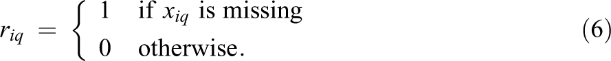
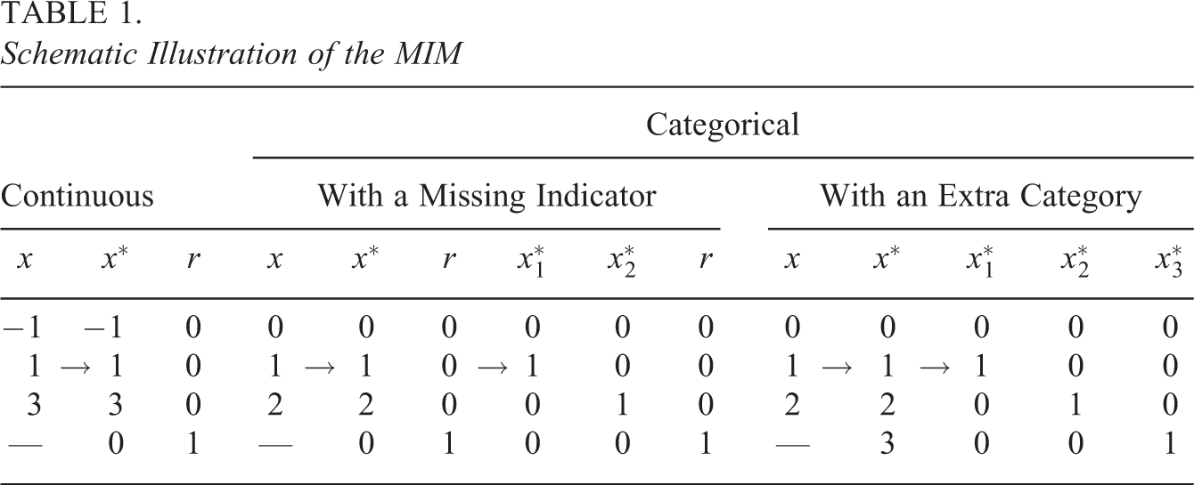
The general idea behind the MIM is to recode the incomplete background questionnaire data by replacing missing data with predefined values and by including additional indicator variables that represent differences between cases with missing and observed data, respectively (Adams et al., 2013). The MIM can be applied to both continuous and categorical data, which is illustrated in Table 1. For any background variable with missing data xq , an indicator variable rq is created such that
In addition, the background variables are recoded to render them temporarily complete. A continuous background variable xq
, possibly centered at its mean or median, is recoded into a new variable

This is illustrated in Table 1. For categorical data, the same principle is used but combined with dummy or effect coding. For example, when using dummy codes to represent a categorical variable xq
with Lq
categories and values
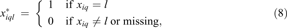
where the remaining category acts as a reference category. This strategy is sometimes described as treating missing responses as an “extra category” because the missing indicator rq acts as an additional dummy variable in the coding scheme. In other words, treating missing responses as an extra category is equivalent with coding missing responses as zero and adding a missing indicator to the coding scheme. This is illustrated in Table 1 for a single variable with three categories.
Schematic Illustration of the MIM
The recoded variables

Because the variables
Despite its convenience, the MIM has been criticized because it can distort parameter estimates (Jones, 1996). The same may be true in LSAs when PVs are generated under the MIM (see also Rutkowski, 2011). Furthermore, because the MIM provides only a temporary solution to missing data in background variables, secondary analysts must take additional steps to treat them, for example, by removing cases with incomplete data (e.g., listwise deletion) or by using MI (see also Schafer & Graham, 2002). 3 It is largely an open question whether using the MIM, by itself or in combination with these methods for handling missing data, can provide unbiased estimates of population parameters in LSAs. In the following, we consider this question in more detail.
Estimators Under the MIM
Depending on the method used to treat missing data after generating the PVs via the MIM, it is possible to obtain different estimators for population parameters. In the following, we consider three such methods: pairwise estimation of variances and covariances (MIM-PE), listwise deletion (MIM-LD), and nested MI of the incomplete data (MIM-MI). The three methods provide different estimators for the population parameters that differ in how they make use of the data. Specifically, MIM-PE estimates variances and covariances on the basis of the (pairwise) available data, and other parameters such as correlation or regression coefficients are then estimated on the basis of the variance-covariance matrix. MIM-LD estimates variances and covariances in the same way, but other parameters such as correlation and regression coefficients are obtained on the basis of only the subset of the data in which all of the required variables are complete. Finally, MIM-MI generates replacements for missing data in background variables on the basis of the PVs generated under the MIM and the observed data, and the population parameters of interest are then estimated on the basis of the imputed data.
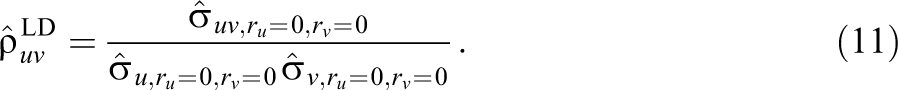
To illustrate the difference between the estimators, consider a hypothetical scenario with two variables u and v, both of which contain missing data. In this case, there are two missing data indicators ru and rv . Suppose the parameter of interest is the correlation between u and v. Using MIM-PE, the correlation is estimated by first estimating the variances and covariances of the variables using the (pairwise) available data, that is,

where the subscripts refer to the subsets of the data in which u and v are observed (
Although the two estimators use the same information about the covariance between the variables, they make different use of the information that is available about the variances. The same principle applies more generally to all parameters whose sufficient statistics include the variance-covariance matrix of the variables. For example, suppose that

The sufficient statistics for the regression coefficients (ignoring the intercept) are the variances and covariances among the variables, and the coefficients can be estimated as

In MIM-PE, the variances and covariances are estimated using the (pairwise) available data, that is, every element in the variance-covariance matrix is estimated separately using the data available for the respective (pair of) variables. In MIM-LD, all values in the variance-covariance matrix are estimated at once using the subset of the data in which all variables are observed. Finally, in MIM-MI, the variances and covariances are estimated using the imputed data. In the following, we discuss the statistical properties of the different estimators under the MIM in more detail.
Statistical Properties of the MIM
To better understand the statistical properties of the MIM, we derived the asymptotic bias in the parameter estimates under the MIM in a “minimal” setting with one latent variable
Expected Values for the Estimated Variances and Covariances Under the MIM Organized by the Pattern of Missing Data and the Method Used to Treat Missing Data Under MCAR
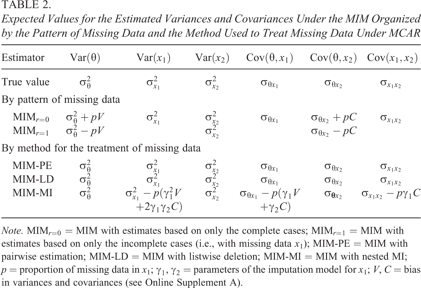
Note. MIM
Pairwise estimation
Our investigation showed that, under MIM-PE, the variances and covariances can be estimated without bias under MCAR. Consequently, this would also allow for an unbiased estimation of other parameters such as correlation and regression coefficients by employing a two-step procedure in which the variances and covariances of the variables are estimated in a pairwise fashion, and regression coefficients are then calculated on the basis of the variance-covariance matrix. This is an important finding because it shows that unbiased estimates of many key parameters can be obtained under the MIM at least when the data are MCAR.
Listwise deletion
Under MIM-LD, the variances and covariances are estimated without bias, as with MIM-PE. However, the estimates of correlation and regression coefficients can be biased even when the data are MCAR. This is because variances and covariances can be biased in the subsets of the data that pertain to complete and incomplete cases, respectively (MIM

where
Nested MI
Under MIM-MI, some but not all variances and covariances can be estimated without bias (see Table 2). Specifically, because the estimates of the variances and covariances in the subsets of the data pertaining to complete and incomplete cases (MIM
In summary, our investigation suggested that, although unbiased estimates can be obtained with MIM-PE, naive use of MIM-LD or even MIM-MI can lead to distorted parameter estimates even if the data are MCAR. Nonetheless, these results should be interpreted with care due to the restrictive nature of the assumptions made in their derivation. In the following section, we present an alternative to the MIM based on a joint treatment of PVs and missing data in the background questionnaire. Then, we present the results of two simulation studies that we conducted to evaluate these procedures in more general and realistic scenarios.
Joint Treatment of PVs and Missing Data
If there are missing data in the background variables, the joint distribution of

where
In order to draw inferences on the basis of only the observed data, the missing data can be “integrated out” of the function used to fit the model of interest (e.g., the likelihood function or the posterior distribution; see Little & Rubin, 2002). The following posterior distribution for the missing data and the latent proficiency scores can then be used to draw PVs for

Finally, inferences about population parameters can be drawn by averaging over the PVs for
Sampling From the Joint Distribution
There are several computational approaches to sampling from the joint distribution of
FCS algorithm
The general idea of FCS is to approximate draws from the joint posterior distribution of
For every latent proficiency
Draw
Impute
For every background variable
Draw
Impute
Notice that the FCS algorithm divides the sampling of the multidimensional proficiency
Study 1
In the first study, we focused on a minimal setting, which included a 2PL IRT measurement model and two continuous background variables, one of which contained missing data.
Data Generation
The data were simulated from a multivariate normal distribution with three variables

where
where the item parameters
Missing data
Missing data were induced in x
1 on the basis of a latent response propensity

where
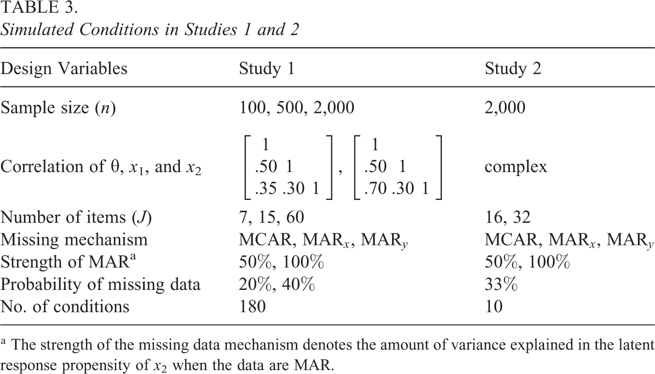
The simulated conditions are summarized in Table 3 and were chosen so that they reflected typical conditions in LSAs or were of theoretical interest. Specifically, we varied the sample size (
Simulated Conditions in Studies 1 and 2
Scaling and imputation procedures
In the scaling model for
Scaling and Imputation Procedures in Study 1
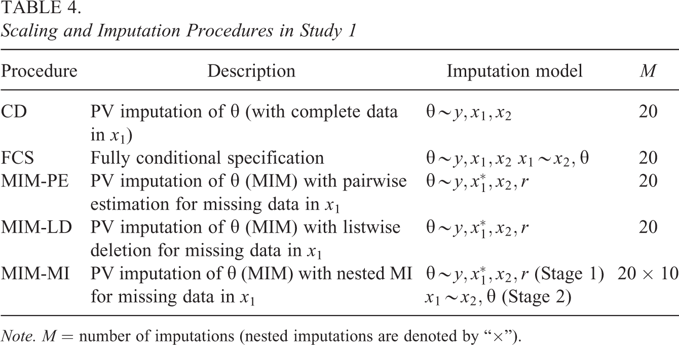
Note. M = number of imputations (nested imputations are denoted by “
Parameters of interest and pooling
The parameters of interest included the means, variances, and covariances for all variables as well as their correlations and the regression coefficients for the regression of
Results
Because the simulation yielded many results, we focus on only the main findings here.
Bias
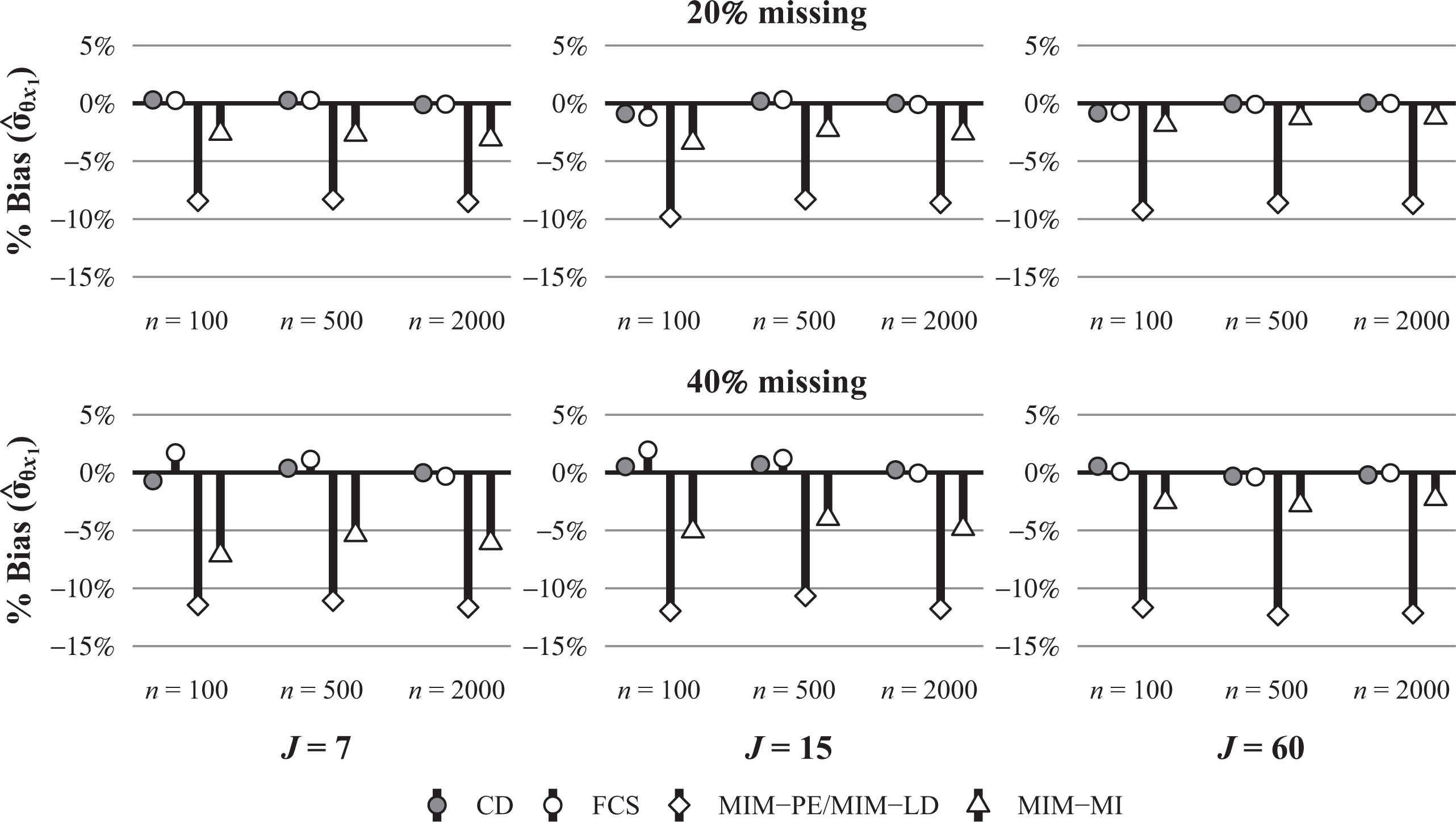
Figure 1 shows the estimated bias for the mean and variance of
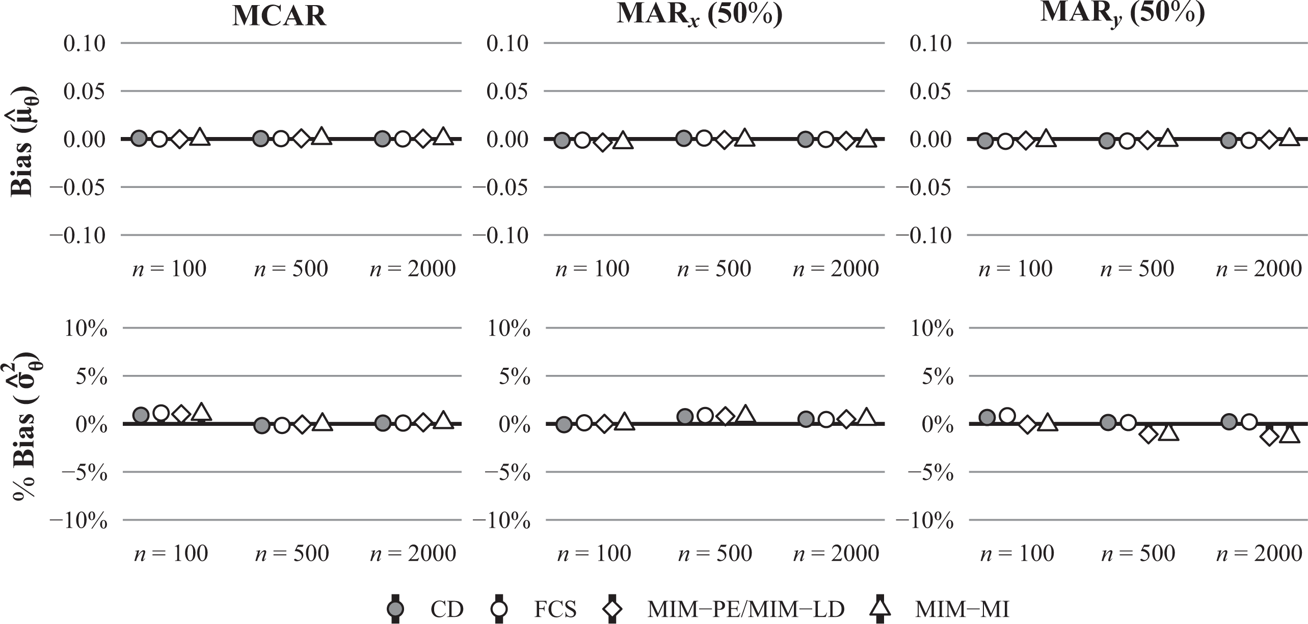
Bias (raw and in %) for the estimated mean and variance of θ in conditions with a moderate number of items (J = 15), a strong correlation between θ and x2 (
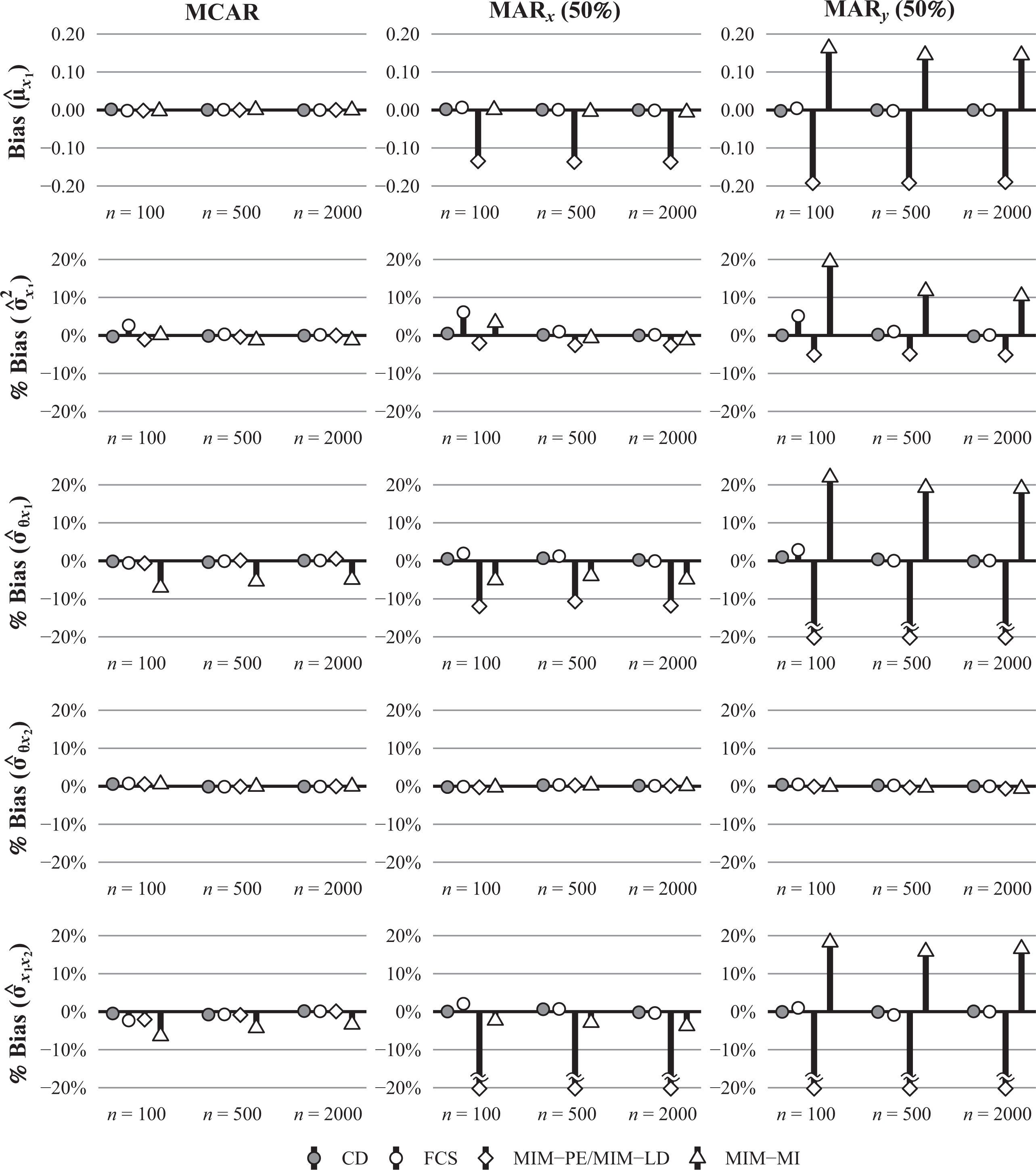
Bias (raw and in %) for the estimated the mean and variance of x1 and the covariances between θ, x1, and x2 in conditions with a moderate number of items (J = 15), a strong correlation between θ and x2 (
Bias (in %) for the estimated covariance between
In addition to the means, variances, and covariances, we also investigated the bias in the estimates of the correlations between variables and the regression coefficients in the multiple regression of
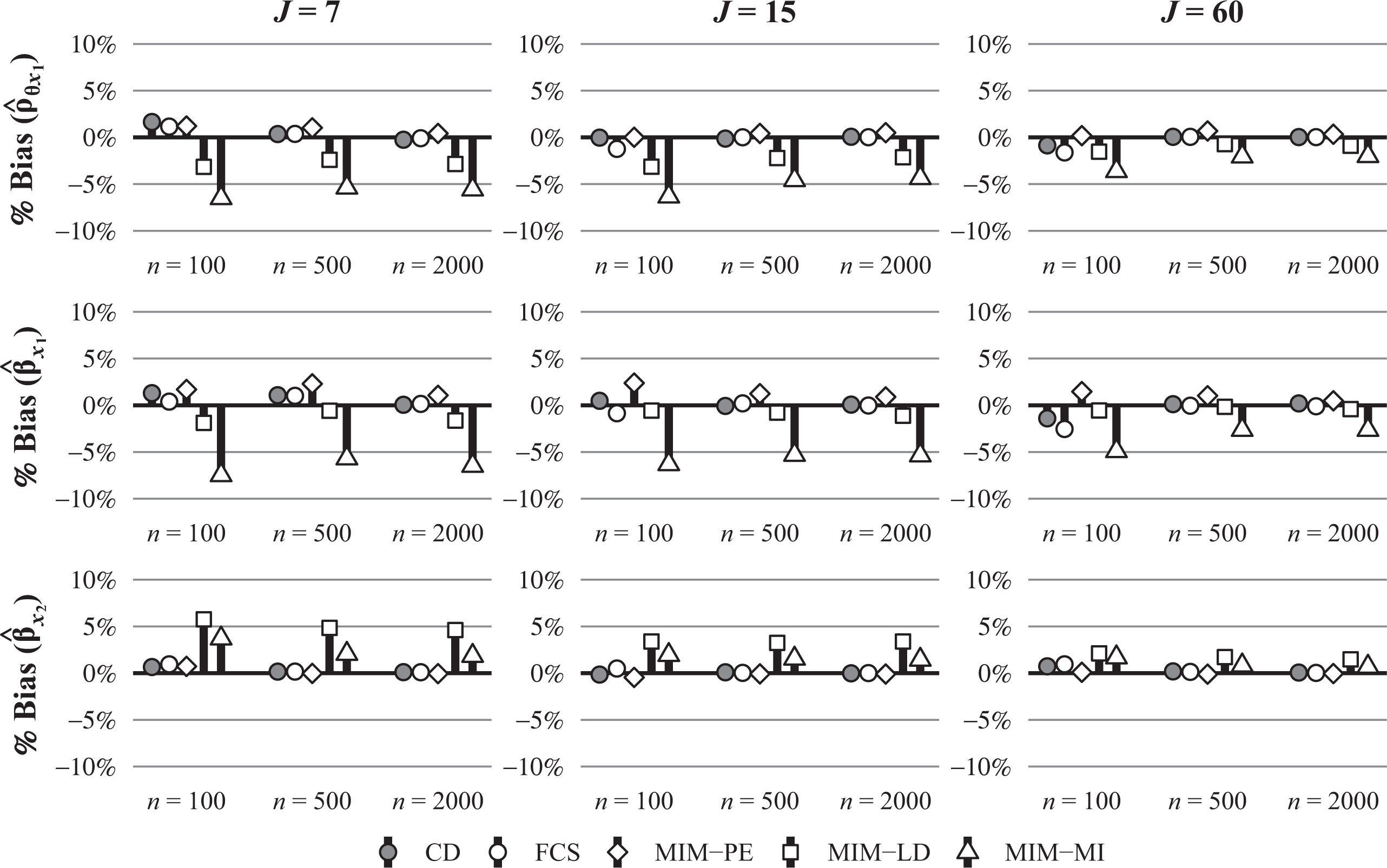
Bias (in %) for the estimated regression coefficients in the regression of θ on x1 and x2 in conditions with a strong correlation between θ and x2 (
RMSE
The RMSE followed a pattern similar to the bias and was usually lower under FCS than under MIM-LD, MIM-PE, and MIM-MI. However, despite the fact that the parameter estimates were sometimes biased under MIM-LD and MIM-MI, they were sometimes more accurate (i.e., had a lower RMSE) than under FCS. This was the case primarily in small samples (
Coverage
The results for the coverage rates of the 95% confidence intervals are shown in Table 5 for the estimated correlation between
Coverage of the 95% Confidence Interval for the Correlation of θ and x1 With a Strong Correlation of
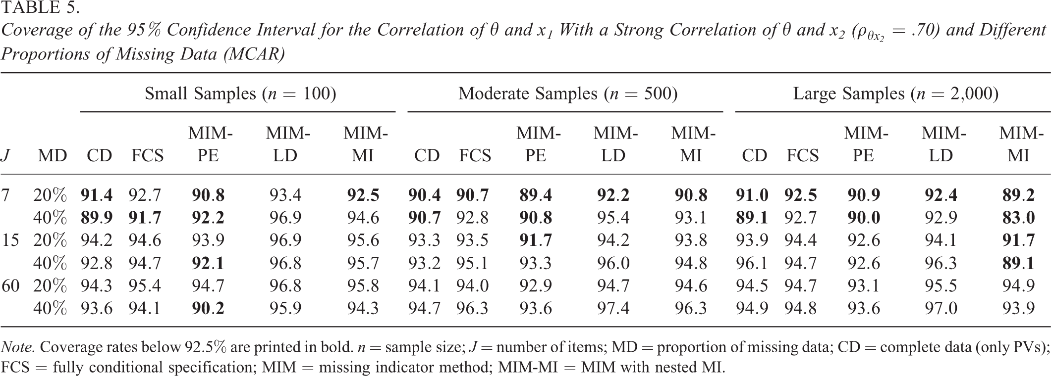
Note. Coverage rates below 92.5% are printed in bold. n = sample size; J = number of items; MD = proportion of missing data; CD = complete data (only PVs); FCS = fully conditional specification; MIM = missing indicator method; MIM-MI = MIM with nested MI.
Summary
The results of Study 1 illustrate several important points. First, the application of the MIM allows for unbiased estimates of the mean and variance of
Study 2
In the second study, we extended the simulation setting to be more similar to conditions commonly found in LSAs. Because the simulation design is much more complex than in the first study, we only provide a brief overview here. For a complete description, we refer to Online Supplement D.
Data Generation, Procedures, and Parameters of Interest
The second simulation featured an extended design with a latent proficiency variable
The scaling and imputation procedures were the same as in the previous study (i.e., CD, FCS, MIM-PE, MIM-LD, and MIM-MI). In accordance with the operational practices applied in LSAs, we converted the background variables into contrast codes and used principal components analysis (PCA) to extract 100 principal components, which were then used as conditioning variables in the latent regression model. Under the MIM, the effect coding also included additional codes to indicate missing responses for each variable (i.e., treating missing responses as an “extra category”). For FCS and MIM-MI, we imputed missing data in the background variables using predictive mean matching (PMM). 6 For CD, FCS, and the MIM, we generated 10 PVs, and for MIM-MI, we generated five imputations for every PV, resulting in a total of 50 imputations.
The parameters of interest were the means, variances, and covariances among the variables as well as the correlations between the variables and the regression coefficients for the multiple regression of
Results
The estimated bias in the means, variances, and covariances of the variables is summarized in Table 6 for each type of parameter that pertains to background variables in different blocks of the background questionnaire (
Summary of the Estimated Bias in Estimated Means, Variances, and Covariances by Block (
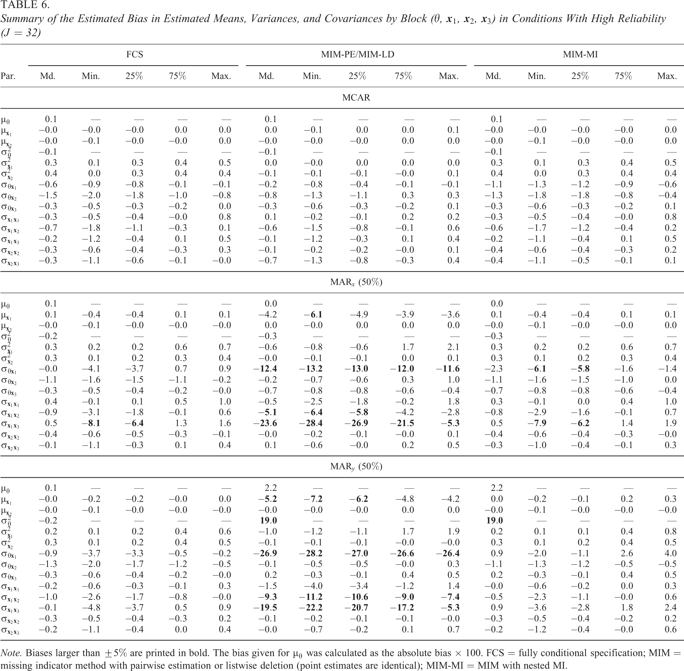
Note. Biases larger than
Similar to the first study, we also investigated bias in the correlation and regression coefficients. This is illustrated in Figure 5 for the correlations of
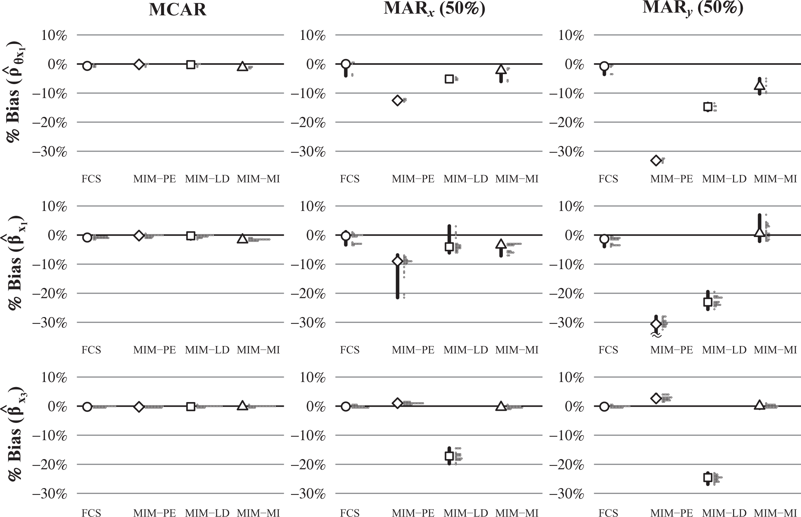
Bias (in %) for the estimated correlation coefficients of θ with
Summary
The second simulation study provided some important insights about the statistical properties of the methods we considered. First, although the theoretical properties of the methods based on the MIM (MIM-PE, MIM-LD, and MIM-MI) suggested that a naive use of MIM-LD and MIM-MI may lead to biased parameter estimates even when the data are MCAR, this may not necessarily be a reason for concern in the context of educational LSAs, where the large number of background variables may compensate for the effects of missing data under the MIM. This is an encouraging finding because it illustrates that the MIM allows for approximately unbiased parameter estimates at least under MCAR. However, under MAR
Example Analysis: PISA 2015
To illustrate the procedures considered in this article, we used data from the German subsample (N = 6,504) of PISA 2015 (OECD, 2017). The data included the 184 cognitive items from the science domain and 214 variables from the students’ background questionnaire. Missing data occurred in all cognitive items (range: 77.8%–92.6%) and almost all of the background variables (range: 10.9%–54.0%). The procedures were implemented in a manner that was similar to the operational practices used in PISA 2015. In the interest of space, we only provide a brief description of the procedures here and provide a full description along with the computer code in Online Supplement E. We generated the PVs using the item parameters and contrast coding scheme used in PISA 2015 (OECD, 2017) and the R package TAM (Robitzsch et al., 2018). This entailed the use of dummy codes to indicate missing responses for all background variables, which were then subjected to PCA in order to obtain components that we used as conditioning variables in the latent regression model. To impute the missing data, we used a FCS approach based on the R package mice (van Buuren & Groothuis-Oudshoorn, 2011), where categorical and ordinal variables were imputed with polytomous regression models and PMM, respectively (see also Kaplan & Su, 2016, 2018). The imputation methods for the background variables also used the contrast-coded background data but relied on partial least squares (PLS) to reduce the dimensionality of the data. All steps in the procedure included the final student weights.
For the analysis of the data, we obtained WLEs for each of the 25 noncognitive scales from the background questionnaire using the item parameters used in PISA 2015. The parameters of interest were the regression coefficients in the regressions of science proficiency on any two of the noncognitive scales from the background questionnaire. This resulted in 600 regression coefficients (not counting the intercept) obtained from 300 regression analyses. For MIM-PE and MIM-LD, the WLEs were calculated only for students who responded to at least three items of that scale and set to missing otherwise (see also OECD, 2017). The results are summarized in Figure 6, which provides a direct comparison of the parameter estimates obtained from different procedures. Overall, the regression coefficients obtained from the three procedures were similar with differences primarily occurring between MIM-PE and MIM-LD on the one hand and FCS and MIM-MI on the other hand, such that the estimates under MIM-PE and MIM-LD tend to be somewhat closer to zero. This difference is visible both in the correlation and the mean absolute difference between the procedures as well as in the slight “tilt” that is present in some of the panels of the figure. However, in summary, these results are in line with the results of the simulation studies and illustrate that, whereas differences between the procedures can sometimes be observed, the differences were relatively small in most cases, especially when there were many background variables available and the (conditional) reliability of the test was high.
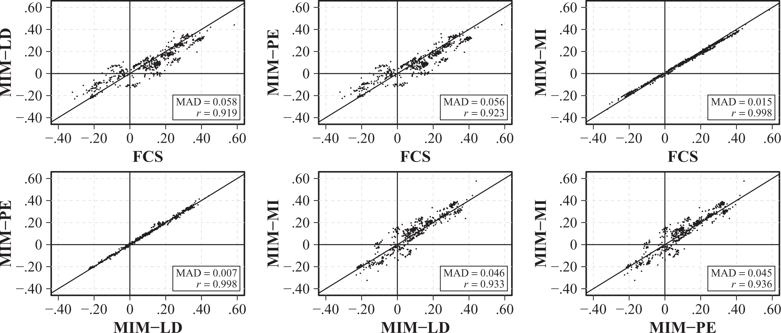
Comparison of the estimated standardized regression coefficients from the regressions of the PVs on any two background variables in the example analysis obtained from different procedures. MAD = mean absolute difference; r = correlation; FCS = fully conditional specification; MIM-PE = missing indicator method with pairwise estimation; MIM-LD = MIM with listwise deletion; MIM-MI = MIM with nested MI.
Discussion
In this study, we investigated different procedures for the treatment of missing data in background variables in educational LSAs. This included the joint treatment of proficiency scores and missing data (i.e., FCS) as well as the procedures currently used in operational practice (i.e., the MIM), combined with different methods for the treatment of missing data (MIM-PE, MIM-LD, MIM-MI). From a theoretical perspective, our investigation revealed that the MIM can provide unbiased results when the data are MCAR. This included estimates of means, variances, and covariances, but it required the use of a pairwise estimation strategy (MIM-PE) for more complex parameters such as correlation and regression coefficients, whereas its use with listwise deletion (MIM-LD) or MI (MIM-MI) sometimes led to biased parameter estimates even under MCAR. In two simulation studies, we investigated these properties across a wider range of conditions. In all conditions, we found that the FCS procedure provided unbiased estimates with good inferential properties. By contrast, the MIM provided unbiased estimates only when the data were MCAR but not when they were MAR, in which case the bias tended to be lowest when the MIM was combined with MI (MIM-MI). However, in conditions with a larger number of background variables, which are the most similar to conditions encountered in LSAs, the differences between the procedures were much less pronounced, indicating that some of the negative properties of the MIM can be compensated for with the large amount of information available in LSAs. In particular, we found that the MIM when combined with MI often provided results similar to FCS in these conditions for all except a few of the parameters of interest.
Overall, these results are encouraging because they (a) illustrate a number of positive theoretical properties of the MIM that hold when the data are MCAR (i.e., with rotated questionnaires; see also Adams et al., 2013) and (b) provide additional support for the recommendations already in place regarding the analyses of incomplete background data with rotated questionnaires in educational LSAs (e.g., for MIM-PE and MIM-MI; see also OECD, 2014). However, the results also highlight some possible weaknesses of the MIM, namely, that (a) parameter estimates might not be completely unbiased when the data are MAR even when MI is used and (b) some parameter estimates may be biased even when the data are MCAR when obtained with listwise deletion, which is the default setting for many analyses in statistical software.
Based on our findings, it may be worth considering the joint treatment of proficiency scores and missing data as an alternative to the operational practices applied in educational LSAs. However, this idea can be met with scrutiny: Not only does a joint treatment complicate the generation of PVs, but it also blurs the line between the imputer and the (secondary) analyst by placing the burden of specifying an imputation model for the missing background data on the imputer. This requires the imputer to anticipate potential analyses, so that the imputation model will “fit” the intended analyses (Meng, 1994). However, this problem is not unique to the treatment of missing data and applies to the generation of the PVs in the same way. In principle, it may be worth considering whether the data for secondary analyses could be released in two versions: one containing PVs and imputations for missing background data and one containing only the PVs but with the imputations for missing data deleted. In this context, two-stage or nested MI (Rubin, 2003)—in which the PVs for the latent proficiency variables and the imputations for the missing background data are generated in two separate stages—may be considered as an alternative. The little research that has evaluated these approaches seems to imply that they enjoy qualities similar to the joint imputation of PVs and missing data (Weirich et al., 2014; see also Kaplan & Su, 2018).
The implementation of the FCS approach considered here is only one of several ways to adopt a joint imputation of PVs and missing data. First, the FCS approach is not restricted to the use of univariate models to generate PVs, and multivariate models can be used instead to maintain the multidimensional scaling procedures employed in educational LSAs (see von Davier & Sinharay, 2013). To our knowledge, such an approach is currently not implemented in statistical software. Second, instead of using an FCS approach, the joint distribution of the variables can sometimes be modeled directly (Blackwell et al., 2017a, 2017b; King et al., 2001; see also Cole et al., 2006). Third, the FCS approach presented here uses parametric models for the treatment of missing data. By contrast, nonparametric methods (e.g., Assmann et al., 2015; Si & Reiter, 2013) or procedures based on latent class models may allow for an even more flexible representation of the relations (and possible interactions) between the variables (Vermunt et al., 2008; Vidotto et al., 2018; Wetzel et al., 2015; Xu & von Davier, 2019; see also von Davier, 2013). Finally, the imputation of PVs need not be restricted to the achievement test data but can also be applied to the noncognitive constructs in the background questionnaire (e.g., interest and attitude scales). In other words, missing data need not be imputed on the item level but may be combined with intermittent steps to generate PVs for these scales (see also Gottschall et al., 2012).
This study comes with multiple limitations and points to consider. First, educational LSAs often feature hundreds of variables that require the dimensionality of the data set to be reduced before the scaling model can be applied. For this purpose, PCAs or PLS can be used (Oranje et al., 2009; Oranje & Ye, 2013). This was illustrated in our analysis of the PISA 2015 data, in which we used PLS to reduce the dimensionality of the imputation models for the background variables. Second, the data in educational LSAs often have a multilevel structure that results from students being clustered in schools. This structure needs to be taken into account in the scaling of the proficiency data (Adams et al., 1997; Adams & Wu, 2007; Li et al., 2009), the imputation of missing background data (Enders et al., 2016; Lüdtke et al., 2017), and secondary analyses (Monseur & Adams, 2009). By contrast, if the multilevel structure is represented with fixed effects, such as in PISA, then the methods considered in this article can be applied directly by including an additional set of indicator variables to represent school membership in the imputation models for missing data and the PVs (see the example with the PISA 2015 data).
Further research is needed to fully understand the proper treatment of missing data in background variables in educational LSAs. This includes the comparison of the available methods in a wider range of settings, for example, when the data are MNAR (see also Ibrahim et al., 2005; Moustaki & Knott, 2000; O’Muircheartaigh & Moustaki, 1999). The same is true for applications with rotated questionnaire designs that are gaining popularity in educational LSAs. The procedures studied in this article can be applied to missing data that stem from rotated questionnaires, but their performance under different forms of rotation is an important topic that has yet to receive more attention (see also Kaplan & Su, 2016, 2018). Finally, future research should take into account the relationship between the imputer and the (secondary) analyst (Meng, 1994). This is particularly important because the data from educational LSAs are often used for a variety of purposes, comprising an immense number of potential analyses (e.g., models with nonlinear effects, multilevel models; see also Li et al., 2009; Schofield, 2015; Schofield et al., 2015).
Supplemental Material
Supplemental Material, Supplement_MIM_20200826 - On the Treatment of Missing Data in Background Questionnaires in Educational Large-Scale Assessments: An Evaluation of Different Procedures
Supplemental Material, Supplement_MIM_20200826 for On the Treatment of Missing Data in Background Questionnaires in Educational Large-Scale Assessments: An Evaluation of Different Procedures by Simon Grund, Oliver Lüdtke and Alexander Robitzsch in Journal of Educational and Behavioral Statistics
Footnotes
Declaration of Conflicting Interests
The author(s) declared no potential conflicts of interest with respect to the research, authorship, and/or publication of this article.
Funding
The author(s) received no financial support for the research, authorship, and/or publication of this article.
Notes
References
Supplementary Material
Please find the following supplemental material available below.
For Open Access articles published under a Creative Commons License, all supplemental material carries the same license as the article it is associated with.
For non-Open Access articles published, all supplemental material carries a non-exclusive license, and permission requests for re-use of supplemental material or any part of supplemental material shall be sent directly to the copyright owner as specified in the copyright notice associated with the article.