Sage Journals: Discover world-class research

Abstract

The rapid serial visual presentation (RSVP) paradigm has garnered considerable attention in brain–computer interface (BCI) systems. Studies have focused on using cross-subject electroencephalogram data to train cross-subject RSVP detection models. In this study, we performed a comparative analysis of the top 5 deep learning algorithms used by various teams in the event-related potential competition of the BCI Controlled Robot Contest in World Robot Contest 2022. We evaluated these algorithms on the final data set and compared their performance in cross-subject RSVP detection. The results revealed that deep learning models can achieve excellent results with appropriate training methods when applied to cross-subject detection tasks. We discussed the limitations of existing deep learning algorithms in cross-subject RSVP detection and highlighted potential research directions.

Keywords

rapid serial visual presentation brain–computer interface cross-subject deep learning detection

1 Introduction

Brain–computer interface (BCI) systems are a promising technology of communication and control for individuals with disabilities. BCI systems allow people with disabilities to interact with their environment through their brain signals [1, 2]. P300 is a widely used BCI paradigm that is based on the event-related potential (ERP) component that occurs in response to the target stimuli [3]. The P300 component has distinctive temporal and spatial properties, with a latency of approximately 300 ms and a central-parietal distribution [4]. The P300 speller proposed by Farwell and Donchin has been studied extensively [5], and various algorithms, such as denoising autoencoder [6], BN3 [7], ST-CapsNet [8], MsCNN [9], have been proposed. Rapid serial visual presentation (RSVP) is another popular BCI paradigm in which stimuli are presented in a rapid sequence. In RSVP, target stimuli are presented among distractors, and the BCI detects the target stimuli [10, 11]. The classification of single-trial RSVP EEG signals is essential for developing an effective and reliable BCI system.

Conventional algorithms for single-trial RSVP EEG classification include linear discriminant analysis (LDA), Fisher discriminant analysis (FDA), and spatial weighted FLD-PCA (SWFP). Although LDA is a simple and effective algorithm [12], it has several limitations because of its linear assumption of data. Fisher discriminant analysis is another algorithm in which the Fisher criterion is used to determine the optimal linear combinations of EEG features for classification [13]. By contrast, SWFP is designed for single-trial RSVP detection and exhibits better performance than hierarchical discriminant component analysis (HDCA) [14] and hierarchical discriminant principal component analysis algorithm (HDCPA) [15]. SWFP is a complex algorithm in which both spatial and temporal information is considered. However, SWFP requires the manual selection of the best feature set. Therefore, the model can be time-consuming and subjective [15].

Deep learning algorithms are increasingly being used for single-trial RSVP EEG classification. For example, EEGNet, is a robust deep learning algorithm with a compact convolutional neural network (CNN) that achieves high accuracy and fast classification of EEG signals [16]. In DeepConvNet, a deeper CNN architecture with additional max pooling and dense layers are used to improve classifier robustness [17]. However, DeepConvNet is computationally more expensive than EEGNet is. To improve ERP detection performance, Santamaria-Vazquez et al. proposed EEG-Inception to integrate the inception module into ERP detection. Thus, a multiscale temporal convolution kernel was used to accurately extract the temporal features of ERP [18]. Studies have supported the claim that using multiscale convolution kernels can enhance model performance. For example, Wang et al, who won the P300-based speller BCI competition at the World Robot Contest (WRC) 2019, proposed multiscale CNN to enhance the performance of P300 detection [19]. In this model, three temporal kernels at different scales were applied on its temporal convolution layer to obtain discriminative time features.

Conventional machine learning can achieve excellent results for RSVP classification. Wu, who was awarded in the ERP final competition of the WRC 2021, proposed a novel method for improving the classification performance of RSVP across subjects [20]. In this method, first, the ERP data is aligned across subjects using Euclidean alignment after preprocessing. This step is crucial because ERP data can vary considerably between subjects. When the data are aligned, Wu used xDAWN [21] and tangent space mapping to extract ERP features. These features are then used to train a logistic regression classifier. The results revealed that Wu’s method considerably improved the classification performance of RSVP across subjects [22]. Furthermore, combining conventional spatial filtering estimation with deep learning methods improved performance. For example, in the improved EEGNet proposed by Zhang et al., the EEG signal was first spatially filtered with xDAWN and subsequently inputted into EEGNet for processing [23]. However, underfitting occurs when the amount of data are large when conventional machine learning algorithms are used. For the ERP competition at WRC 2022, organizers prepared training data from 24 people with approximately 360,000 samples. Deep learning models should be more appropriate for these samples than conventional machine learning methods because methods exhibit superior data fitting capability. The top 5 winning teams in the final competition adopted deep learning methods. In this study, we proposed the algorithms of the top five winning teams in the ERP finals and compared the results of these teams.

2 Methods

2.1 Experimental paradigm

In this RSVP experiment, three types of images, including two types of targets (people and cars) and one type of background (unoccupied street scenes without cars), were used. All images were captured from street scenarios, and the image sequences were presented to the subjects by using the RSVP paradigm (Fig. 1).

Fig. 1

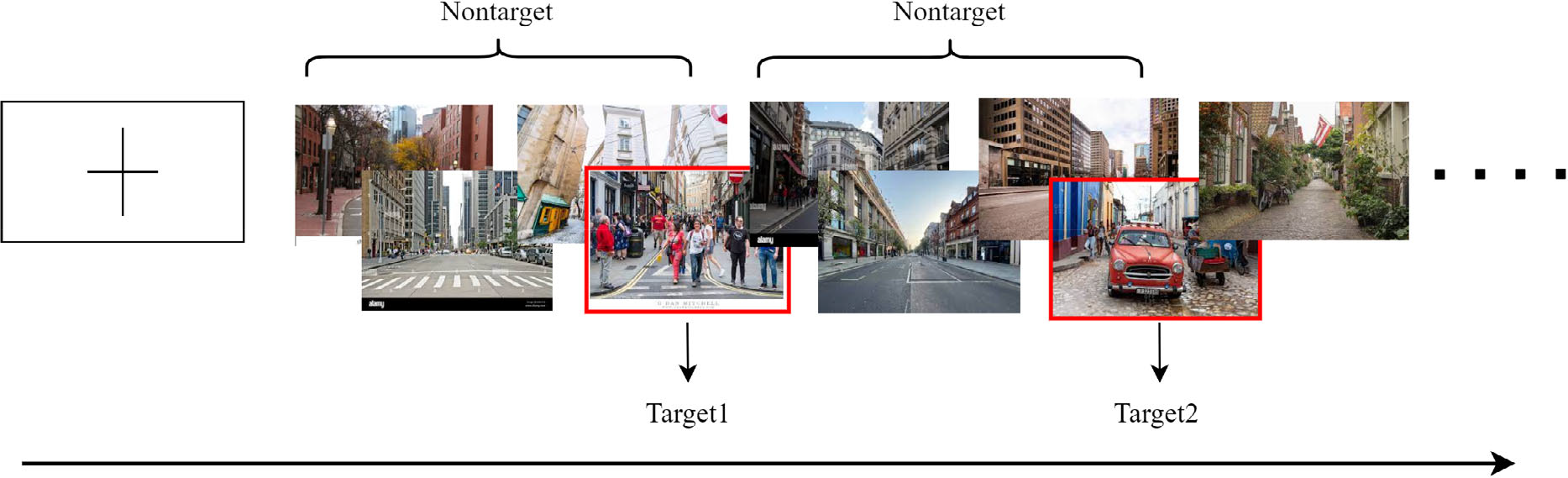
Rapid serial visual presentation (RSVP) paradigm of BCI competition.

Each subject’s EEG signals were collected in blocks with a prompt in the center of the screen before each block started. The image sequence was presented in trials. Each trial started with a cross-prompting the subject to focus on the center of the screen, and each trial contained 50 images, of which the target type and number were not fixed (up to five target images), and each image was presented in the center of the screen at a rate of 10 images per second, with each block containing 10 trials. The flow of the experiment is displayed in Fig. 2.

Fig. 2

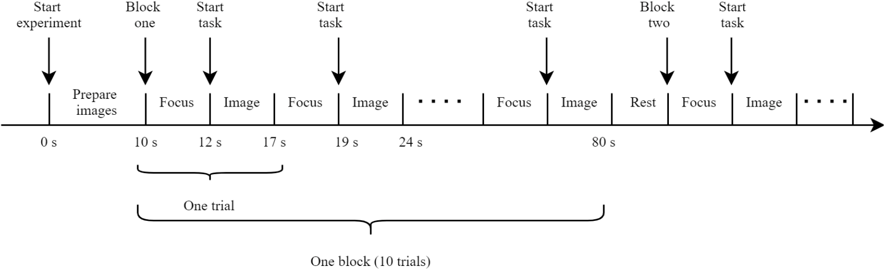
Experimental procedure.

2.2 Data collection

Experimental data were collected using Neuracle 64-channel EEG acquisition equipment. The last four channels were not EEG channels; instead, they were ECG, HEOR, HEOL, VEOU, and VEOL. The original sampling rate was 1000 Hz, and the data were sampled down to 250 Hz. The organizer prepared EEG data of 24 subjects for competition teams to use for training. In the final BCI competition, six healthy students were assigned to a real-time assessment.

2.3 Evaluation metric

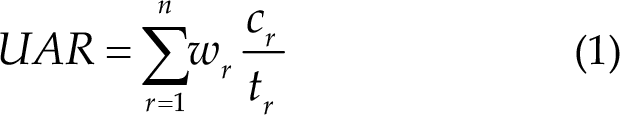
In the competition, unweighted average recall (UAR) [24] was used as the scoring criterion, where n denotes the total number of categories, w_r denotes the weight factor applied for each category, which is set to [0.33, 0.33, 0.33], t_r denotes the number of images per category, and c_r was the number of correct predictions per category. In particular, the system calculated the UAR for each trial and finally averaged all blocks for scoring.

U A R = \sum_{r = 1}^{n} w_{r} \frac{c_{r}}{t_{r}}

2.4 Deep learning training techniques

The same model performs differently to various training approaches. Using appropriate training techniques is critical. Here, we list four robust training methods to help models converge to superior generalization.

2.4.1 Mixup

Mixup is an effective technique for training deep learning models that combine elements from two training examples to create a novel synthetic example [25]. This technique is used for improving the robustness of the model by encouraging the model to learn a smooth decision boundary between various classes. In Mixup, two training examples, x ₁ and x ₂, are considered and a novel sample, x _mix, is created by interpolating the values of input features, and corresponding labels, y ₁ and y ₂. This new sample x _mix and label y _mix are then used instead of the original sample and label during training. Interpolation weight λ is typically sampled from a Beta distribution, that is, Beta(α, α), where α is a hyperparameter, and α should be greater than zero. The formula for Mixup is as follows:

x_{mix} = λ x_{1} + (1 - λ) x_{2}

y_{mix} = λ y_{1} + (1 - λ) y_{2}

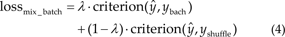
In practice, Mixup loss is typically calculated in batches. First, a batch of data x _batch and corresponding labels y _batch are randomly disrupted, and the disrupted data and corresponding labels are recorded as x _shuffle and y _shuffle, respectively. The input to the deep learning model is x _{batch_mix}, which is computed using Eq. (2), and the predicted output is $\hat{y}$ . The Mixup loss is divided into two parts as shown in Eq. (4). The criterion is the conventional optimization loss function. The left part calculates the loss of y _batch and $\hat{y}$ and multiplies λ; the right part calculates the loss of y _shuffle and $\hat{y}$ and multiplies (1 – λ). The sum of the two parts is the Mixup loss.

\begin{matrix} {loss}_{mix _batch} = λ \cdot criterion (\hat{y}, y_{bach}) \\ + (1 - λ) \cdot criterion (\hat{y}, y_{shuffle}) \end{matrix}

when Mixup is applied appropriately and hyperparameter α is set to a small size, then it should not alter the underlying distribution of EEG data. However, when the hyperparameter α is extremely large, then it could generate data points that differ considerably from the original data and change the underlying distribution. The optimal value of α may vary depending on the specific problem and the architecture of the model. Several studies [26 –28] have revealed that Mixup could improve performance in terms of out-of-distribution EEG data and generalization of deep learning models.

2.4.2 Stochastic weight averaging

Stochastic weight averaging (SWA) is a regularization technique that is used in deep learning to improve the generalization of neural networks [29]. SWA involves averaging the weights of multiple models obtained during training to produce a single set of weights. This average set of weights tends to be smoother and more robust than individual models, which reduces overfitting and improves the ability of the model to generalize to new data. The method is stochastic because weight updates are performed using the minibatches of randomly sampled data, which lead to random fluctuations in the weights. The averaging process reduces these fluctuations and stabilizes the final set of weights, which improves performance on unseen data. SWA is simple to implement, computationally efficient, and can be combined with other regularization techniques for improvement.

2.4.3 Label smoothing

Label smoothing is used in deep learning to prevent overfitting and improve generalization [30]. By adjusting the labels of the training data to be less certain, the model becomes robust and less likely to overfit the training set. The model replaces the one-hot encoded labels with a softer version, where the target class has a high probability, and the other classes have small probability. This phenomenon discourages the model from becoming too confident in its predictions, which reduces overfitting and encourages the exploration of the output space.

y^{LS} = y (1 - θ) + \frac{θ}{K}

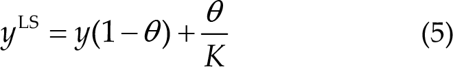
where y is the one-hot encoded target label, y ^LS is the smoothed label, θ is the smoothing factor, and K is the number of classes. The smoothing factor θ controls the degree of label smoothing. A common value for θ is 0.1.

2.4.4 Focal loss

Focal loss is a loss function designed for training deep learning models to address class imbalance in datasets [31]. The imbalance occurs when the number of samples of one class is considerably larger than the other class, which leads to the model being biased toward the majority class. Focal loss modifies the standard cross-entropy loss by down-weighting the loss for well-classified examples and increasing the loss for misclassified examples. The focus on hard samples improves model performance in the cases of imbalanced datasets. The focal loss has a modulating factor (focusing parameter, γ) ranging from zero to infinity, which determines the rate at which easy examples are down-weighted.

FL (p_{t}) = - {(1 - p_{t})}^{γ} \log p_{t}

2.5 Descriptions of algorithms

The algorithms of the top 5 winning teams in the final round, with team names Brainstorming, NaoDianXinHaoYaoFenDui, BLC&HI, Ecust_BCILab, and UMBCI, were presented. For simplicity, these teams were labeled with numbers, that is, Teams 1, 2, 3, 4, and 5, respectively.

2.5.1 Algorithm of Team 1

The algorithm architecture of Team 1 is displayed in Fig. 3. We selected the first 59 EEG channels with a segmentation time window of 1 s (that is, 250 time sample points). Next, we preprocessed the segmented data, that is (a) detrending, (b) applying 12th-order 30 Hz Chebyshev low-pass filter with zero phase, and (c) using z-score normalization. Next, three models, namely DeepConvNet, EEGNet, and EEGNet, were trained on a large training dataset with training tricks, that is, Mixup, SWA procedure, and focal loss. The maximum number of training epochs was set to 200, and the early stop strategy was adopted to prevent overfitting, with its patience set to 50. We turned on the SWA strategy when each model was trained for approximately 150 epochs. We used a grid search algorithm to determine the best hyperparameters for each model on the validation set, that is, a search range from 0.2 to 0.4 for hyperparameter α of Mixup and a search range from 0 to 2 for the hyperparameter γ of focal loss. Next, we applied the Monte Carlo method [32] to obtain the best weighting ensemble weights for models trained on the validation dataset as displayed in the algorithm of Team 1. The ratio of training and validation sets was 4:1. Next, for each trial of 50 images, we applied ensemble models to obtain weighted integration probability and subsequently used long short-term memory (LSTM) [33] to perform the sequence labeling to extract sequence information in trials, as displayed in Fig. 4. Finally, the weighted integration probability and the LSTM calibrated probability were added to obtain the final output.

Fig. 3

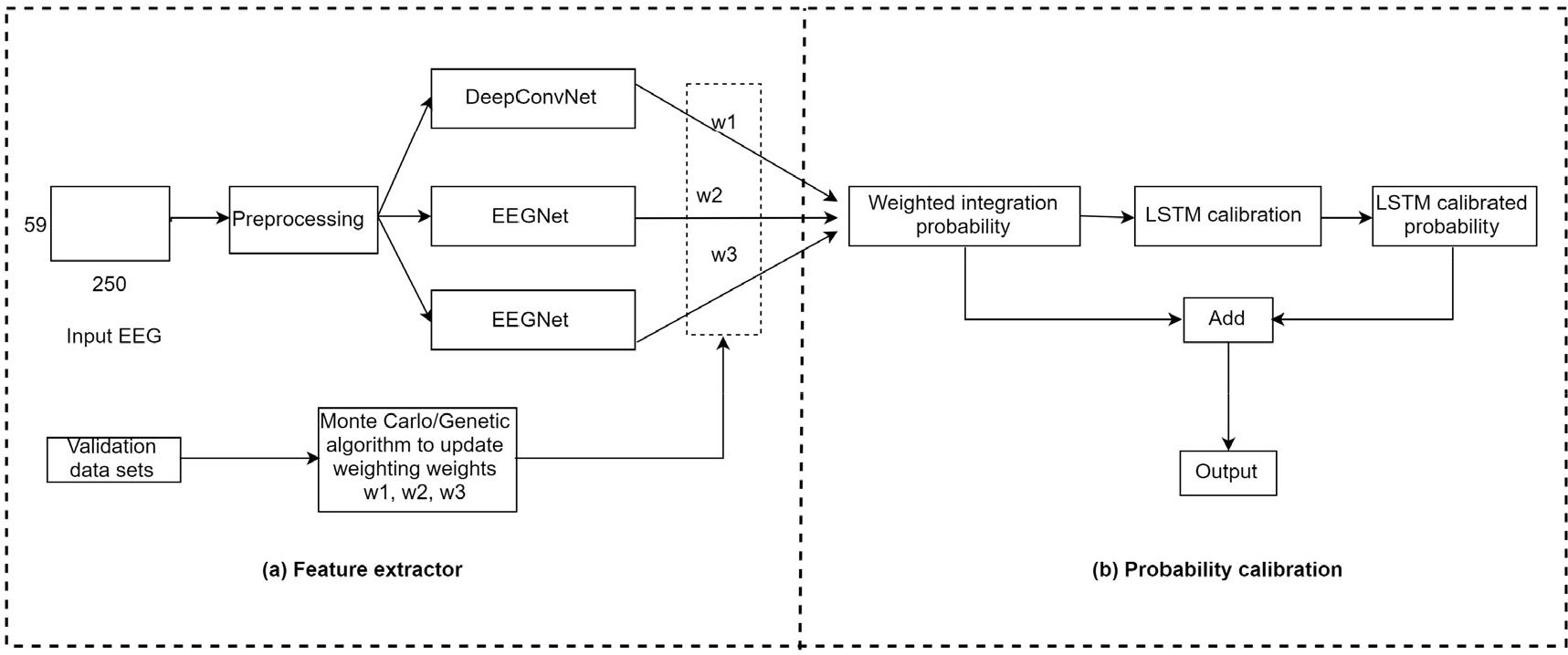
Algorithm description of Team 1. The model consists of (a) a feature extractor and (b) probability calibration.

Fig. 4

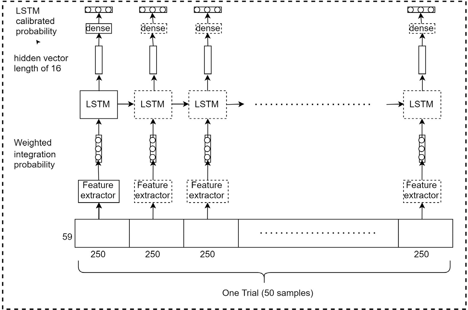
Description of the LSTM calibration block in part (b) of Team 1’s algorithm (Fig.3).

2.5.2 Algorithm of Team 2

The description of the algorithm for Team 2 is displayed in Fig. 5. The algorithm consists of two parts, namely (a) a single model and (b) ensemble models. The single model has two branches from the input. One branch goes through four convolutional layers (DeepConvNet) whose inputs are the first 59 EEG channels, whereas the other branch has only one convolutional layer whose inputs are five channels, namely ECG, HEOR, HEOL, VEOU, and VEOL. The filter sizes of the max pooling layers were set to (1, 2), and the dropout values were set to 0.3. The features obtained from both branches were then concatenated after Flatten and LayerNorm operations. The first fully connected layer has two output neurons of which the value of the second neuron is copied to the new third neuron. The second fully connected layer has three output neurons. Finally, the new output of the first fully connected layer is multiplied by the output of the second fully connected layer to obtain the output probability of the single model.

Fig. 5

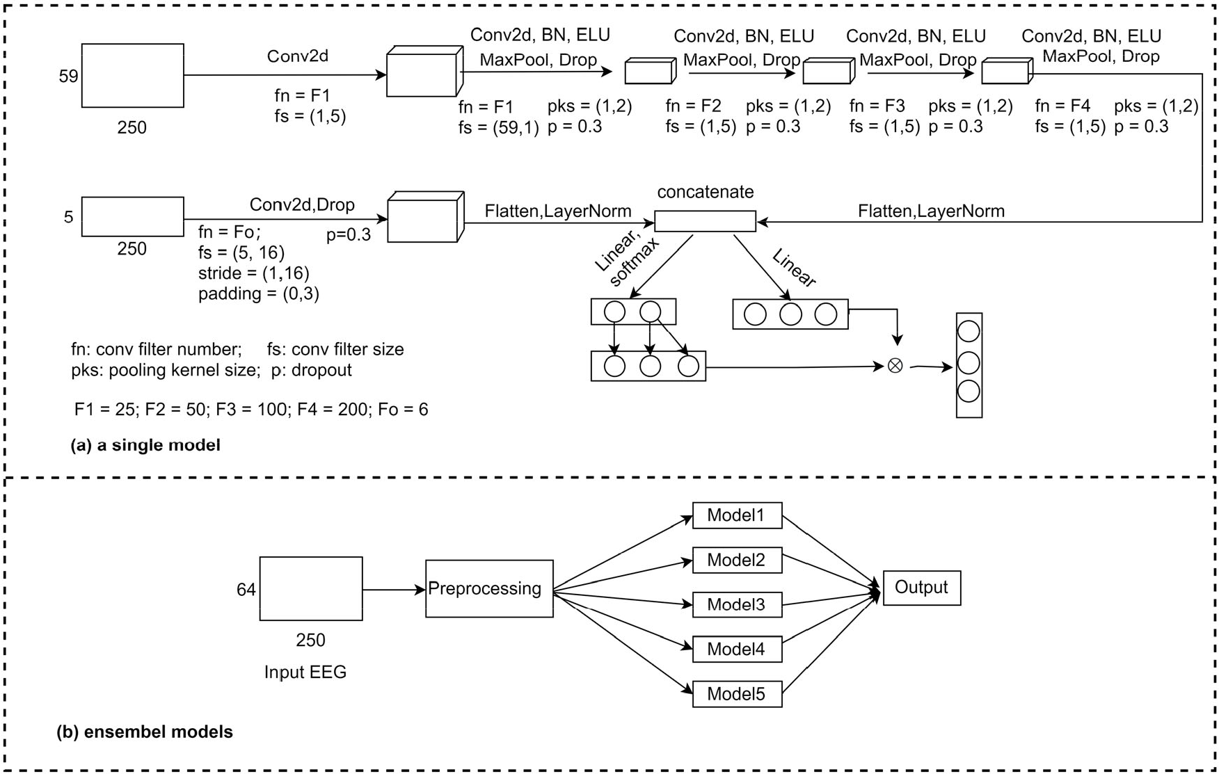
Algorithm description of Team 2. It consists of (a) single model and (b) ensemble models.

Algorithm 1:

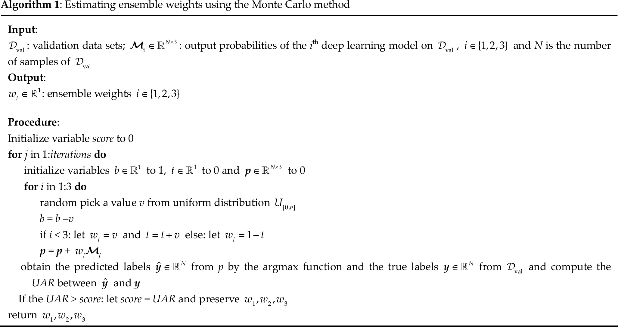
Estimating ensemble weights using the Monte Carlo method

The ensemble model is the algorithm of Team 2, which selected the first 64 channels with a segmentation time window of 1 s (i.e., 250 time sample points), and subsequently filtered them with a third-order 0.5 to 15 Hz butter bandpass with zero phase and normalized with the z-score. These preprocessed data were then inputted into five single models to obtain the final output. All five models with the same structure and 187,357 training parameters were trained on five downsampled versions of the original dataset. Each model was trained on a distinct subset of the data, which allowed the models to learn different representations of the data. This measure can improve the classification performance of the model.

2.5.3 Algorithm of Team 3

The algorithm of Team 3 is detailed in Fig. 6. In this approach, the first 59 EEG channels were selected, and the data were segmented into 1 s windows (equivalent to 250 time sample points). The data were then preprocessed using max–min normalization before being inputted into the EEGNet model for the final output. This approach emphasized the importance of careful EEG data selection to achieve optimal performance in BCI applications, which is explained in Section 4.1.3.

Fig. 6

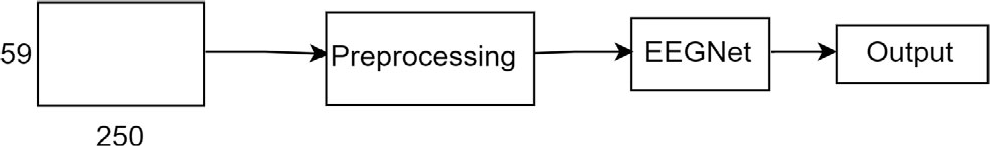
Algorithm description of Team 3.

2.5.4 Algorithm of Team 4

Team 4 selected 57 channels from the first 59 EEG channels (channels C6 and T7 were excluded) and set the segmentation time window to 256. Next, they re-referenced using the average of channels C6 and T7 and applied a 50 Hz notch filter and a third-order 0.5–30 Hz butter bandpass filter and normalized using the z-score. Finally, they adopted EEG-Inception to obtain the final output. The algorithm for Team 4 is shown in Fig. 7.

Fig. 7

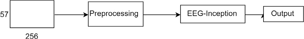
Algorithm description of Team 4.

2.5.5 Algorithm of Team 5

The algorithm for Team 5 is displayed in Fig. 8, which consists of parts (a), (b), and (c). In part (a), they selected the first 59 EEG channels with a segmentation time window of 1.5 s (375 time sample points). Next, they applied 50, 20, 10, 30, and 40 Hz notch filters on the data, followed by debaseline drift, and followed by an eighth-order butter bandpass filter from 1 to 90 Hz. 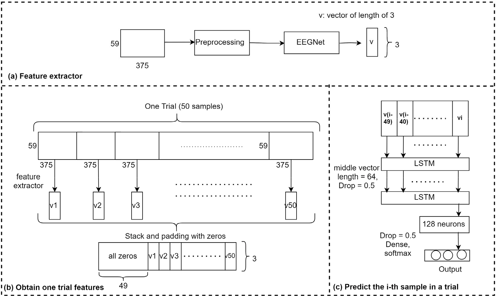The preprocessed data were inputted into EEGNet to obtain an embedded vector v of length 3. In part (b), Team 5 obtained 50 embedded vectors from 50 EEG samples in a trial; the vectors were then stacked and padded with zeros. In part (c), Team 5 adopted stacked LSTMs to predict the i ^th sample in a trial with previous 49 vectors and its vector information to obtain the final output. They adopted a single EEGNet model to convert the raw EEG data to embedded vectors and subsequently used stacked LSTMs to predict the labels of each EEG data sample in a trial, which reveals that the information from previous samples is considered when predicting the i ^th sample.

Fig. 8

Algorithm of Team 5. It consists of (a) a feature extractor, (b) obtaining one trial features and (c) predicting the ith sample in a trial.

3 Results

The results are displayed in Fig. 9. Unweighted average recall was the official evaluation method, and the recall for each category (nontarget, person, and car) was presented. Among samples with category nontarget, Team 1 achieved the highest correct identification rate of 0.7538, followed by Team 4 with 0.7335, Team 3 with 0.7122, and finally Teams 2 and 5 with 0.6463 and 0.6286, respectively. In samples with category persons, the teams with the highest to lowest correct identification rates were Teams 5, 2, 3, 1, and 4 with 0.4089, 0.3816, 0.3641, 0.3485, and 0.3429, respectively. In samples with category car, the teams with high to low correct recognition rates were Teams 2, 1, 3, 4, and 5 with 0.5754, 0.5407, 0.4939, 0.4896, and 0.4648, respectively. On the official UAR rating criteria, the scores for Teams 1 to 5 were 0.5477, 0.5344, 0.5234, 0.5220, and 0.5008, respectively.

Fig. 9

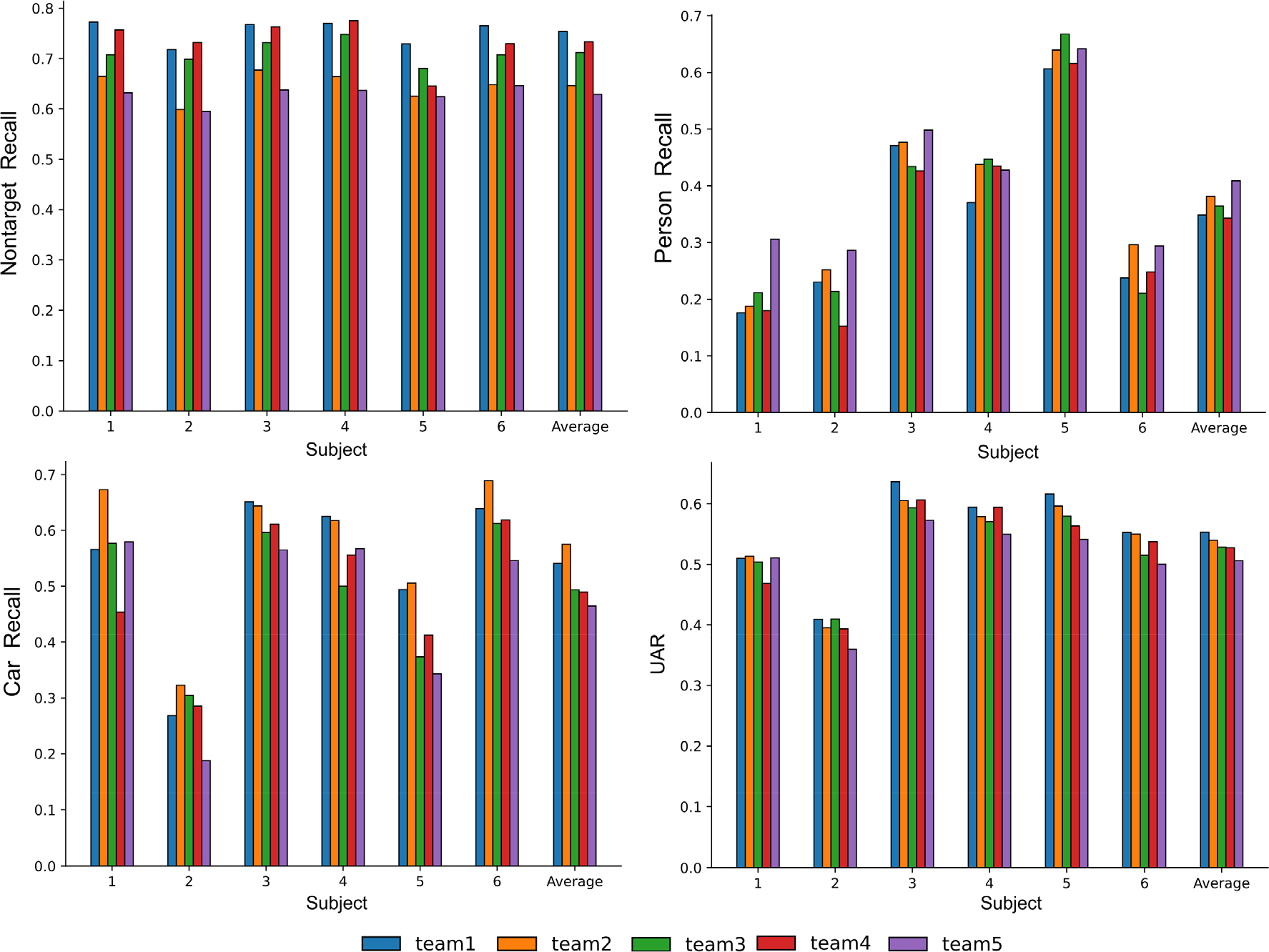
Recall and UAR comparisons of all teams

4 Discussion

4.1.1 Analysis of results

The top five teams in the competition used deep learning models and achieved similar satisfactory results. The top two teams used ensemble models, and Teams 3 and 4 used a single model, which indicated that better results can be obtained with a proper model ensemble strategy. Team 5 also used ensemble models but did not achieve satisfactory results, and a possible reason could be the large variance of the ensemble models. Furthermore, the stacked LSTMs of Team 5 overfitted the sequence information of each trial of the training data, which resulted in the inability to generalize effectively on new subjects. Fig. 9 reveals that for samples of category nontarget, the models of Teams 1, 3, and 4 achieve higher recognition rates than the models of Teams 2 and 5 do, which indicates that the models of these three teams have more preference for nontarget samples in category weights during training. Adjusting the loss weights between nontarget and targets to achieve higher UAR is difficult.

4.1.2 Analysis of feature maps

We visualized the EEG data of the final six subjects (after the preprocessing step of Team 1), as displayed in part (a) of Fig. 10. The heat maps in the left half of (a) represent the average of the EEG signals of these six subjects, where the horizontal coordinate represents the time in seconds, and the vertical coordinate represents the index of the electrodes. From top to bottom, these images correspond to nontarget, person, and car, respectively. From part (a) of Fig. 10, the nontarget sample differs considerably from the two target samples. However, observing the difference between the person and car samples is difficult.

Fig. 10
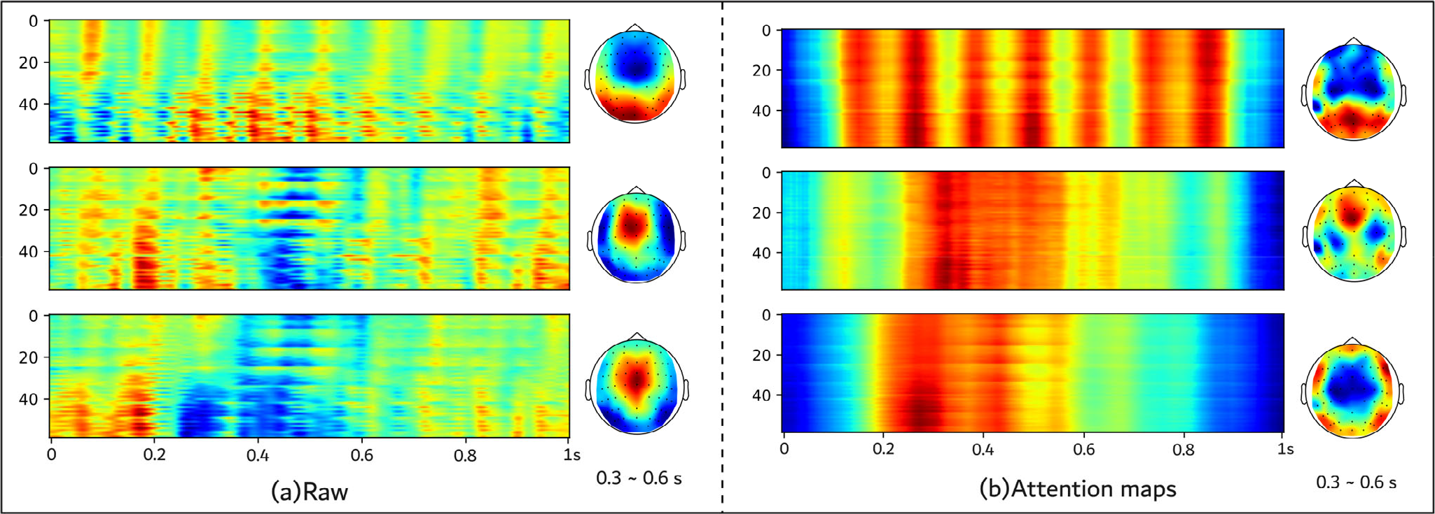
Visualization of (a) the averaged EEG signal and its topography (0.3–0.6 s) and (b) attention map and its topography(0.3–0.6 s). From top to bottom, these images correspond to nontarget, person, and car, respectively.

Therefore, we selected the top 15 channels of the target samples distributed with higher energy in the head (AF3, C1, C2, C3, CP1, Cz, F1, F2, F3, FC1, FC2, FC3, FCz, Fp1, Fz, and Pz) and performed time–frequency analysis for each category and averaged the time–frequency heat maps of the 15 channels (Fig. 11). We could determine a distinct energy region at 0.2 to 0.3 s in the low-frequency band for evoked potentials triggered by the car sample, and such an energy region was not observed for evoked potentials triggered by the person sample. How well the models capture such temporal variation is crucial for distinguishing the person sample from the car sample.

Fig. 11
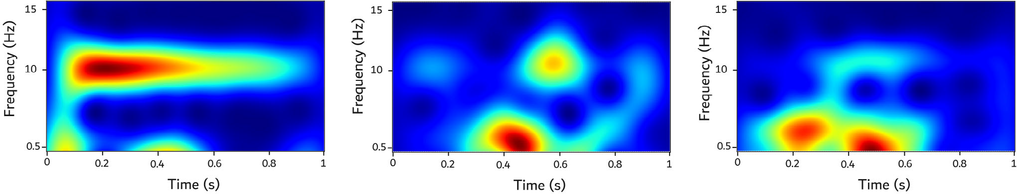
Time–frequency analysis heat maps corresponding to nontarget, person, and car from left to right.

To understand the spatial and temporal locations captured by our model on the EEG data of these six new subjects, we visualized the attention maps of all convolutional layers in the feature extractors (DeepConvNet and two EEGNet) of Team 1 using Grad-CAM [34] (with “aug_smooth” parameter set to true, which rendered the CAM better centered around objects.) as an example, and the results are displayed in (b) in Fig. 10. The attention heat maps reveal that for samples with category nontarget, the model can provide a distinct frequency feature. For the samples in person category and samples in the car category, the model focused on the region from 0.28 to 0.55 s, and the region from 0.2 to 0.48 s, respectively. A significant temporal shift was observed between the attention maps of the two targets, which could imply that the model considers the temporal difference. These findings indicate that our model can capture the temporal location features of the target category. The EEG topography reveals that on the samples of category nontarget, the spatial location of the model’s attention matches the spatial location of the original EEG signals, and on the samples of category person, the spatial location of the model attention map is concentrated in regions FCz, FC1, F1, and Fz, whereas the original spatial location was concentrated in FCz, FC1, F1, and Cz. On the samples of the category car, our model attended to the opposite spatial distribution to the original spatial distribution. These findings indicated that our model can capture spatial features across nontarget samples but is weak in capturing spatial features across target samples of subjects. This phenomenon could be attributed to the difference in the size, shape, cranial density, and hair of the heads of subjects resulting in various spatial distributions, which renders capturing distinct P300 features difficult. Improving the model to capture the spatial features of the target sample across subjects is challenging.

4.1.3 Analysis of data selection

The number of training parameters for the algorithm of each team is as follows: Team 1: 439,147; Team 2: 936,785; Team 3: 2,384; Team 4: 25,673; and Team 5: 130,422. The algorithm of Team 3 achieved not only excellent UAR performance but also low complexity, which could be attributed to the removal of bad data samples. However, Team 3 did not provide the training code for their algorithm, rendering replicating their approach difficult. Therefore, we analyzed the raw EEG data of 24 individuals after detrending and 30 Hz low-pass filtering. We observed that not all subjects achieved excellent EEG quality. Subjects 6, 9, 13, and 18 exhibited poor data quality because of the presence of bad channels in the raw signal. The recorded signals of other subjects were not affected by the poor channel data. To illustrate this phenomenon, we selected Subject 2, with superior EEG quality, and Subject 6, with inferior EEG quality, as representatives and plotted their corresponding EEG signals after averaging the EEG signals of each category (Fig. 12). Because of computational resource limitations, we could not test the hypothesis that performance improved when corrupted data were removed from the original dataset. However, Ghorbani et al. confirmed this result [35]. Further research is necessary to investigate the effect of data quality on algorithm performance and determine the optimal approach for handling bad data samples in EEG classification tasks.

Fig. 12
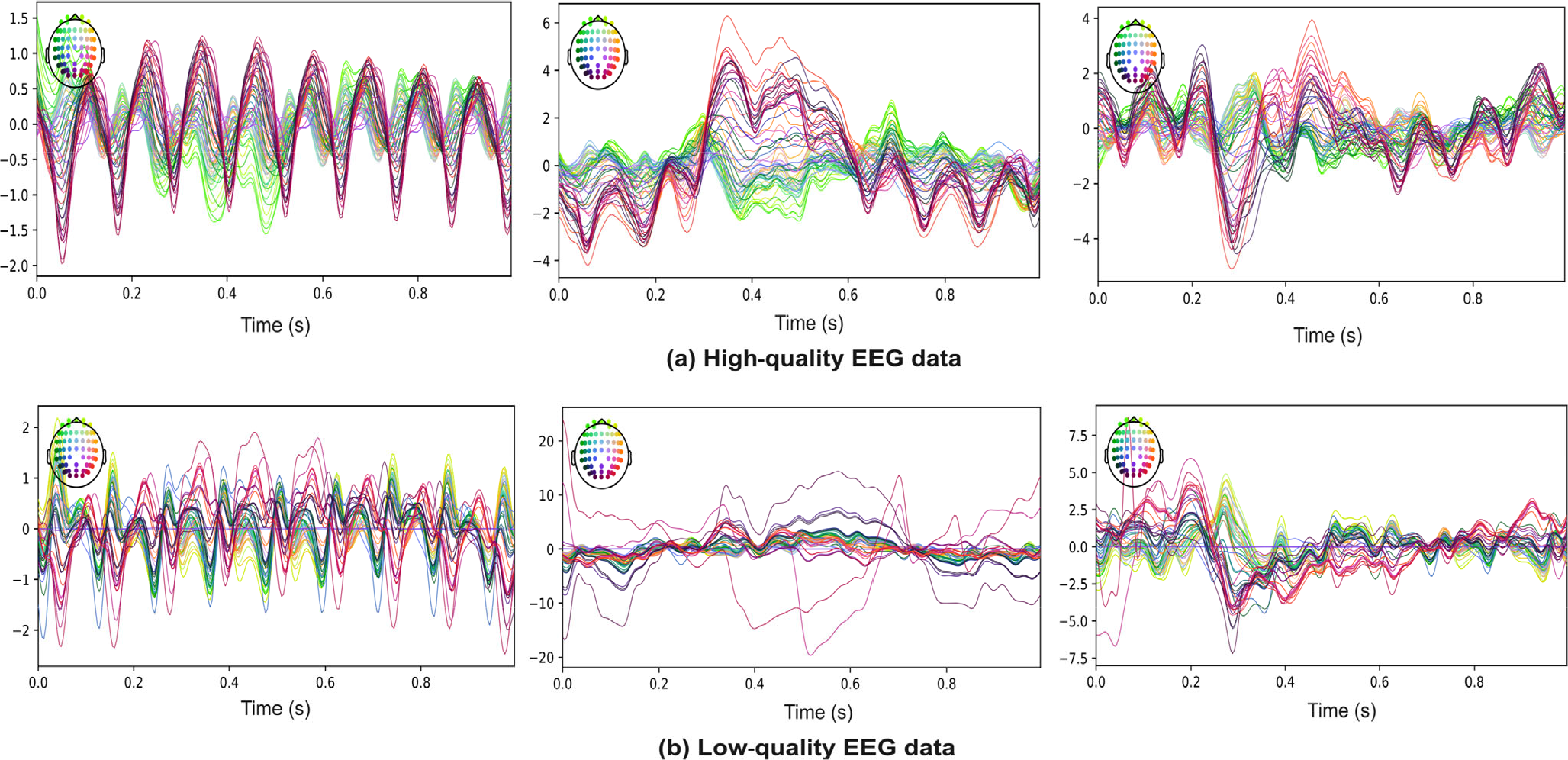
Average EEG signals for each category. The diagrams from left to right correspond to the categories nontarget, person, and car, respectively. Here, (a) and (b) represent the averaged EEG signals of subjects 2 and 6, respectively.

5 Conclusion

This study provided a detailed analysis of the algorithms of the top five teams for RSVP detection and detailed their performance on the final dataset. The results demonstrated that incorporating reasonable deep learning training methods and ensemble models could improve the stability and generalization performance of the trained models. Deep learning methods were successfully applied to EEG signals, and future research should explore the potential of these methods. We plan to investigate larger scale EEG models to improve generalization performance for downstream tasks. The findings contribute to the research on the use of deep learning in EEG analysis.

Footnotes

Ethical approval

This work was approved by the Institutional Review Board of Tsinghua University.

Conflict of interests

All contributing authors have no conflict of interests.

Funding

This work is granted by the Special Projects in Key Fields Supported by the Technology Development Project of Guangdong Province (Grant No. 2020ZDZX3018), the Special Fund for Science and Technology of Guangdong Province (Grant No. 2020182), the Wuyi University and Hong Kong & Macao joint Research Project (Grant No. 2019WGALH16).

Authors’ contribution

Zehui Wang: Software, writing the original draft. Hongfei Zhang: Software, writing the original draft. Zhouyu Ji: Software. Yuliang Yang: Software. Hongtao Wang: Conceptualization, validation. All the authors approved the final manuscript.

References

Rebsamen

Guan

Zhang

, et al. A brain controlled wheelchair to navigate in familiar environments. IEEE Trans Neural Syst Rehabil Eng 2010, 18(6): 590–598.

Liang

Zhao

, et al. Design of assistive wheelchair system directly steered by human thoughts. Int J Neural Syst 2013, 23(3): 1350013.

Polich

. Updating P300: an integrative theory of P3a and P3b. Clin Neurophysiol 2007, 118(10): 2128–2148.

Picton

. The P300 wave of the human event-related potential. J Clin Neurophysiol 1992, 9(4): 456–479.

Farwell

Donchin

. Talking off the top of your head: toward a mental prosthesis utilizing event-related brain potentials. Electroencephalogr Clin Neurophysiol 1988, 70(6): 510–523.

Wang

Huang

, et al. An event related potential electroencephalogram signal analysis method based on denoising auto-encoder neural network (in Chinese). Contr Theory Appl 2019, 36(4): 589–595.

Liu

, et al. Deep learning based on Batch Normalization for P300 signal detection. Neurocomputing 2018, 275: 288–297.

Wang

Chen

, et al. ST-CapsNet: linking spatial and temporal attention with capsule network for P300 detection improvement. IEEE Trans Neural Syst Rehabil Eng 2023 , PP, doi 10.1109/TNSRE.2023.3237319.

Kundu

Ari

. MsCNN: a deep learning framework for P300-based brain–computer interface speller. IEEE Trans Med Robot Bionics 2020, 2(1): 86–93.

10.

Hajinoroozi

Mao

Lin

, et al. Deep transfer learning for cross-subject and cross-experiment prediction of image rapid serial visual presentation events from EEG data. In Augmented Cognition. Neurocognition and Machine Learning. AC 2017. Lecture Notes in Computer Science, vol 10284 Schmorrow

Fidopiastis

, Eds. Cham: Springer, 2017, pp 45–55.

11.

Lees

Dayan

Cecotti

, et al. A review of rapid serial visual presentation-based brain-computer interfaces. J Neural Eng 2018, 15(2): 021001.

12.

Subasi

Ismail Gursoy

. EEG signal classification using PCA, ICA, LDA and support vector machines. Expert Syst Appl 2010, 37(12): 8659–8666.

13.

Mika

Ratsch

Weston

, et al. Fisher discriminant analysis with kernels. In Neural Networks for Signal Processing IX: Proceedings of the 1999 IEEE Signal Processing Society Workshop (Cat. No.98TH8468) . Madison, WI, USA, 2002, pp 41–48.

14.

Gerson

Parra

Sajda

. Cortically coupled computer vision for rapid image search. IEEE Trans Neural Syst Rehabil Eng 2006, 14(2): 174–179.

15.

Fuhrmann Alpert

Manor

Spanier

, et al. Spatiotemporal representations of rapid visual target detection: a single-trial EEG classification algorithm. IEEE Trans Biomed Eng 2014, 61(8): 2290–2303.

16.

Lawhern

Solon

Waytowich

, et al. EEGNet: a compact convolutional neural network for EEG-based brain–computer interfaces. J Neural Eng 2018, 15(5): 056013.

17.

Schirrmeister

Springenberg

Fiederer

LDJ

, et al. Deep learning with convolutional neural networks for EEG decoding and visualization. Hum Brain Mapp 2017, 38(11): 5391–5420.

18.

Santamaria-Vazquez

Martinez-Cagigal

Vaquerizo-Villar

, et al. EEG-inception: a novel deep convolutional neural network for assistive ERP-based brain-computer interfaces. IEEE Trans Neural Syst Rehabil Eng 2020, 28(12): 2773–2782.

19.

Wang

Pei

, et al. Performance enhancement of P300 detection by multiscale-CNN. IEEE Trans Instrum Meas 2021, 70: 1–12.

20.

. Transfer learning for brain-computer interfaces: a euclidean space data alignment approach. IEEE Trans Biomed Eng 2020, 67(2): 399–410.

21.

Rivet

Souloumiac

, Attina V, et al. xDAWN algorithm to enhance evoked potentials: application to brain-computer interface. IEEE Trans Biomed Eng 2009, 56(8): 2035–2043.

22.

. Review of training-free event-related potential classification approaches in the World Robot Contest 2021. Brain Science Advances 2022, 8(2): 82–98.

23.

Zhang

Wang

, et al. An improved EEGNet for single-trial EEG classification in rapid serial visual presentation task. Brain Science Advances 2022, 8(2): 111–126.

24.

, et al. Decoupling representation learning for imbalanced electroencephalography classification in rapid serial visual presentation task. J Neural Eng 2022, 19(3): 10.1088/1741–10.1088/2552/ac6a7d.

25.

Zhang

Cisse

Dauphin

, et al. Mixup: beyond empirical risk minimization. arXiv 2017, arXiv: 1710.09412. https://arxiv.org/abs/1710.09412

26.

Kostas

Rudzicz

. Thinker invariance: enabling deep neural networks for BCI across more people. J Neural Eng 2020, 17(5): 056008.

27.

Han

Jeong

. Domain generalization for session-independent brain–computer interface. In 2021 9th International Winter Conference on Brain–Computer Interface (BCI). Gangwon, Korea (South), 2021, pp 1–5.

28.

Lei

Belkacem

Wang

, et al. A convolutional neural network-based diagnostic method using resting-state electroencephalograph signals for major depressive and bipolar disorders. Biomed Signal Process Contr 2022, 72: 103370.

29.

Izmailov

Podoprikhin

Garipov

, et al. Averaging weights leads to wider optima and better generalization. arXiv 2018, arXiv: 1803.05407. https://arxiv.org/abs/1803.05407

30.

Müller

Kornblith

Hinton

. When does label smoothing help? In 33rd Conference on Neural Information Processing Systems (NeurIPS 2019). Vancouver, Canada, 2019.

31.

Lin

Goyal

Girshick

, et al. Focal loss for dense object detection. IEEE Trans Pattern Anal Mach Intell 2020, 42(2): 318–327.

32.

James

. Monte Carlo theory and practice. Rep Prog Phys 1980, 43(9): 1145–1189.

33.

, et al. A review of recurrent neural networks: LSTM cells and network architectures. Neural Comput 2019, 31(7): 1235–1270.

34.

Selvaraju

Cogswell

Das

, et al. Grad-CAM: visual explanations from deep networks via gradient-based localization. In 2017 IEEE International Conference on Computer Vision (ICCV) . Venice, Italy, 2017, pp 618–626.

35.

Ghorbani

, Zou J. Data shapley: equitable valuation of data for machine learning. arXiv 2019, arXiv: 1904.02868. https://arxiv.org/abs/1904.02868

A review of deep learning methods for cross-subject rapid serial visual presentation detection in World Robot Contest 2022

Abstract

Keywords

1 Introduction

2 Methods

2.1 Experimental paradigm

2.2 Data collection

2.3 Evaluation metric

2.4 Deep learning training techniques

2.4.1 Mixup

2.4.2 Stochastic weight averaging

2.4.3 Label smoothing

2.4.4 Focal loss

2.5 Descriptions of algorithms

2.5.1 Algorithm of Team 1

2.5.2 Algorithm of Team 2

2.5.3 Algorithm of Team 3

2.5.4 Algorithm of Team 4

2.5.5 Algorithm of Team 5

3 Results

4 Discussion

4.1.1 Analysis of results

4.1.2 Analysis of feature maps

4.1.3 Analysis of data selection

5 Conclusion

Footnotes

Ethical approval

Conflict of interests

Funding

Authors’ contribution

References